Article

A Comparative Design of a Campus Microgrid Considering a Multi-Scenario and Multi-Objective Approach

1
Department of Electrical and Electronics Engineering, University of the Ryukyus, Okinawa 903-0213, Japan
2
Department of Electrical and Electronics Engineering, University of Fukui, 3-9-1 Bunkyo, Fukui 910-8507, Japan
3
Electrical Engineering Department, Faculty of Energy Engineering, Aswan University, Aswan 81528, Egypt
4
Financial University under the Government of the Russian Federation, 124167 Moscow, Russia
*
Authors to whom correspondence should be addressed.
Submission received: 19 April 2021 / Revised: 17 May 2021 / Accepted: 18 May 2021 / Published: 21 May 2021
(This article belongs to the Special Issue State-of-the-Art Energy Related Technologies in Japan 2021)

Abstract

:
This article proposes a plan to replace real-time power with constant power from the grid to reduce costs and reduce the impact of the micro-grid on the main grid at the same time. Most of the peak electricity consumption periods of universities or some enterprise institutions are during the daytime. If solar energy can be used reasonably at this time, it can provide a good guarantee of peak power. In this study, a grid-linked solar-plus-storage micro-grid was used to supply power to a university located in Okinawa, Japan. The non-dominated sorting genetic algorithm II (NSGA-II) was used to optimize the model size, and the loss of power supply probability (LPSP), life cycle cost (LCC), and waste of energy (WE) were taken as the optimization indicators. For this study, three scenarios were considered where the first scheme (Case 1) was a comparison scheme, which used a PV battery and real-time power from the infinity bus. Both the second and third cases used constant power. While Case 2 used constant power throughout the year, Case 3 used daily constant power. The optimal solutions for the power supply units were grouped into three cases where Case 1 was found to be the most expensive one. It was found that the costs of Cases 2 and 3 were 62.8% and 63.3% less than Case 1. As a result, the waste of energy was found to be more significant than Case 1: 70 times and 60 times, respectively. On the contrary, Case 1 had 15.2% and 16.7% less carbon emissions than Case 2 and Case 3, respectively. This article put forward the idea of constant power supply growth at the financial markets, which breaks the traditional way in which the power supply side follows the user’s consumption. While reducing costs, it reduces the impact on large-scale power grids and can also ensure the reliability of campus microgrids.

1. Introduction and Background

As the primary renewable energy sources, wind and solar energy systems already have a high level of development and utilization. The sustainability of these hybrid renewable energy or alternative energy power generation systems is very important [1]. In addition, the flexibility in the power system is mainly undertaken by the energy storage system [2]. At the same time, renewable-based microgrids have seen enormous interest and are being adopted for numerous infrastructures, which increases the power reliability along with the main grid [3,4].
The photovoltaic (PV) cell technologies, energy conversion efficiency, economic analysis, energy policies, environmental impact, various applications, prospects, and progress were comprehensively reviewed and presented by Hosenuzzaman et al. [5]. It was found that PV is an easy way to capture solar energy, and as such, PV-based power generation has also rapidly increased in the power system. However, since this mass introduction of the PV system is carried out by considering sufficient system stability, energy storages are indispensable for system stability. For example, they integrate renewable energy, adjust peaks, enhance grid resilience, and support energy self-sufficiency [6,7]. Energy storage systems’ (ESS) operation plays an essential role in transitioning the renewable energy system into a sustainable power system.
Barbour et al. [8] illustrated that community energy storage has a number of advantages over household storage, including decreasing the total amount of storage deployed, decreasing surplus PV generation, which must be exported to the wider network, and subsequently, increasing the self-sufficiency of local smart energy communities. There is reason to believe that a larger community energy storage system will be better than many independent small energy storage systems. There are many articles that have designed storage/grid systems. The campus microgrid proposed by Bracco et al. [9] involved an energy management scheme that minimized the cost while meeting the electrical and thermal constraints. However, they did not mention the loss of power supply probability (LPSP) and waste of energy (WE). Mohammad Masih Sediqi et al. [10] considered two objectives, which were the minimization of the life cycle cost (LCC) and the maximization of system LPSP. They used the genetic algorithm (GA) to find the optimal values of the total area occupied by the PV array, the total swept area by the wind turbines, and the number of batteries [10]. However, the article did not mention how to deal with wasted power. The use of renewable energy inevitably results in the lossof some wind power or some solar power. Moreover, this wasted energyis difficult to reuse because it is difficult to predict, and the amount that can be used is less and unevenly distributed. In this article, the wastedenergy was intensive, which could be easier to use.
Zhijia et al. [11] compared four typical hybrid energy systems (HESs), i.e., photovoltaic and wind turbine, photovoltaic and diesel generator, wind turbine and diesel generator, and photovoltaic, wind turbine, and diesel generator, based on a robust design method concerning uncertainties for sizing HESs in ‘nearly/net-zero energy buildings (nZEBs)’. The results showed that an nZEB designed with a photovoltaic system and a diesel generator would have robust performance. Masrur et al. [12] showed that the current diesel-based system was not feasible for the people on a remote island of Bangladesh. In contrast, the PV/wind/diesel/battery hybrid microgrid seemed to be the most feasible system. However, diesel is a fossil fuel and harms the environment. Keifa et al. [13] designed an optimum hybrid renewable power system that took into account various component scheduling systems, PV modules, and solar tracking systems. However, they did not consider the LPSP and WE of the proposed PV system. Howlader et al. [14] proposed to optimize the operation of thermal power generation units and used pumped storage and concentrated solar power to solve the duck curve problem caused by the large amount of solar power that would be used in the future. However, there is a need for space in the terrain due to the pumped storage. Depending on the geography of the environment, for some islands, this is difficult to achieve. This is because of their small terrain and the lack of freshwater resources, and the high corrosiveness of seawater would incur the high costs of construction technology.
Song et al. [15] analyzed how to make full use of wind and solar energy power in a stand-alone hybrid wind/PV system. The Monte Carlo algorithm was used to simulate the weather, and the chaotic self-adaptive evolutionary algorithm (CSEA) was used to obtain the optimal solution. The results showed that the wind and solar hybrid power supply system had the least cost, followed by wind-only, and finally, the solar power-only supply system. Mehrjerdi et al. [16] proposed a unified home energy management system that combined renewableenergy and electric vehicles with the grid to provide energy for houses. Gamil et al. [17] proposed the optimal scale and planning strategy for a fully hybrid renewable energy power system on remote islands in Japan. The system consisted of the combination of photovoltaic (PV) power, a wind turbine generator (WG), a battery energy storage system (BESS), a fuel cell (FC), a seawater electrolysis plant, and a hydrogen tank. Mixed-integer linear programming (MILP) was used to optimize the size of the system components to reduce the total system cost and maximize profit at the same time. However, due to the large changes in wind speed in Okinawa, it was difficult to maximize the benefits of the wind turbines.
Recently, evolutionary optimization algorithms, especially NSGA II, have gained prominence in the power system planning literature [18]. This paper also implemented NSGA-II optimization to study the optimal allocation of power generation system capacity and to determine the size of the battery, as well as the number of solar panels. At the same time, it also compared the pros and cons of the three cases, to treat the future electric hybrid system more objectively. The main contributions of this work are as follows:
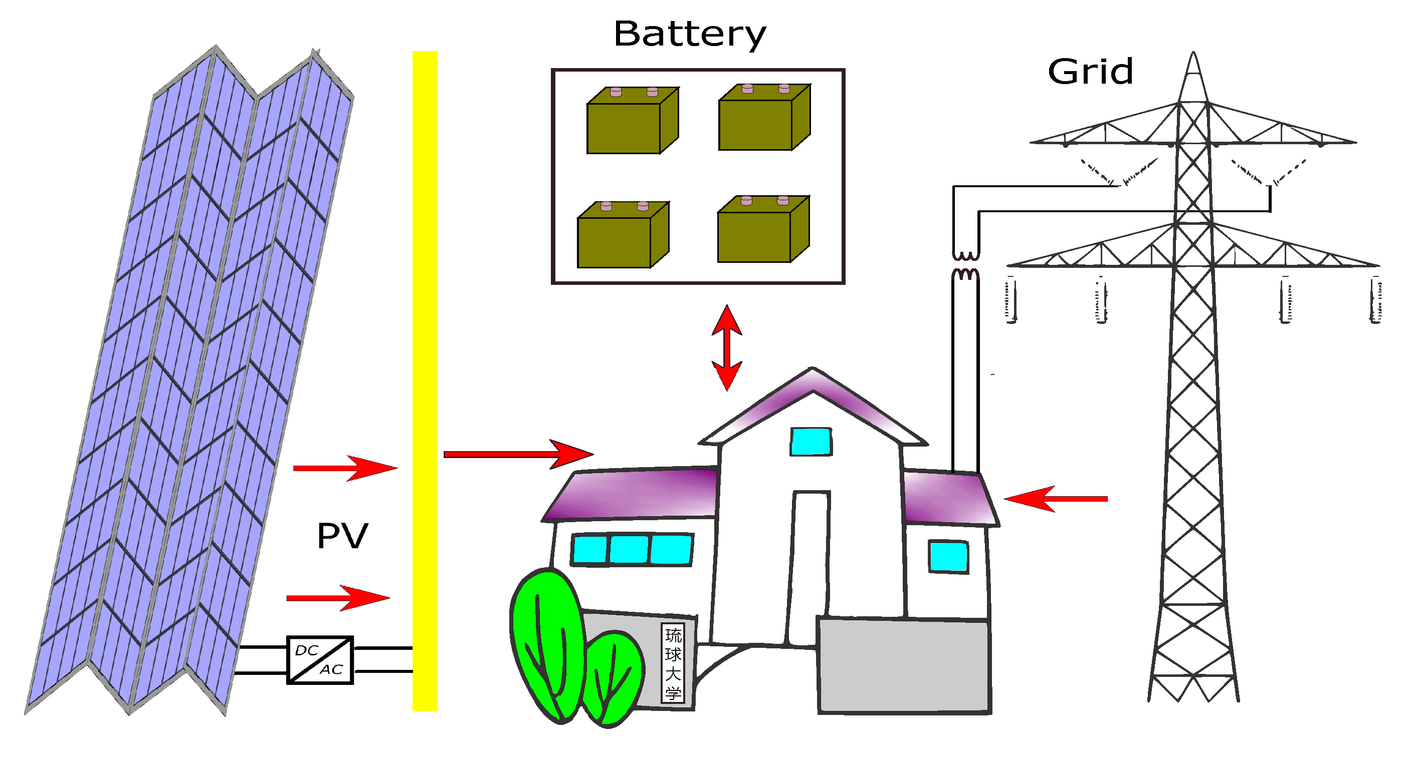
  • Based on the actual power load of University of the Ryukyus’s Senbaru Campus and the actual weather data in Okinawa, the optimal configuration of the combination of constant power from the grid, solar power, and storage size was used. According to the basic structure and characteristics of the solar/battery power generation system, we established the photovoltaic power generation and battery storage models to provide a basis for the optimal configuration of system capacity. Moreover, an in-depth analysis of the performance of the solar power generation system and a comprehensive system evaluation were used. The evaluation system included three indicators: loss of power supply probability, waste of energy, and total cost. This can evaluate the performance of the solar hybrid power generation system from various aspects such as system reliability and energy utilization. This article demonstrated a complete design of an optimized microgrid system.
  • Using the University campus as an example, the article showed the optimized combination of batteries, PV, and the grid that provided constant power, so that enterprises and institutions can reduce costs while eliminating the problem of peak power consumption. While energy conservation and emission reduction have been advocated, the amount of energy used every year is increasing [19]. When consumer satisfaction remains the primary priority without paying attention to the supply constraints, it is often difficult to reduce energy usage. Therefore, this article started from the user side, first stipulating the required energy considering the actual data and then allocating electricity demand. It avoided the traditional situation where the power supplier follows the consumer. The constant power sales program proposed in this paper provided a theoretical basis and practical reference for the stable operation of the microgrid.
The remainder of the article is structured as follows: Section 2 analyzes the mathematical models of various equipment. Section 3 provides the evaluation criteria of this system based on the electricity consumption of the University of Ryukyu in one year, formulating the optimization conditions and the optimization goals. Section 4 provides the details of the simulation results. Finally, Section 5 discusses the problems solved in this research and puts forward the remaining problems.

2. System Modeling and Optimization Method

The capacity configuration of the solar power generation system has a direct impact on the performance of the entire system. It is one of the critical contents of the system design. The capacity allocation of the micro-grid must first establish the power generation model of each power generation unit in the distributed power generation system. The actual data need to be used to obtain the amount of electricity that each power generation unit can reach. This section focuses on the analysis of two power supply units—photovoltaic panels and batteries—and establishes a methodology for the power generated by each power source to investigate the optimal configuration of the power generation system. Figure 1 shows the image of this PV system.

2.1. Photovoltaic Power Generation Model

The amount of PV power generation in a PV system depends on the solar radiance I r , the efficiency η of the PV module, and the quantity x 1 of the PV panels. It should be noted that shadows will affect the layout of solar panels, and the area was constrained here. Furthermore, the expanded floor area of each solar panel was considered, meaning there was an upper limit on the number of solar panels. By changing the traditional arrangement, the effective area can be greatly increased [20]. The M-shape refers to the solar panels facing east and west, and the overall look appears as a wave. Here, we considered the M-shaped arrangement method to arrange the PV array. According to the S-shaped array and the M-shape shown in Figure 2, the required area of the S-shaped and M-shaped area was calculated as follows. Formula (1) calculates the width of the gap. Formulas (2) and (3) calculate the footprint of each solar panel.
D a = L a × sin θ a tan α
S = W a × ( L a cos θ a + D a )
M = W a × L a cos θ b .
where D a is the space between panels (m), L a is the width of the panels (m), θ a is tilt angle of the panels ( ), α is the solar altitude angle ( ), W a is the length of the panels (m), and S and M respectively represent the area (m 2 ) of the two types [20].
The University of the Ryukyus Senbaru Campus has an area of 1,123,616 m 2 , and the building area occupies 186,307 m 2 [21]. The building area here was used as a constraint for the number of solar panels x 1 . Assuming the PV panels can be set on the roof of the University of the Ryukyus, through calculation, the S-shape can be set to 6800 and the M-shape to 12,000. The PV output power P p v can be derived from the following Formula (4):
P p v ( i ) = η × I r ( i ) × x 1 × M
where P p v is the PV output power (kW), η is the photoelectric conversion efficiency (%), I r is the solar radiation (kW/m 2 ), and x 1 is the number of solar panels, which is one of the optimal solutions we needed to find.

2.2. Battery Storage Model

Due to the dual-function—the discharge function and the energy storing capability—the batteries had a direct and important role in the stability of the power generation system. Compared with a hybrid micro-grid that does not use batteries, a system that uses batteries is more economical and reliable [22]. Here, the power generation P ( i ) from PV P p v ( i ) and grid P g ( i ) is given below in Formula (5).
P ( i ) = P p v ( i ) + P g ( i )
where P ( i ) is the total power available (kW), P p v is the power provided by PV (kW), and P g ( i ) is the unknown quantity x 3 , which is the power pre-purchased from the grid after the system is optimized (kW).

2.2.1. Charging

When the power generated by the hybrid system exceeds the power consumption of the load, the remaining power will be stored in the battery, and the battery will enter the charging state at this time. Here, the size of the battery x 2 is also the amount that needs to be optimized. However, as over-discharge or over-charge will affect the battery life [23], when the SOC of the battery is 80%, even if there is still excess power, the battery will not continue to store energy, but the energy is consumed through the unloading circuit. The calculation expression of the above process is as follows in Formula (6).
S O C ( i ) = S O C ( i 1 ) + [ P ( i ) L o a d ( i ) ] × γ x 2 , S O C ( i ) = m i n S O C ( i ) , x 2 × 80 % .

2.2.2. Discharging

When the power generation of the micro-grid system is less than the power required by the load, the battery will be used as a power source to supply power to the electrical load. When all the electric energy stored in the battery is discharged, the battery stops discharging, but the stored electric energy is 20% of the battery size x 2 . Surely, the system would not have enough power support at this moment. The calculation expression of the above process is as follows in Formula (7):
S O C ( i ) = S O C ( i 1 ) + [ P ( i ) L o a d ( i ) ] × γ x 2 , S O C ( i ) = m a x S O C ( i ) , x 2 × 20 % .

3. Simulation Conditions

The Sustainable Development Goals (SDG) adopted by the United Nations (UN) in September 2015 aim to achieve a better international society by solving global problems such as environmental degradation and poverty. The University of the Ryukyus, the case under study, sincerely agrees with these goals [24]. Therefore, the university seeks to design a reliable and tailored power system adopting clean energy resources. The combination of a large grid system and a distributed power generation system is a well-known approach to save the cost of investment, reduce energy consumption, and improve system safety and flexibility. Moreover, using the grid to provide constant power and large-sized battery banks makes the microgrid close to the stand-alone grid system. At the same time, pre-purchasing constant power can reduce the prediction pressure on the power station. The findings of this study can be of use to other institutions and universities in adopting such a microgrid system.
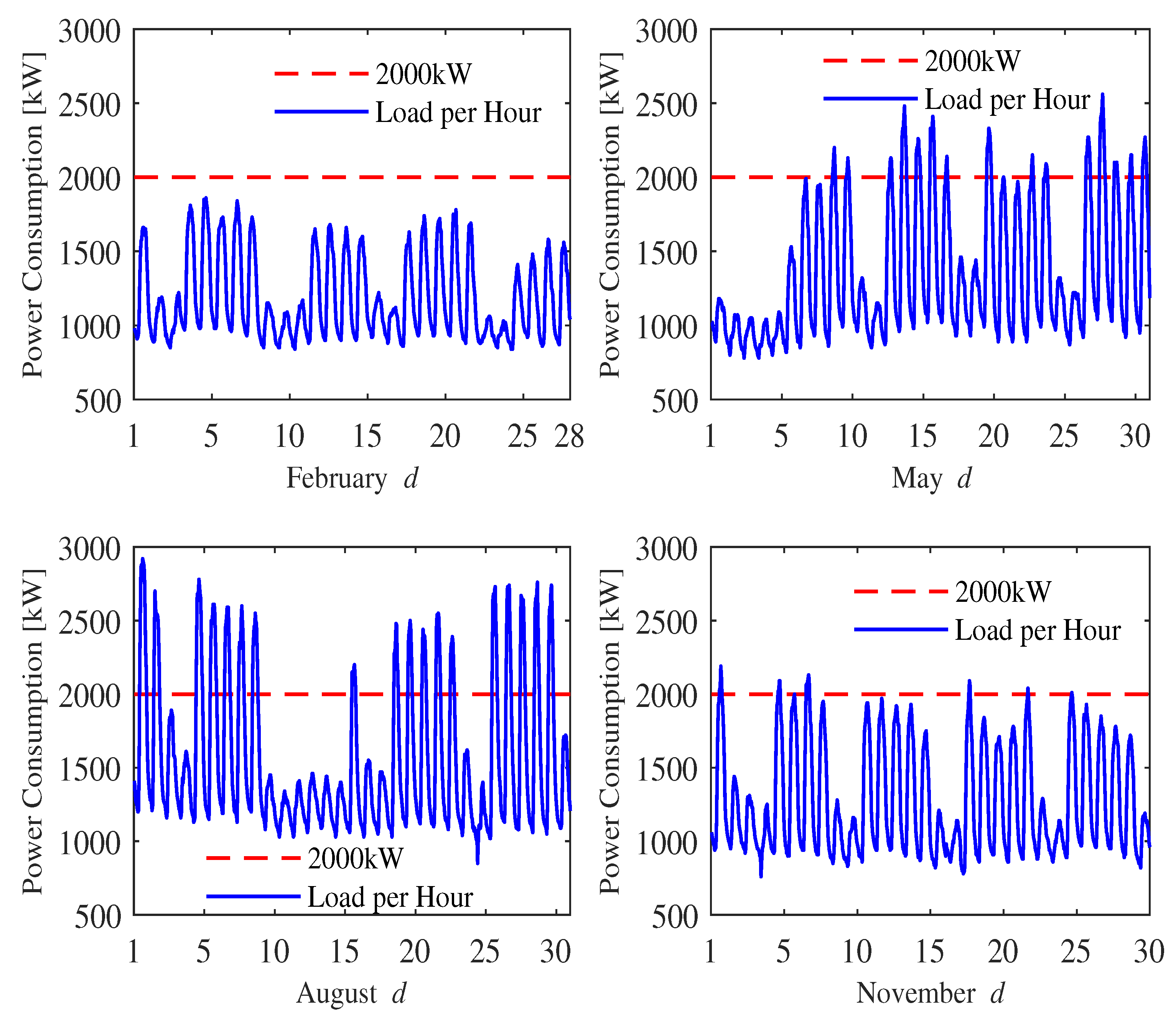
The partial electrical load of the University of the Ryukyus in 2019 is shown in Figure 3. The four months represent four quarters, although the seasons in Okinawa are variable. Figure 4 shows the boxplot of the University of the Ryukyus’ electricity consumption in 2019. First, the electricity consumption during workdays will be significantly higher than on other days. Second, there is a big difference between winter and summer. There were 16 days of peak load exceeding 2000 kW in May and 18 days of peak load exceeding 2000 kW in August. In February, the peak load was below 2000 kW, while in November, six days had more than 2000 kW of peak load. Third, the main load is from 9 a.m. to 9 p.m., which matches very well with solar power with only 3–4 h of deficit, except for cloudy or rainy days. Here, we considered the electricity commercial contract to provide fixed electricity every day. The reason for using constant power here was to consider the startup and shutdown of the peak-regulating generator at the power supply side. This will reduce fuel waste and labor costs. In Japan, inexpensive high-voltage electricity can be purchased from power companies, as mentioned by Tahara et al. [25]. Therefore, the electricity supply is obtained from the grid, which is less expensive than the regular market.
A reasonable evaluation system was proposed for various configurations of the PV system, which mainly included the following three indicators: loss of power supply probability (LPSP), waste of energy (WE), and life cycle cost (LCC). Hence, it can quantitatively calculate the system performance, and provides basic optimization goals for the optimal configuration of the solar power generation system.

3.1. Loss of Power Supply Probability

Reliability is the most basic requirement for power generation systems. The intermittency and variability of solar radiation will directly affect the power generation of the power generation system, which leads to reliability problems, which is particularly important in the solar power generation system. Here, reliability refers to the ability of the power generation system to provide continuous and sufficient power to the power load for a long time. The commonly used reliability evaluation index is the annual LPSP, which is defined as below. Formula (8) shows the total available power P T . Formula (9) shows if the supply meets 90% of the load in each hour (i). Formula (10) means the smaller the LPSP, the more reliable the system.
P T ( i ) = P p v ( i ) + P g ( i ) + P b a t ( i )
L P S ( i ) = 0 P T ( i ) L o a d ( i ) × 90 % 1 P T ( i ) < L o a d ( i ) × 90 %
L P S P = i = 1 N L P S ( i ) N

3.2. Waste of Energy

Due to factors such as the natural characteristics of solar energy, power generation cannot be guaranteed to be reasonable. It is necessary to evaluate the system’s ability to use renewable energy to improve the energy utilization rate of the power generation system. Therefore, this paper put forward the evaluation index of the WE to evaluate the energy utilization capacity of the system. It is defined as the unused electrical energy of the system during the whole year of operation divided by the total electrical energy generated by the system. The smaller the value, the higher the utilization rate of the system for renewable energy and the less energy wasted. The basic calculation process of WE is as Formula (11). Formula (12) adds up the amount of electricity each hour when the power support part exceeds the load.
W E ( i ) = 0 P T ( i ) L o a d ( i ) P T ( i ) L o a d ( i ) P T ( i ) > L o a d ( i )
W E = i = 1 N W E ( i )

3.3. Life Cycle Cost

The construction of any system must consider the cost input. For a solar power generation system, its cost is mainly composed of three parts: one-time investment cost, operation and maintenance cost, and component replacement cost. The one-time investment cost refers to the total purchase expenditure of all components in the system for the first time ( C u n i t ), which is mainly composed of the purchase cost of the three main power generation units in the power generation system. The operation and maintenance cost ( C O M ) includes mostly the yearly maintenance cost of each component in the system. The replacement cost ( C r e p ) is for the components that need to be replaced due to a short life span. They satisfy the following relationship, as shown in Formula (13).
L C C = C u n i t + C O M + C r e p
In order to consider the three necessary investment costs mentioned above and reduce the complexity of the cost calculation function used as much as possible, this article used a comprehensive cost function to calculate the system investment cost, which is defined as follows in Formula (14).
C u n i t = x 1 × C p v + x 2 × C b a t + x 3 × C g r i d
The PV operating and maintenance cost is shown as Formula (15).
C O M = x 1 × C p v × j p v = 1 19 1 + u p v 1 + v p v j p v
The price of the battery replacement cost is defined as the following Formula (16) (adding or replacing new batteries every five years).
C r e p = x 2 × C b a t × j b a t = 5 , 10 , 15 1 + u b a t 1 + v b a t j b a t
where C p v is the unit price of the photovoltaic panel, C b a t the unit price of the battery (kWh/JPY), C g r i d the electricity price (kWh/JPY), x 1 the number of PV panels, x 2 the size of the battery (kWh), x 3 the pre-purchased power (kWh), u the annual growth rate of replacement, v the interest rate, and j is life span of the battery or system [10].
The price of PV and battery modules are given in Table 1.

3.4. Optimization Goals and Constraints

Since solar power generation cannot provide the whole daily power demand of the campus, it is necessary to purchase electricity from the grid. This study developed and compared three cases. First, real-time electricity would be imported directly from the grid. Here, the price of the electricity company was set at 20 JPY/kWh. Second, the price for one year of pre-purchased constant power from the power company was set at 15 JPY/kWh ( 3 4 th of the original price). Third, the daily pre-purchased constant electricity price from the power company was also set at 15 JPY/kWh. However, in order to reduce power consumption as much as possible, when the purchased electricity exceeds 1000 kW/h, the price will be increased to 20 JPY/kWh, as shown in Formula (17). The carbon emission coefficient was defined as 0.769 kg/kWh [26].
C g r i d = 15 x 3 , x 3 1000 kWh / h 20 x 3 1000 , x 3 1500 kWh / h 25 x 3 1500 , x 3 2000 kWh / h
Hence, continuous and stable high-voltage electricity from the grid was purchased here. The main differences between the three cases are as follows.

3.4.1. Case 1

Obtain real-time power from the grid: O b j e c t 1 here was to find solutions that satisfy the Pareto front of W E and L C C , as shown in Formula (18).
O b j e c t 1 = f 1 ( x 1 , x 2 )
O b j e c t 1 = min ( W E , L C C ) s . t . 0 x 1 1000 0 x 2 12,000

3.4.2. Case 2

Pre-purchase one year of constant power x 3 : O b j e c t 2 here was to find solutions that satisfy the Pareto front of W E , L C C , and L S P S , as shown in Formula (19).
O b j e c t 2 = f 2 ( x 1 , x 2 , x 3 )
O b j e c t 2 = min ( L S P S , W E , L C C ) s . t . 0 x 1 1000 0 x 2 12,000 1000 x 3 1500

3.4.3. Case 3

Pre-order daily constant power X: This is the same objective as Case 2 as shown in Formula (20). Specifically, Formula (21) was used in Case 3 as a reference indicator for the daily power required.
O b j e c t 2 = f 2 ( x 1 , x 2 , X )
O b j e c t 2 = min ( L P S P , W E , L C C ) s . t . 0 x 1 1000 0 x 2 12,000 X ( p e r H ± 50 )
p e r H = i = 1 24 ( L o a d ( i ) P V ( i ) ) 24
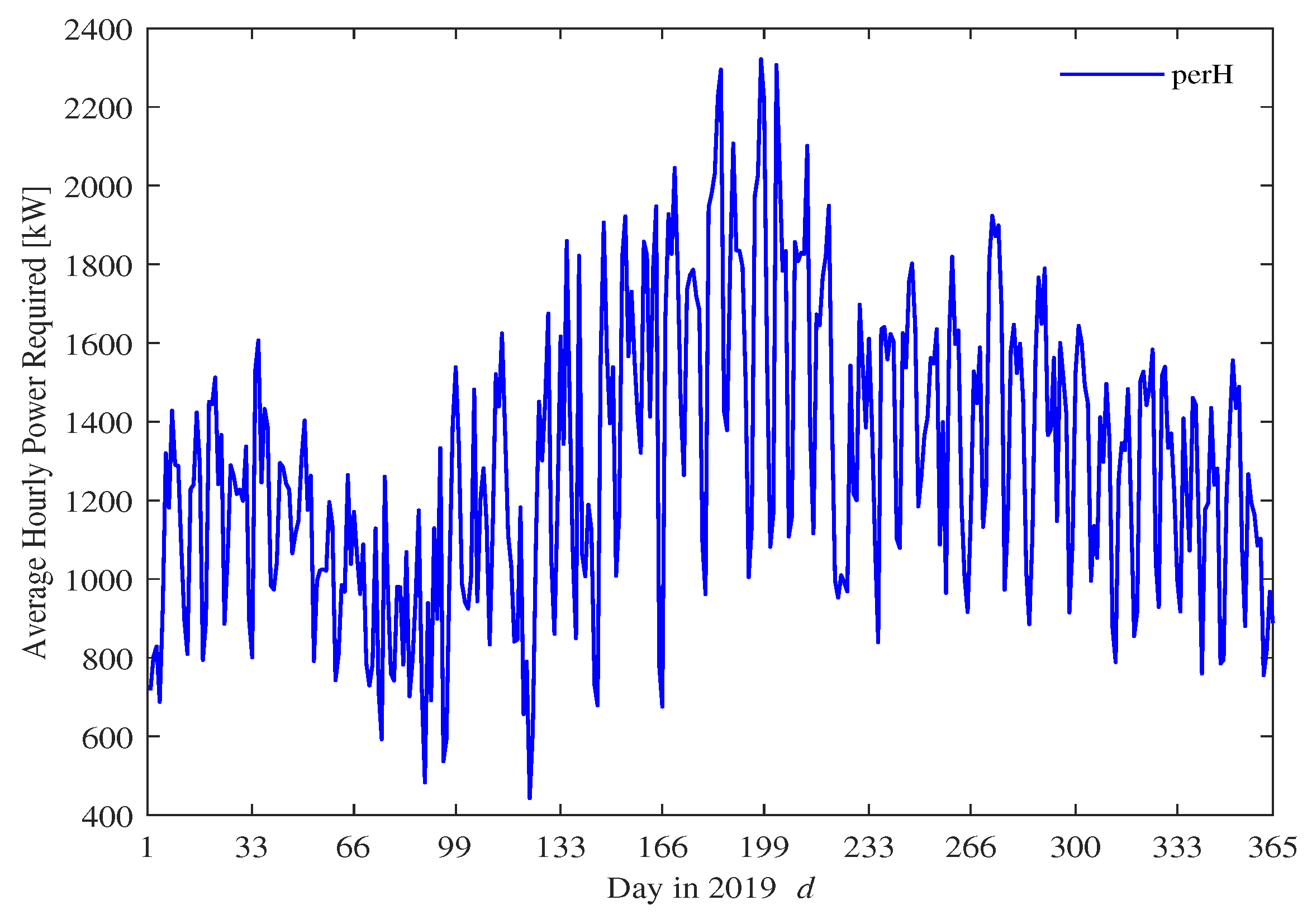
The total daily electricity consumption minus the electricity generated by PV was used to calculate the average electricity consumption during the day. Figure 5 shows the result of the calculated value p e r H . Figure 6 is an example without the X ( p e r H ± 50 ) range.

4. Simulation Results and Discussion

From the perspective of the development trend of electric vehicles, in the future work, combined with the following results, It is believe that if the orderly charging and discharging of electric vehicles is considered in the campus microgrid, the feasibility of this scheme will be higher.
In Case 1, when selecting the Pareto solution, the best solution was selected, that is the solution that stood out from the curve. In Cases 2 and 3, we followed the same selection method as Case 1, but three comparisons were required. After each comparison was determined, the solutions that were not optimized enough were excluded, and the next round of comparisons was performed.

4.1. Case 1

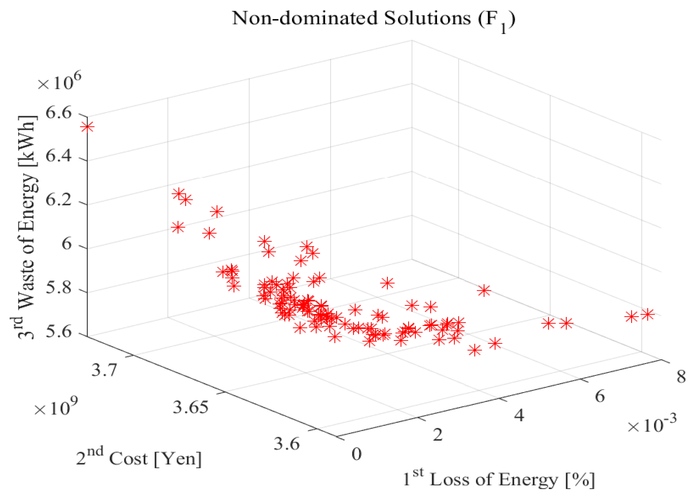
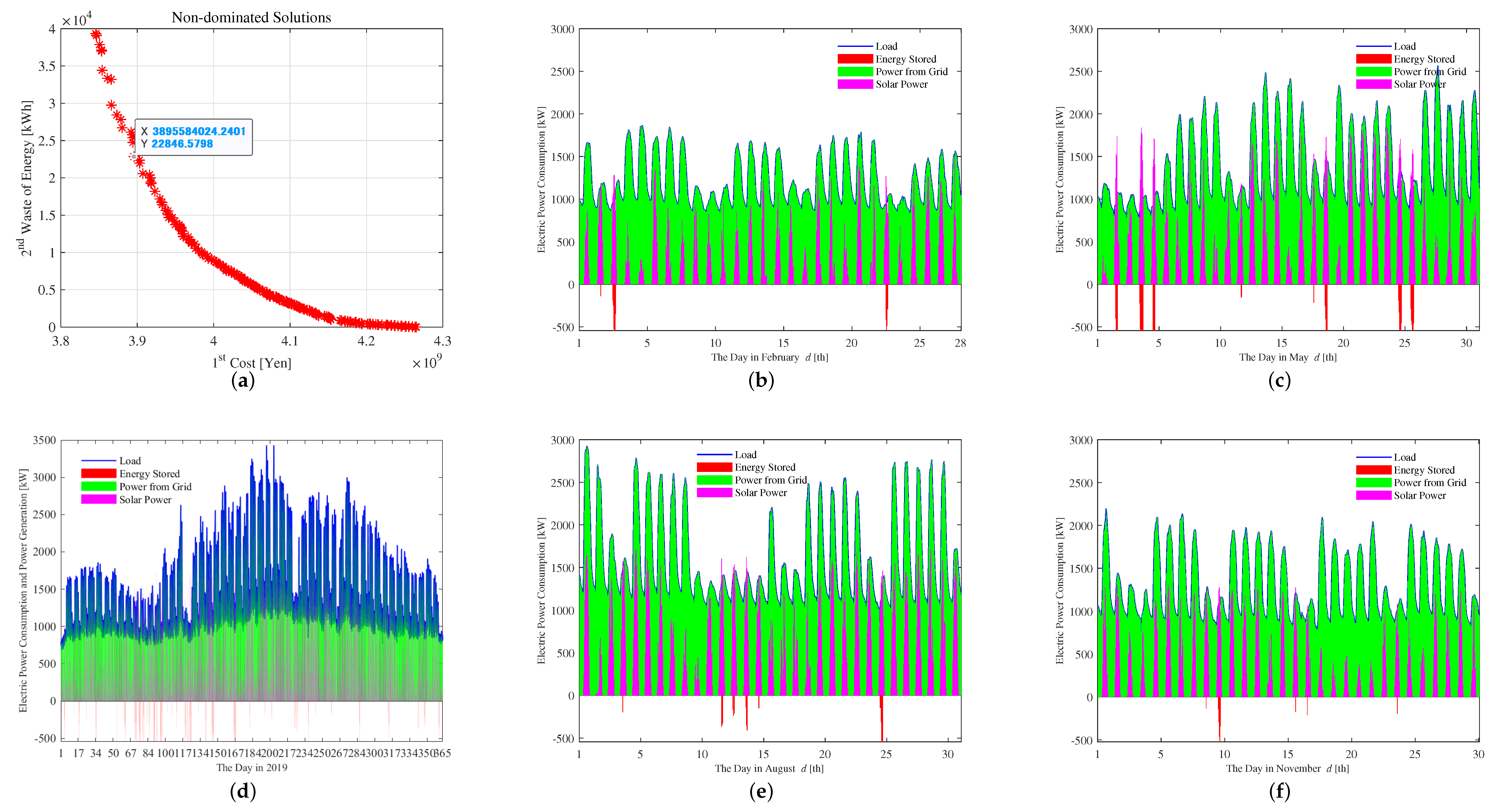
Figure 7a shows the Pareto front between the electricity bill and wasted energy and diagrams of the power generation and power consumption in February (b), May (c), August (e), November (f), and the whole year (d). It can be found from Pareto front that the electricity cost was about 3.90 × 10 9 JPY and the energy wasted was 22,847 kW. The number of solar panels and the size of the battery are shown in Table 2. The green part in the figure is the power obtained from the grid. The red part is the energy stored in the battery. The magenta part is the solar energy, due to the large number of solar panels, which was also greatly affected by sun radiation. This part of the electrical energy can competently cope with the peak power consumption of universities. However, even energy waste caused by intense radiation. In this simulation, the red part in the figure would appear a bit redundant. Due to this case considering that a steady stream of electric energy can be obtained from the grid, the battery can only collect the occasional excess energy.
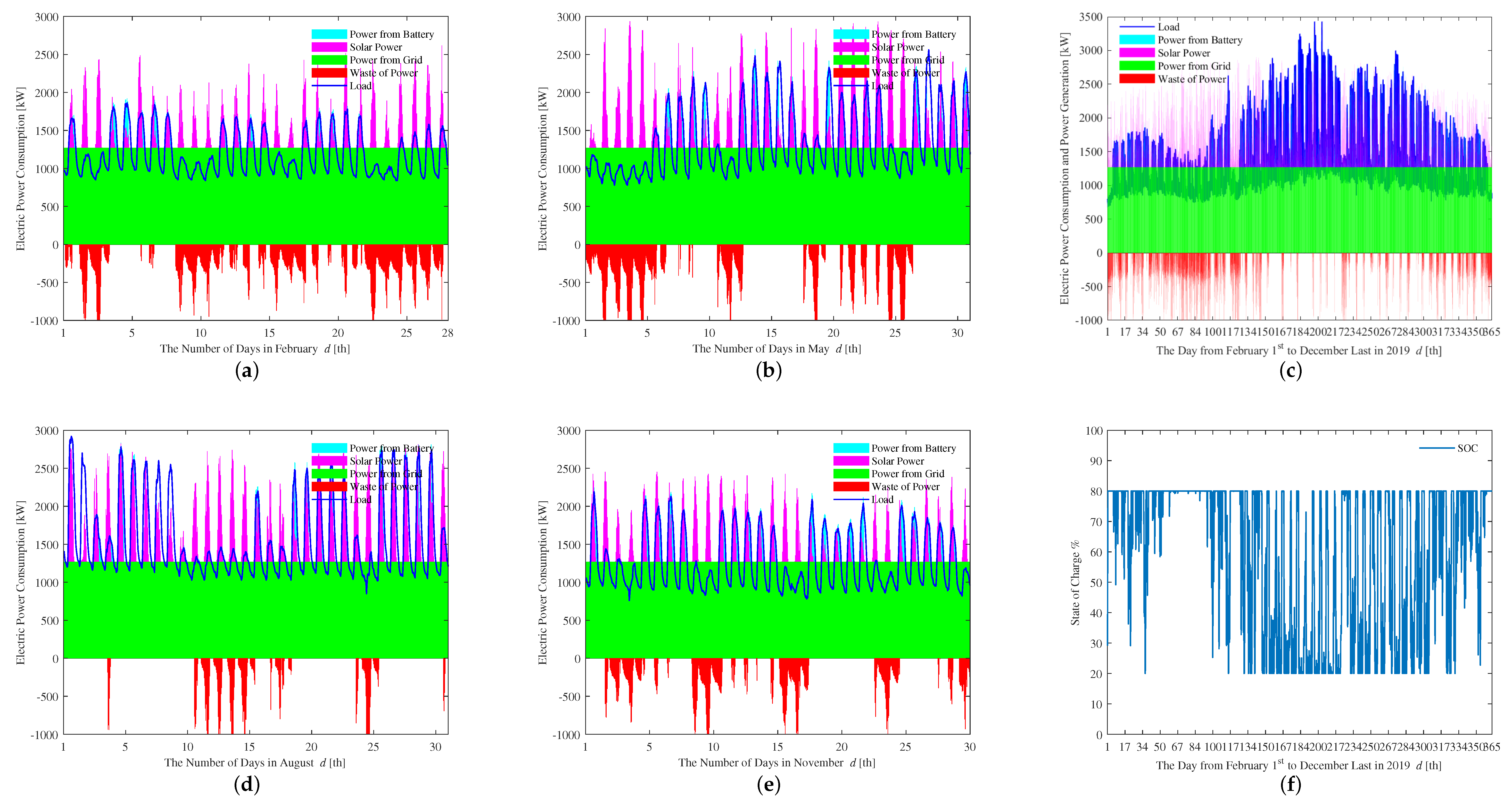
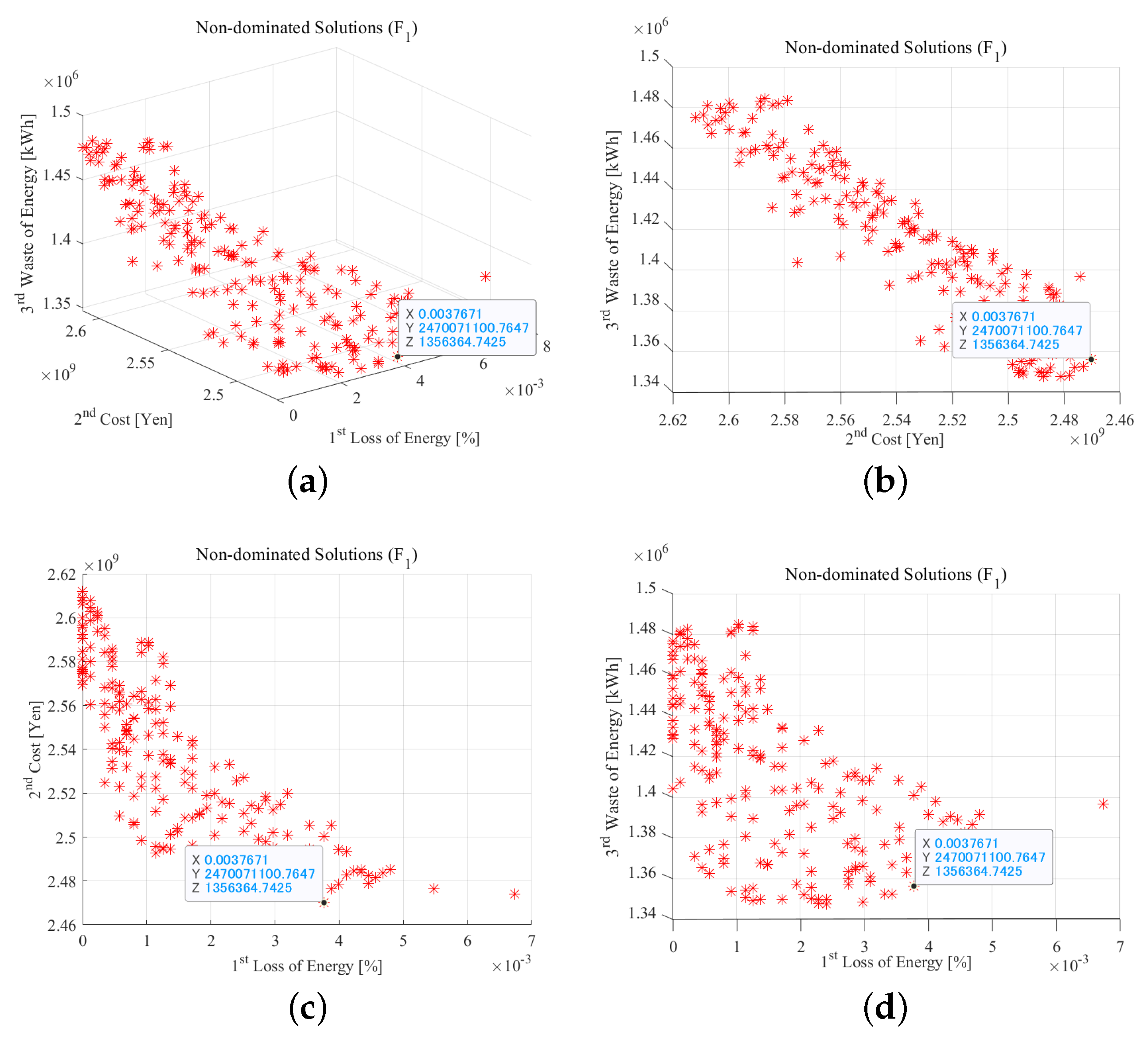
4.2. Case 2

Figure 8 shows the Pareto relationship between lost energy, cost, and wasted energy. Here, we used a solution that costs 2.45 × 10 9 JPY. Among these, the battery size was 796 kW; the usage of the solar panels was 10,636 kW; and the constant electric energy for every hour was 1270 kW, as shown in 
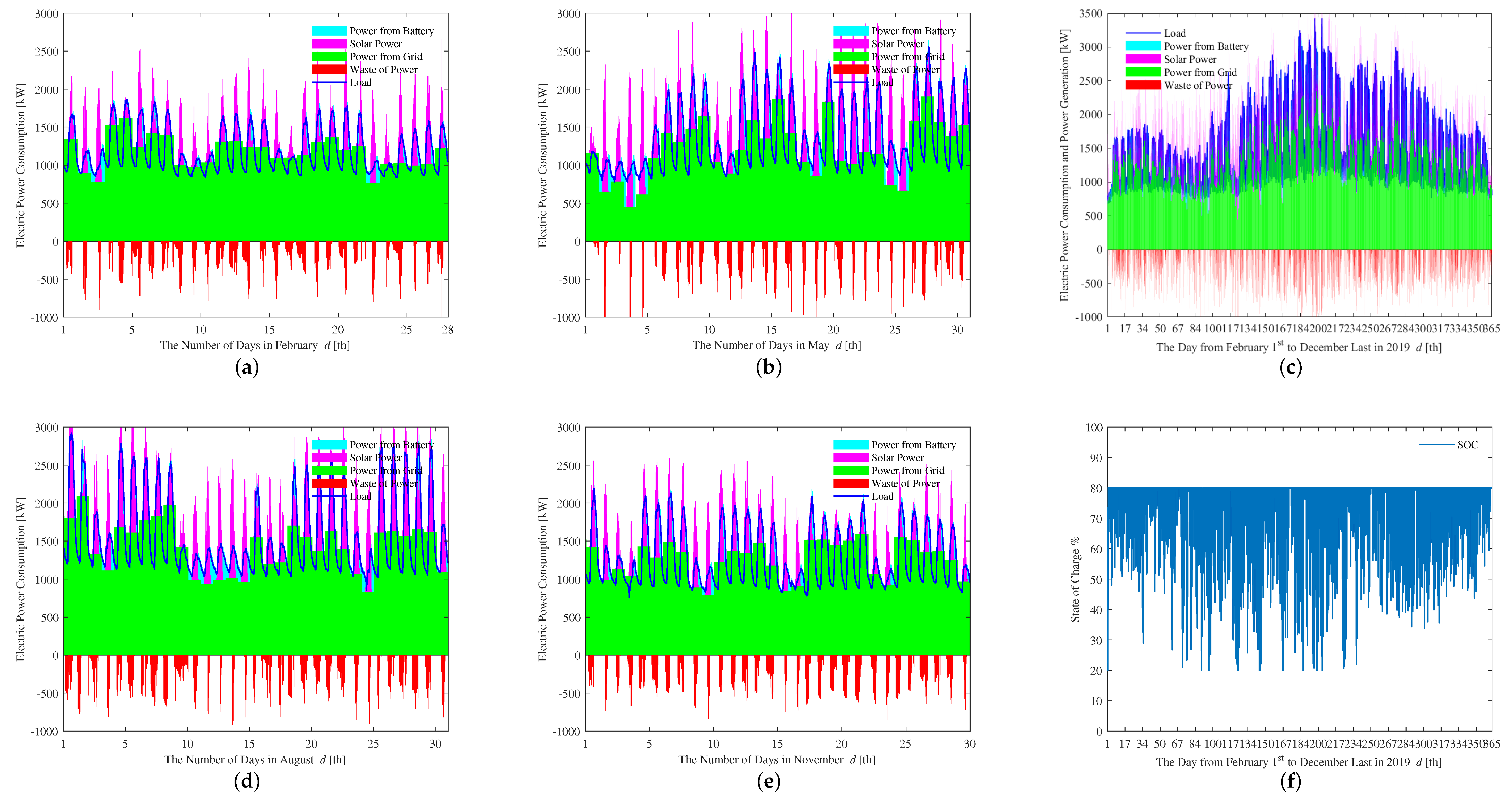
Table 3. Here, we use the LPSP as the reference standard for this power operation plan. When it was less than 0.05%, we considered the solutions to be reliable. Compared with Case 1, using this solution would waste more energy, and it was also challenging to obtain 100% real-time power support and lower costs. From another perspective, this wasted energy can be regarded as having potential value waiting to be developed.
Figure 9 shows the battery SOC for the four seasons. There were many periods when the battery was fully charged or discharged such as: 20–28 February; 1–5 May; 10–15 August; 2–5 November. This shows that the battery was not fully utilized here. Although this can protect the battery, the article considered the cost of replacing the battery once every five years as in Formula (16). Therefore, a third option was proposed in Case 3.
Figure 10 shows the corresponding power generation and power usage in the four seasons, the whole year, and one year of the SOC of the battery bank. The green part is the constant electricity obtained from the grid. Although green occupies a large part, it is difficult to solve these issues. It can be found from the figure that the magenta part protects the peak power of the campus. However, the problem is that this part of the electricity is difficult to consume during the other days. Corresponding to this are the red parts, which represent wasted energy. It can also be found in the figure that in summer, energy waste is less than in spring. From the 50th day to the 100th day, the battery can be regarded as unused. Here, dividing power purchases into summer and spring categories will give better results.

4.3. Case 3

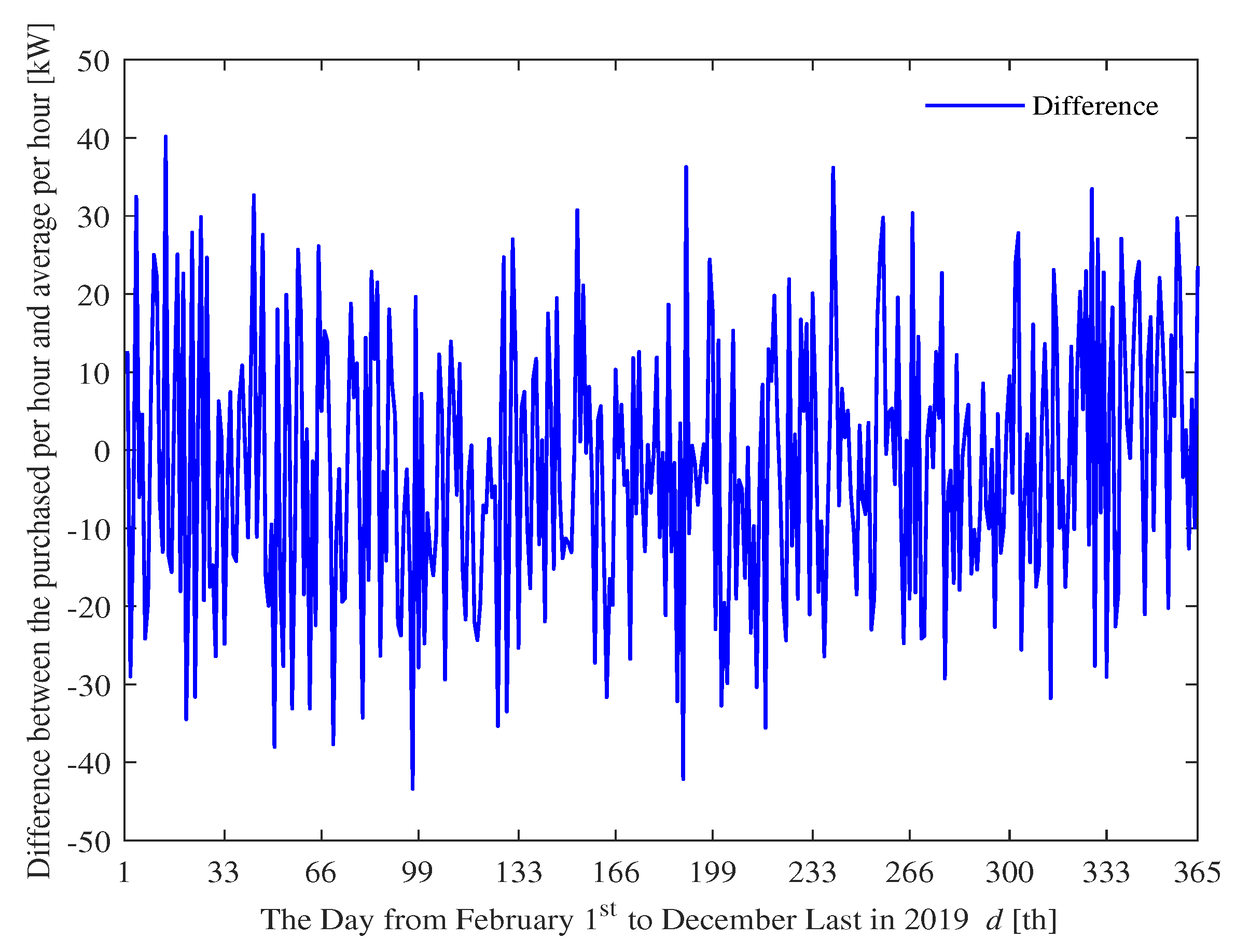
Figure 11 is the difference between the purchased power X and the average power required per hour per day, as shown in Figure 5.
Figure 12 gives the Pareto solutions of Case 3. The selected solution is shown in Table 4. Because all the LPSPs in this Pareto front were less than 0.5%, we chose the one with the lowest cost. Figure 12c shows the comparison of Case 2 (Figure 10) and Case 3 (Figure 14), showing that the red part in the Case 3 scheme is more stable. This shows that the energy of Case 3 can be more easily used.
Figure 13 shows that the battery had a relatively high number of charge and discharge times and was used often. Figure 14 shows the same items as Figure 10, but in comparison, the line density in Figure 14 shows more regularity. It also shows that the feasibility of Case 3 is higher.
The results of the three cases are shown in Table 5. From the results, it can be found that the cost would be greatly reduced for Cases 2 and 3 compared to Case 1. From the perspective of carbon emissions and wasted energy, Case 2 obtained less power from the grid than Case 3, but it wasted more electricity. It can be seen that the main waste was the electricity generated by PV. If this part of the energy can be converted into heat and stored, this would lower the LPSP. The electrical energy of Case 3 was more useful for electric vehicle charging stations, especially in places similar to Okinawa where car usage is important.

5. Conclusions

This paper used NSGA-II optimization to optimize the power supply system under three conditions. According to the findings, purchasing one year of constant power was less expensive, and the wasted energy in Case 3 was more reusable. The original intention of this paper was to design a power supply system that used clean energy as much as possible for the University, which would reduce dependence on the grid. In these three cases, the carbon emissions of Case 1 were the smallest followed by Case 2 and Case 3; but their effects on grid stability were very different. The simulation in the article was reliable under the guarantee of the LPSP (under 0.05%). Moreover, in terms of wasted energy and the cost of energy, Cases 2 and 3 were obviously different from Case 1. This showed that the pre-purchasing of constant fixed power was more favorable than the general electricity grid connection for universities or some enterprise institutions that use electricity during the day.

Author Contributions

Conceptualization, Y.H. and H.M.; methodology, Y.H.; software, Y.H.; validation, Y.H., H.M. and R.S.; formal analysis, Y.H.; investigation, Y.H.; resources, Y.H.; data curation, Y.H.; writing—original draft preparation, Y.H. and H.M.; writing—review and editing, Y.H., H.M., R.S., A.M.H. and A.M.; visualization, H.M.; supervision, T.S.; project administration, T.S. and H.M.; funding acquisition, T.S. All authors read and agreed to the published version of the manuscript.

Funding

This research received no external funding.

Institutional Review Board Statement

Not applicable.

Informed Consent Statement

Not applicable.

Data Availability Statement

Not applicable.

Acknowledgments

The authors thankfully acknowledge the support of the authority of the University of the Ryukyus for providing the necessary data. The authors also gratefully acknowledge Harun Or Rashid Howlader for the insightful discussions throughout the course of this article.

Conflicts of Interest

The authors declare no conflict of interest.

Abbreviations

The following abbreviations are used in this manuscript:
PVPhotovoltaic
NSGA-IINon-dominated sorting genetic algorithm II
LPSPLoss of power supply probability
LCCLife cycle cost
WEWaste of energy
ESSEnergy storage systems
GAGenetic algorithm
HESsHybrid energy systems
nZEBNearly/net-zero energy buildings
CSEAChaotic self-adaptive evolutionary algorithm
WGWind turbine
BESSBattery energy storage system
FCFuel cell
MILPMixed-integer linear programming
SOCState of charge
SDGSustainable Development Goals
UNUnited Nations

References

  1. Nehrir, M.H.; Wang, C.; Strunz, K.; Aki, H.; Ramakumar, R.; Bing, J.; Miao, Z.; Salameh, Z. A Review of Hybrid Renewable/Alternative Energy Systems for Electric Power Generation: Configurations, Control, and Applications. IEEE Trans. Sustain. Energy 2011, 2, 392–403. [Google Scholar] [CrossRef]
  2. Mohandes, B.; Moursi, M.S.E.; Hatziargyriou, N.; Khatib, S.E. A Review of Power System Flexibility with High Penetration of Renewables. IEEE Trans. Power Syst. 2019, 34, 3140–3155. [Google Scholar] [CrossRef]
  3. Eid, B.M.; Rahim, N.A.; Selvaraj, J.; Khateb, A.H.E. Control Methods and Objectives for Electronically Coupled Distributed Energy Resources in Microgrids: A Review. IEEE Syst. J. 2014, 10, 446–458. [Google Scholar] [CrossRef]
  4. Hossain, E.; Kabalci, E.; Bayindir, R.; Perez, R. Microgrid testbeds around the world: State of art. Energy Convers. Manag. 2014, 86, 132–153. [Google Scholar] [CrossRef]
  5. Hosenuzzaman, M.; Rahim, N.; Selvaraj, J.; Hasanuzzaman, M.; Malek, A.A.; Nahar, A. Global prospects, progress, policies, and environmental impact of solar photovoltaic power generation. Renew. Sustain. Energy Rev. 2015, 41, 284–297. [Google Scholar] [CrossRef]
  6. Masrur, H.; Senjyu, T.; Islam, M.R.; Kouzani, A.Z.; Mahmud, M.A.P. Optimal Operation of Resilient Microgrids During Grid Outages. In Proceedings of the 2020 IEEE International Conference on Applied Superconductivity and Electromagnetic Devices (ASEMD), Tianjin, China, 16–18 October 2020; pp. 1–2. [Google Scholar] [CrossRef]
  7. Arefin, A.A.; Masrur, H.; Othman, M.L.; Hizam, H.; Abdul Wahab, N.I.; Jalaluddin, N.A.; Islam, S.Z. Power Resilience Enhancement of a PV-Battery-Diesel Microgrid. In Proceedings of the 2020 International Conference on Smart Grids and Energy Systems (SGES), Perth, Australia, 23–26 November 2020; pp. 860–863. [Google Scholar] [CrossRef]
  8. Barbour, E.; Parra, D.; Awwad, Z.; González, M.C. Community energy storage: A smart choice for the smart grid? Appl. Energy 2018, 212, 489–497. [Google Scholar] [CrossRef] [Green Version]
  9. Bracco, S.; Brignone, M.; Delfino, F.; Procopio, R. An Energy Management System for the Savona Campus Smart Polygeneration Microgrid. IEEE Syst. J. 2015, 11, 1799–1809. [Google Scholar] [CrossRef]
  10. Sediqi, M.M.; Furukakoi, M.; Lotfy, M.E.; Yona, A.; Senjyu, T. Optimal economical sizing of grid-connected hybrid renewable energy system. J. Energy Power Eng. 2017, 11, 244–253. [Google Scholar]
  11. Huang, Z.; Lu, Y.; Wei, M.; Liu, J. Performance analysis of optimal designed hybrid energy systems for grid-connected nearly/net zero energy buildings. Energy 2017, 141, 1795–1809. [Google Scholar] [CrossRef]
  12. Masrur, H.; Howlader, H.O.R.; Elsayed Lotfy, M.; Khan, K.R.; Guerrero, J.M.; Senjyu, T. Analysis of Techno-Economic-Environmental Suitability of an Isolated Microgrid System Located in a Remote Island of Bangladesh. Sustainability 2020, 12, 2880. [Google Scholar] [CrossRef] [Green Version]
  13. Konneh, K.V.; Masrur, H.; Othman, M.L.; Wahab, N.I.A.; Hizam, H.; Islam, S.Z.; Crossley, P.; Senjyu, T. Optimal Design and Performance Analysis of a Hybrid Off-Grid Renewable Power System Considering Different Component Scheduling, PV Modules, and Solar Tracking Systems. IEEE Access 2021, 9, 64393–64413. [Google Scholar] [CrossRef]
  14. Howlader, H.O.R.; Sediqi, M.M.; Ibrahimi, A.M.; Senjyu, T. Optimal thermal unit commitment for solving duck curve problem by introducing CSP, PSH and demand response. IEEE Access 2018, 6, 4834–4844. [Google Scholar] [CrossRef]
  15. Song, H. Multi-objective optimal sizing of stand-alone hybrid wind/PV system. Diangong Jishu Xuebao (Trans. China Electrotech. Soc.) 2011, 26, 104–111. [Google Scholar]
  16. Mehrjerdi, H.; Bornapour, M.; Hemmati, R.; Ghiasi, S.M.S. Unified energy management and load control in building equipped with wind-solar-battery incorporating electric and hydrogen vehicles under both connected to the grid and islanding modes. Energy 2019, 168, 919–930. [Google Scholar] [CrossRef]
  17. Gamil, M.M.; Sugimura, M.; Nakadomari, A.; Senjyu, T.; Howlader, H.O.R.; Takahashi, H.; Hemeida, A.M. Optimal Sizing of a Real Remote Japanese Microgrid with Sea Water Electrolysis Plant Under Time-Based Demand Response Programs. Energies 2020, 13, 3666. [Google Scholar] [CrossRef]
  18. Susowake, Y.; Masrur, H.; Yabiku, T.; Senjyu, T.; Motin Howlader, A.; Abdel-Akher, M.; M. Hemeida, A. A Multi-Objective Optimization Approach towards a Proposed Smart Apartment with Demand-Response in Japan. Energies 2019, 13, 127. [Google Scholar] [CrossRef] [Green Version]
  19. CO2 Emissions by Energy Source, World 1990–2018. Available online: https://www.iea.org/data-and-statistics/data-browser/?country=WORLD&fuel=CO2%20emissions&indicator=CO2BySource (accessed on 7 May 2021).
  20. Huang, Y.; Shigenobu, R.; Yona, A.; Mandal, P.; Yan, Z.; Senjyu, T. M-Shape PV Arrangement for Improving Solar Power Generation Efficiency. Appl. Sci. 2020, 10, 537. [Google Scholar] [CrossRef] [Green Version]
  21. University of the Ryukyus Data Book. 2019. Available online: https://www.u-ryukyu.ac.jp/wp-content/uploads/2020/01/632c54fb8d40a1dbb7aaefbef5199966.pdf (accessed on 29 July 2020).
  22. Belfkira, R.; Zhang, L.; Barakat, G. Optimal sizing study of hybrid wind/PV/diesel power generation unit. Sol. Energy 2011, 85, 100–110. [Google Scholar] [CrossRef]
  23. Yang, X.; Dong, D.; Xiangjun, L.I.; Xue, M.A.; Geng, N.; Jia, X. Active Power Coordinated Control Strategy of Peak Load Shifting for Energy Storage System in Business Park. Power Syst. Technol. 2018, 42, 2551–2561. [Google Scholar]
  24. Initiatives for SDGs at the University of the Ryukyus. Available online: https://www.u-ryukyu.ac.jp/aboutus/sdgs/ (accessed on 29 July 2020).
  25. Tahara, H.; Matayoshi, H.; Howlader, H.O.R.; Aditya, S.; Senjyu, T. Smart Apartment with Demand-Response Andfixed Batteries. In Proceedings of the 14th Conference of International Building Performance Simulation Association (BS 2015), Hyderabad, India, 7–9 December 2015; pp. 2587–2592. [Google Scholar]
  26. A Public Table of Basic Emission Coefficients, Adjusted Emission Coefficients of the Electric Company in Heisei 30. Available online: http://www.env.go.jp/press/107541-print.html (accessed on 10 October 2020).
Figure 1. The proposed micro-grid system model.
Energies 14 02853 g001
Figure 2. Schematic diagram of S- and M-shaped PV arrangement [20]. (a) S-shaped PV arrangement schematic; (b) M-shaped PV arrangement schematic.
Energies 14 02853 g002
Figure 3. Electricity consumption of the University of the Ryukyus in four different months in 2019.
Energies 14 02853 g003
Figure 4. Electricity consumption of the University of the Ryukyus in 2019.
Energies 14 02853 g004
Figure 5. Average power required per hour per day.
Energies 14 02853 g005
Figure 6. Failed Pareto front of Case 3.
Energies 14 02853 g006
Figure 7. Pareto front and simulation results of Case 1. (a) Pareto front of Case 1; (b) Simulation result of February; (c) Simulation result of May; (d) Simulation result of the whole year; (e) Simulation result of August; (f) Simulation result of November.
Energies 14 02853 g007
Figure 8. Pareto front results of Case 2. (a) 3D Pareto front; (b) Pareto front with LCC and WE; (c) Pareto front with LSPS and LCC; (d) Pareto front with LSPS and WE.
Energies 14 02853 g008
Figure 9. SOC of Case 2 for 4 months.
Energies 14 02853 g009
Figure 10. Simulation result of Case 2. (a) Simulation result of February; (b) Simulation result of May; (c) Simulation result of the whole year; (d) Simulation result of Augus; (e) Simulation result of November; (f) Simulation result of the whole year’s SOC.
Energies 14 02853 g010
Figure 11. The disparity between the purchased power and the average daily power needed.
Energies 14 02853 g011
Figure 12. Pareto front results of Case 3. (a) 3D Pareto front; (b) Pareto front with LCC and WE; (c) Pareto front with LSPS and LCC; (d) Pareto front with LSPS and WE.
Energies 14 02853 g012
Figure 13. SOC of Case 3 for 4 months.
Energies 14 02853 g013
Figure 14. Simulation result of Case 3. (a) Simulation result of February; (b) Simulation result of May; (c) Simulation result of the whole year; (d) Simulation result of August; (e) Simulation result of November; (f) Simulation result of the whole year’s SOC.
Energies 14 02853 g014
Table 1. Price of units.
IndexUnit PriceLife Span
PV10,000 (JPY/Module)20 (Year)
Battery15,000 (JPY/kWh)5 (Year)
Table 2. Solution of Case 1.
Case 1Battery (kWh)PV (Module)
Solution6811,736
Table 3. Solution of Case 2.
Case 2Battery (kWh)PV (Module)Grid (kWh)
Solution79610,6361270
Table 4. Solution of Case 3.
Case 3Battery (kWh)PV (Module)Grid (kWh)
Solution59111,320X
Table 5. Comparison of the three cases.
IndicatorCase 1Case 2Case 3
L P S P [ % ] /0.04720.0038
W E [ k W h ] 2.28 × 10 4 1.60 × 10 6 1.36 × 10 6
L C C [ J P Y ] 3.90 × 10 9 2.45 × 10 9 2.47 × 10 9
C O 2 [ t C O 2 ] 1.45 × 10 5 1.71 × 10 5 1.74 × 10 5
Publisher’s Note: MDPI stays neutral with regard to jurisdictional claims in published maps and institutional affiliations.

