Thermal and Flow Simulation of Concentric Annular Heat Pipe with Symmetric or Asymmetric Condenser

Abstract

The current research work describes the flow and thermal analysis inside the circular flow region of an annular heat pipe with a working fluid, using computational fluid dynamics (CFD) simulation. A two-phase flow involving simultaneous evaporation and condensation phenomena in a concentric annular heat pipe (CAHP) is modeled. To simulate the interaction between these phases, the volume of fluid (VOF) technique is used. The temperature profile predicted using computational fluid dynamics (CFD) in the CAHP was compared with previously obtained experimental results. Two-dimensional and three-dimensional simulations were carried out, in order to verify the usefulness of 3D modeling. Our goal was to compute the flow characteristics, temperature distribution, and velocity field inside the CAHP. Depending on the shape of the annular heat pipe, the thermal performance can be improved through the optimal design of components, such as the inner width of the annular heat pipe, the location of the condensation part, and the amount of working fluid. To evaluate the thermal performance of a CAHP, a numerical simulation of a 50 mm long stainless steel CAHP (1.1 and 1.3 in diameter ratio and fixed inner tube diameter (78 mm)) was done, which was identical to the experimental system. In the simulated analysis results, similar results to the experiment were obtained, and it was confirmed that the heat dissipation was higher than that of the existing conventional heat pipe, where the heat transfer performance was improved when the asymmetric area was cooled. Moreover, the simulation results were validated using the experimental results. The 3-D simulation shows good agreement with the experimental results to a reasonable degree.

1. Introduction

In the new era of high-performance electronics technology for future electric vehicle and personal applications, the minimization of high-performance electronics can lead to high energy consumption and high heat dissipation rates, allowing for efficient thermal management. The necessity for high-performance passive thermal management devices for use in electronics can be satisfied by heat pipes. A heat pipe is a passive two-phase heat transfer device, which can solve a wide range of thermal management problems at different levels of packaging. Even though heat pipes have been widely studied by researchers, most of the work has been restricted to experimental research, due to the difficulties in modeling the two-phase flow phenomena inside. A heat pipe consists of a suitable amount of working fluid in a metallic vacuum space and is operated using the latent heat of the working fluid. When the evaporator section is heated, the liquid inside changes into the vapor phase and transfers heat to the other side, the condenser section, by latent heat movement. In the condenser section, which passes through the adiabatic section, the vapor changes phase into a liquid through external cooling. The changed liquid is operated repeatedly, by returning it to the evaporator through various forms of force using the capillary force, gravity, centrifugal force, electrostatic force, osmotic pressure, and so on, of the wick. Heat pipes generally have a thermal conductivity superior to copper’s thermal conductivity of 400 W/m∙K and are durable enough to be used for more than 15 years [1,2,3,4,5].

In addition, the operating temperature of the heat pipe is in the cryogenic to high temperature range; that is, from −271 °C to 2200 °C [3]. Heat pipes demonstrate highly efficient heat transfer performance and excellent durability and have been used and studied in a wide range of applications in space, as well as for waste heat recovery from industrial plants or for the heating and cooling of small electronic components [4].

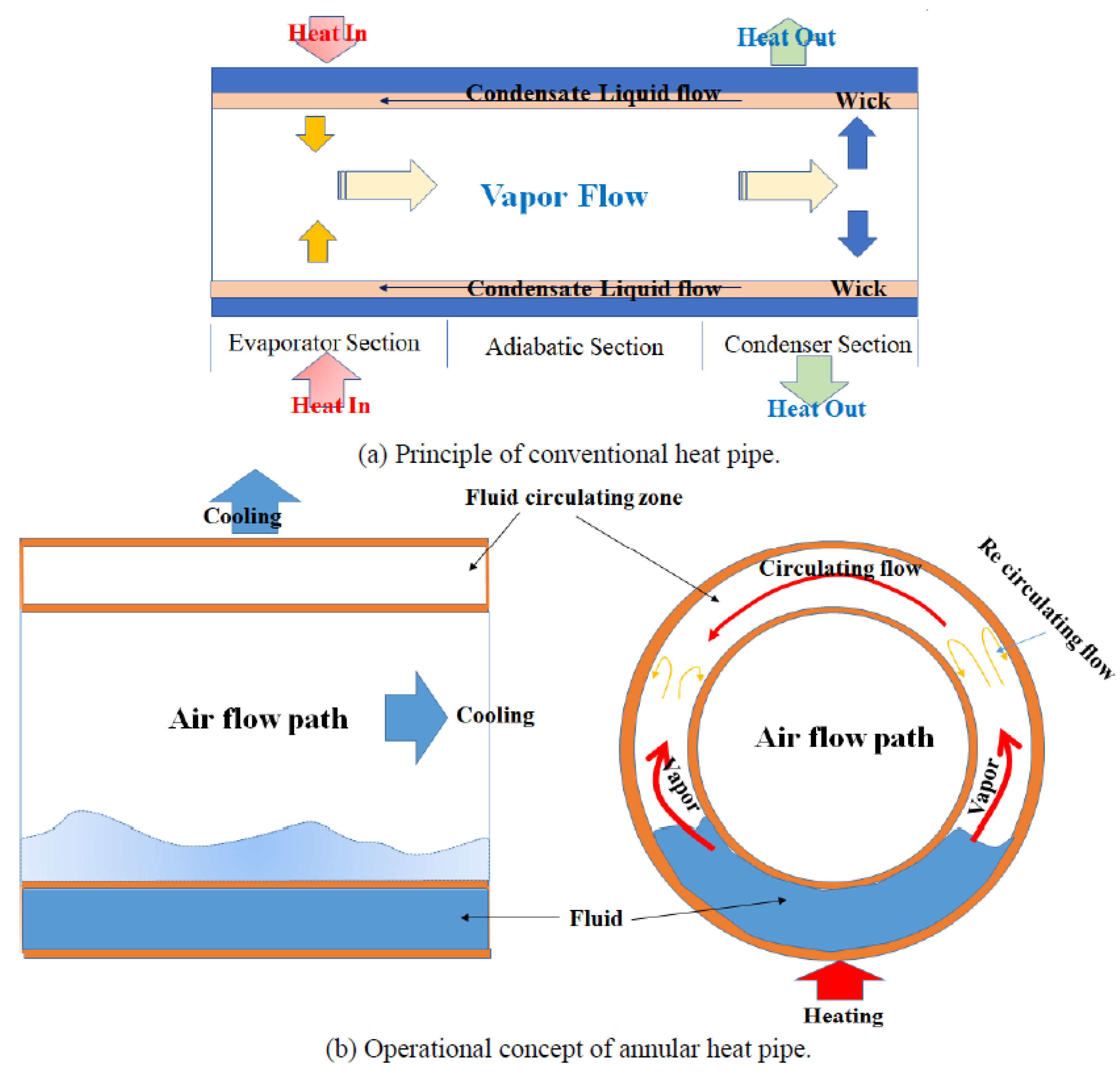
As shown in Figure 1a,b, the concentric annular heat pipe (CHAP, (Figure 1b)) is similar to the conventional heat pipe (CHP) principle (Figure 1a) in which a liquid in contact with the hot interface of a heat pipe absorbs heat from a hot surface and turns into vapor. The vapor then moves along the heat pipe to the cold interface, called the condenser, releases latent heat, and condenses back into liquid. The liquid then returns to the hot interface via capillary action, but the shapes of Figure 1a and Figure 1b are different [5,6]. The liquid circulation process is slightly different from that of a conventional heat pipe, as described in Figure 1b. The annular heat pipe, proposed firstly by Faghri and Thomas in 1989 [7,8], comprises two concentric heat pipes of different diameters. As a large diameter pipe is located on the outside and the small diameter pipe is on the inside, the two ends are sealed. An annular heat pipe has the same shape as Figure 1 and, as the internal space and the external surface are exposed to the outside, the heat transfer area can be significantly increased to increase the heat transfer capacity [9]. In addition, as the area of the room can be expanded without significantly increasing the external diameter, a cooling system with a small and excellent thermal effect can be constructed, if used for the component cooling of an electric vehicle. An annular heat pipe is not only composed of a heat transfer cooling system, but it can also serve as a structure. This allows for the design of cooling flow paths, considering the shape of the annular heat pipe itself, without having to design the flow paths required for cooling separately, thus preventing the loss of materials. An understanding of the flow structure and heat transfer mechanisms is needed, in order to enhance the efficiency of heat transfer for cooling using annular ducts.

The principle of heat pipes was established by Grover in 1964 [5,6], and various forms of heat pipes have been developed with very high heat transfer performance. An annular heat pipe with distilled water as a working fluid showed a 1.85-fold improvement in heat transfer performance, compared to conventional heat pipes, in the experimental results of Faghri and Thomas [7,8]. Faghri found that the performance analysis of these annular heat pipes using the Navier–Stokes equation related to liquid circulating flow is valid. Boo et al. [10] reported experimental results with a copper annular heat pipe (an outer diameter of 25.4 mm, an inner diameter of 11, 8, 6 mm, and a length of 200 mm). Their results showed excellent isothermal properties, and the internal filling rate of the internal working fluid affected performance more.

Various conditions have been used in an annular heat pipe experiment, in which the pipes were constructed of stainless steel (with an outer diameter of 53 mm and an internal diameter of 15.9 mm) by Vijra and Singh [11]. Their experiments, with 50–300 W heating rate applied to annular heat pipes with distilled water and varying angles of 0°, 45°, and 90°, showed that the temperature difference between the evaporator and the condenser was only 3 K, when optimizations were applied.

Yan et al. [12] reported a temperature difference of 15 mK or less in aluminum cells installed inside an annular heat pipe furnace at 657 °C, using sodium as an operating fluid and at temperatures ranging from 500 °C to 1200 °C. Choi et al. [13] built an annular heat pipe by sintering metal nanoparticles. Using the space inside the annular heat pipe as the space of the sintering process, uniform heat distribution was shown and micro-sized porous wicks were produced, sintering them into nanoparticles to demonstrate their functionality. Kammuang-lue et al. [14] studied three concentric thermosyphons of different diameters and found that the annular thermosyphon (ATS) was better adapted to heat transfer applications than the traditional thermosyphon.

Mustafar et al. [15] investigated an annular heat pipe with a condensate center space made of stainless steel tube with an outside diameter of 76.2 mm, an inner diameter of 38.1 mm, and a length of 515 mm. Under experimental conditions, angles from 0 to 90° and internal operating fluid filling ratios from 11 to 43% were studied, with heat of 272 to 302 W. When the internal charged ratio was 11%, optimal isothermal properties were observed and it was shown that the total thermal resistance calculated was 0.08 to 0.31 K/W.

CFD simulation studies of heat pipes have been rarely performed, due to the difficulties of simulating two-phase flow phenomena. Ahmed et al. [16] and Fadhl et al. [17] analyzed and studied the effects of various factors, such as length, wall thickness, heat flux, wick porosity, and wall material, for heat transfer performance estimations of the conventional heat pipe, as shown in Figure 1a, through numerical analysis.

Kapil Dev et al. [18] attempted to simulate a heat pipe by the finite element method. They reported the results in four different cases of heat pipe systems with varying heat flux (560~6400 W/m²) and porosity (0.33~0.74) as influencing parameters. Their Finite element method (FEM) analysis of heat pipe well agreed with experimental results. Temmy et al. [19] presented the results from a vertical heat pipe CFD simulation using the VOF model. A vertical copper tube was used as container material, with an inner diameter of 14.2 mm, a length of 400 mm, and a thickness of 0.9 mm. Cooling by water jackets was adopted for systems with an external diameter of 55 mm. They investigated the effects of using charging ratios of 40, 50, 60, 70, and 100%. The simulation results showed the behavior of both rising hot vapor and falling condensate flowing near the inner wall surface. So, both vapor and condensate flow face each other near the wall. The high momentum phase continues and moves other phases from the wall. Seo et al. [20] presented a simulated flow pattern for the vertical upward flow in a thermosyphon. Their simulated flow patterns showed good agreement with experimental results. They reported that the VOF FEM approach could accurately predict the flow in the thermosyphon. Mroue et al. [21] reported an experimental and numerical investigation of a heat pipe-based heat exchanger. Their experimental results on the heat pipe heat exchanger were compared with a CFD simulation result, where the heat pipe models were solid rods with constant conductivity. Their results showed good agreement within 10% of the experimental values. In their simulation, the heat pipe in their CFD modeling was considered simply as a solid rod with given thermal conductivity, without any consideration on two phase flow inside the heat pipe.

Zhao et al. [22] presented a numerical study on a two-phase closed thermosyphon. Their simulation model was carried out based on the thermal resistance and effective thermal conductivity. They reported that the thermal resistance decreased to a minimum value (0.552 K/W) with increasing heating power, whereas the effective thermal conductivity rose to a maximum (2.07 × 10⁶ W/m∙K). Hussain and Janajreh [23] reported a numerical study of an asymmetrical cylindrical heat pipe. Their analysis showed that the absolute thermal resistance also increased with increasing porosity, due to the decrease in conductivity of the liquid–wick region. They also indicated that the absolute thermal resistance was highest when the evaporator and condenser lengths were equal. Finally, their results showed that the resistance decreased with an increase in internal radius.

Song et al. [24] experimentally studied concentric annular heat pipe heat sink (CAHPHS). They proposed and manufactured the CAHPHS in order to study its thermal performance. CAHPHS is made up of two concentric tubes of different diameters that establish an annular vapor space in a vacuum condition. The most significant benefit of CAHPHS is that it may significantly enhance the area of heat transfer for cooling when compared to existing conventional heat pipes. They worked with stainless steel CAHPHS with diameter ratios of 1.1 and 1.3, inner tube diameters of 76 mm, and lengths of 50 mm. Several experimental factors were tested to assess their effects on the thermal performance of CAHPHS, including 10–70 percent working fluid charged ratio, varied flow rates, flow configurations, and 10–50 W supplied heats. Their experimental results indicated that when water is used as a working fluid and the working fluid filling rate is 10%, the operating characteristics in terms of temperature distribution were best. When methanol is used, thermal characteristics are reported to be better when the filling ratio is 40%. Internal operational characteristics showed that 3-D flows were seen concurrently in axial and circular directions, as well as in circular motion by temperature measurement.

The present work studies the thermo-fluid characteristics of the two-phase flow of an annular heat pipe numerically. CFD analysis of annular heat pipe, with consideration of the liquid–vapor flow region, was performed. A steady CFD analysis was carried out, for the computation of temperature and the prediction of 3D flow characteristics inside the vapor and liquid region, along with surface temperatures at the evaporator and condenser regions. It would be interesting to model the 3D flow region of the heat pipes axially and radially, then calculate the velocity field and the temperature distribution inside. This work analyzes the behavior of the temperature and velocity field inside the annular heat pipe for different heat inputs, different diameter ratios, different filling ratios, and different geometries of the CAHP. This serves to enhance the heat transfer capability of heat pipe applications, by adopting a new heat pipe concept.

2. Numerical Method

Using CFD analysis, the factors affecting the heat transfer performance through comparative consideration with the experimental results obtained in a previous study were determined with thermal flow analysis. The simulation system provides a method for converting the Navier–Stokes equation into several equations and obtaining a solution based on numerical analytical techniques in the dominant equation. We used the FLUENT V17.2 software to carry out numerical analyses under a variety of conditions. The analysis focused on the following conditions and assumptions, in order to compare the simulated and experimentally derived temperatures [24,25]:

-

All phases were assumed to be incompressible flow.

-

The flow of vapor generated was turbulent.

-

The inner vacuum state was 25,041.6 pa, the saturation temperature under the working pressure (operating pressure) was set to 25,041.6 Pa, and the temperature was set to 338.15 K.

-

Conditions other than heating and cooling were insulated conditions, with a heat flux of zero.

-

The heat transfer coefficient was applied in reverse to the value obtained through the thermal flow rate analysis of the 1 m/s conditions. In the inner concentric area, it was 1$6W/m·K$, and in the outer area of the CAHP, it was $5.5W/m·K$ [26].

2.1. Governing Equations and Simulation Model

The governing equations in the simulation involved continuity, mass conservation, and momentum equations based on the Navier–Stokes principle, as follows [25]:

-

Continuity equations:

$$\frac{\partial \mathsf{\rho }}{\partial \mathrm{t}}+\frac{\partial }{\partial {\mathrm{x}}_{\mathrm{i}}}\left({\mathsf{\rho }\mathrm{u}}_{\mathrm{i}}\right)=0$$

(1)

where $\mathsf{\rho }$ is the density of the fluid, $\mathrm{t}\mathrm{is}$ the time, and ${\mathrm{u}}_{\mathrm{i}}$ is the speed of the fluid.

-

Momentum equation:

$$\frac{\partial }{\partial \mathrm{t}}\left({\mathsf{\rho }\mathrm{u}}_{\mathrm{i}}\right)+\frac{\partial }{\partial {\mathrm{x}}_{\mathrm{i}}}\left({\mathsf{\rho }\mathrm{u}}_{\mathrm{i}}{\mathrm{u}}_{\mathrm{j}}\right)=-\frac{\partial \mathrm{p}}{\partial {\mathrm{x}}_{\mathrm{i}}}+\frac{\partial {\mathsf{\tau }}_{\mathrm{ij}}}{\partial {\mathrm{x}}_{\mathrm{j}}}+{\mathrm{g}}_{\mathrm{i}}+{\mathrm{F}}_{\mathrm{i}}+\frac{\partial }{\partial {\mathrm{x}}_{\mathrm{j}}}\left(-\mathsf{\rho }\overline{{\mathrm{u}}_{\mathrm{i}}{}^{\prime }{\mathrm{u}}_{\mathrm{j}}{}^{\prime }}\right)$$

(2)

where p is the pressure, ${\mathsf{\tau }}_{\mathrm{ij}}$ is the shear stress that acts on the fluid, $\rho g_i$ represents the volume force by gravity, and $F_i$ is the external force acting.

$${\mathsf{\tau }}_{\mathrm{ij}}=\left[\mathsf{\mu }\left(\frac{\partial {\mathrm{u}}_{\mathrm{i}}}{\partial {\mathrm{x}}_{\mathrm{j}}}+\frac{\partial {\mathrm{u}}_{\mathrm{j}}}{\partial {\mathrm{x}}_{\mathrm{i}}}\right)\right]-\frac{2}{3}\mathsf{\mu }\frac{\partial {\mathrm{u}}_{\mathrm{k}}}{\partial {\mathrm{x}}_{\mathrm{k}}}{\mathsf{\delta }}_{\mathrm{ij}}$$

(3)

In Equation (3), $\mathsf{\mu }$ represents the viscosity.

-

Energy equation:

$$\frac{\partial }{\partial \mathrm{t}}\left(\mathsf{\rho }\mathrm{E}\right)+\nabla •\left(\mathrm{v}\to \left(\mathsf{\rho }\mathrm{E}+\mathrm{p}\right)\right)=\nabla \left({\mathrm{k}}_{\mathrm{eff}}\nabla \mathrm{T}-{\displaystyle \sum }_{\mathrm{j}}^{}{\mathrm{h}}_{\mathrm{j}}\overrightarrow{{\mathrm{J}}_{\mathrm{j}}}+\left({\overline{\overline{\mathsf{\tau }}}}_{\mathrm{eff}}•\overrightarrow{\mathrm{v}}\right)\right)+{\mathrm{S}}_{\mathrm{h}}$$

(4)

Equation (4) expresses unsteady convection, conduction, and source term. k_eff is the effective thermal conductivity, and the turbulent thermal conductivity is evaluated according to the turbulent model in use. $\overrightarrow{{\mathrm{J}}_{\mathrm{j}}}$ is a diffusion term of the species. Each term of Equation (4) means the transfer of energy due to conduction, diffusion of species, and loss of viscosity from the left. $S_h$ is the source of volumetric heat from the heat and gas generated during a chemical reaction. Enthalpy, h, is defined as Equation (5) for the ideal gas.

$$E=h-\frac{p}{\rho }+\frac{v^2}{2}$$

(5)

If the flow is incompressible, the enthalpy is defined as in Equation (6):

$$h={\displaystyle \sum }_j^{}{Y}_j{h}_j+\frac{p}{\rho }$$

(6)

where $Y_j$ is a mass fraction of species j.

$$h_j={{\displaystyle \int }}_{T_{ref}}^T{c}_{p,j}dT$$

(7)

In Equation (7), $T_{ref}$ is a reference temperature defined as 298.15 K.

A numerical simulation based on the VOF model in ANSYS FLUENT [25] was performed to investigate the condensation process and flow characteristics in an annular heat pipe. Among the multiphase flow approaches in ANSYS FLUENT, the Euler–Euler approach is used for the annular heat pipe flow. This approach was solved by assuming that each phase is a permeable continuum. The VOF method is a model for analyzing two or more immiscible fluids, which can be employed to simulate the evaporation and bubble condensation in two-phase flow. The VOF algorithm is used to calculate the volume fraction of the qth phase through continuity Equation (8), then summing the volume fractions of all phases for one grid. The volume fractions in multiphase flow were described in

Table 1. Volume fraction in multiphase flow.

${\mathbf{\alpha }}_{\mathbf{q}}\left(\mathbf{Volume}\mathbf{Fraction}\right)$	Fluid
0	Empty
1	Full
0 < ${\mathsf{\alpha }}_{\mathrm{q}}$ < 1	one or more other fluids

.

$$\frac{\partial {\alpha }_q}{\partial t}+\nabla •{\alpha }_q\overrightarrow{v_q}=0$$

(8)

$${\displaystyle \sum }_{}^{}{\alpha }_q=1$$

(9)

When using the VOF model for simulating the current annular type heat pipe, the following limitations must be considered:

-

Only a pressure-based solver can be used.

-

All control volumes should be filled with a single fluid phase or a combination of phases.

-

Only one phase can be defined as a compressible (or more) gas.

-

Periodic flow cannot be modeled.

-

Time-stepping equations cannot be used in the implicit VOF exploit scheme in the second order.

The difference in the simulation, due to the constraints of the VOF model, is the vacuum region in the annular heat pipe. In the VOF model, all control volumes must consist of a single fluid phase or a combination of fluid phases. As a result, it is hard to eliminate that a perfect vacuum is generated. However, the current simulation was calculated by applying the Navier–Stokes equation as a basic theory; if the Knudsen number is greater than 1/100, the Navier–Stokes equation is not valid and can be used as a vacuum condition. The definition of Knudsen number is defined in Equation (10), which indicates the number of collisions that occur when a particle passes through a flow region and is assumed to be a continuum if the number of collisions is large enough [27].

$$Kn=\frac{Meanfreepathlength\left(\lambda \right)}{Charateristiclength\left(L_{cha}\right)}$$

(10)

The average free path can be calculated as the average free path of the Boltzmann gas, when applied as follows:

$$Kn=\frac{k_{B}T}{\sqrt{2}\pi d^{2}pL}$$

(11)

where $K_B$ is the Boltzmann constant ($1.380649\times {10}^{-23}$), T is the thermodynamic temperature, d is the diameter of the particles, and p is the total pressure. Knudsen number has the following relationship with the Mach and Reynolds numbers:

$$Kn=\frac{Ma}{Re}\sqrt{\frac{\gamma \pi }{2}}$$

(12)

where Ma is Mach number, Re is Reynolds number, and $\gamma$ is the ratio of specific heat. In the case of the experimental models, the vacuum state was assumed as the Knudson number which was 0.0296 [27].

The k-epsilon turbulence model represents the generation of turbulent kinetic energy (k) and the dissipation rate of turbulence (ε). The realizable k-epsilon model used for the analysis is not a standard model, which assumes isotropy and solves the annular heat pipe using a realizable model which is suitable for an anisotropic curved surface shape:

$$\frac{\partial \left(\rho k\right)}{\partial t}+\nabla ·\left(\rho k\overrightarrow{V}\right)=\nabla ·\left[\left(\mu +\frac{{\mu }_t}{{\sigma }_k}\right)\nabla k\right]+G_b+G_k-\rho \epsilon +S_k$$

(13)

$$\frac{\partial \left(\rho \epsilon \right)}{\partial t}+\nabla ·\left(\rho \epsilon \overrightarrow{V}\right)=\nabla ·\left[\left(\mu +\frac{{\mu }_t}{{\sigma }_k}\right)\nabla \mathsf{\epsilon }\right]+C_{1\epsilon }\frac{\epsilon }{k}\left(G_k+C_{3\epsilon }{G}_b\right)-C_{2\epsilon }\rho \frac{{\epsilon }^2}{k}+S_{\epsilon }$$

(14)

where ${\mu }_t$ is the mixture phase turbulent viscosity; $G_k$ and $G_b$ are the generations of turbulence kinetic energy owing to mean velocities and buoyancy respectively; $S_k$ and $S_{\epsilon }$ are additional source terms. The constants in Equation (14) are given as, $C_{\mu }=0.09,C_{1,\epsilon }=1.44,C_{2.\epsilon }=1.92,{\sigma }_k=1.0,{\sigma }_{\epsilon }=1.3$ [25].

2.2. Evaporation–Condensation Model

In case of the phase change model, the magnitude of the liquid flow must be confirmed by experimentation, and it is necessary to know the mass transfer coefficient between phases. Therefore, in the present simulation, the Lee model [28] in Equation (15) was used as the phase change model, where the gas transfer equation of Equation (11) controls the liquid–vapor mass transfer (evaporation and condensation) process:

$$\frac{\partial }{\partial t}\left({\alpha }_v{\rho }_v\right)+\nabla ·\left({\alpha }_v{\rho }_v\stackrel{\rightharpoonup }{V_v}\right)=\dot{m_{lv}}-\dot{m_{vl}}$$

(15)

In Equation (15), α_v, ρ_v, $\stackrel{\rightharpoonup }{V_v}$ represent the volume fraction, the density, and the velocity of the gas phase, respectively. ${\dot{m}}_{l\to v}$ and ${\dot{m}}_{v\to l}$ express the mass transfer rate of evaporation and condensation, respectively. Furthermore, forward mass transfer is defined as the evaporation-condensation process from liquid to vapor. Based on different temperatures, the mass transfer model can be described in

Table 2. Mass transfer model by Lee [29].

Phase Change	Temperature	Phase	Mass Transfer
Evaporation	${\mathrm{T}}_{\mathrm{l}}>{\mathrm{T}}_{\mathrm{sat}}$	Liquid	${\dot{\mathrm{m}}}_{\mathrm{l}\to \mathrm{v}}=-0.1{\ast \mathsf{\alpha }}_{\mathrm{l}}{\mathsf{\rho }}_{\mathrm{l}}\frac{\left({\mathrm{T}}_{\mathrm{l}}-{\mathrm{T}}_{\mathrm{sat}}\right)}{{\mathrm{T}}_{\mathrm{sat}}}$
		Vapor	${\dot{\mathrm{m}}}_{\mathrm{l}\to \mathrm{v}}=0.1{\ast \mathsf{\alpha }}_{\mathrm{l}}{\mathsf{\rho }}_{\mathrm{l}}\frac{\left({\mathrm{T}}_{\mathrm{l}}-{\mathrm{T}}_{\mathrm{sat}}\right)}{{\mathrm{T}}_{\mathrm{sat}}}$
Condensation	${\mathrm{T}}_{\mathrm{v}}<{\mathrm{T}}_{\mathrm{sat}}$	Liquid	${\dot{\mathrm{m}}}_{\mathrm{v}\to \mathrm{l}}=0.1{\ast \mathsf{\alpha }}_{\mathrm{v}}{\mathsf{\rho }}_{\mathrm{v}}\frac{\left({\mathrm{T}}_{\mathrm{sat}}-{\mathrm{T}}_{\mathrm{v}}\right)}{{\mathrm{T}}_{\mathrm{sat}}}$
		Vapor	${\dot{\mathrm{m}}}_{\mathrm{v}\to \mathrm{l}}=-0.1{\ast \mathsf{\alpha }}_{\mathrm{v}}{\mathsf{\rho }}_{\mathrm{v}}\frac{\left({\mathrm{T}}_{\mathrm{sat}}-{\mathrm{T}}_{\mathrm{v}}\right)}{{\mathrm{T}}_{\mathrm{sat}}}$

[29].

In Lee model, liquid evaporates when the temperature is higher than the saturation temperature of each working fluid. The mass transfer rate multiplied by the latent heat yields the source term in the energy equation. The Hertz–Knudsen equation as Equation (16) is generally used to predict evaporation/condensation rate, $\dot{m}$. It indicates that the rate of evaporation/condensation is proportional to the difference in system pressure and equilibrium pressure for liquid/vapor coexistence [28,30]:

$$\dot{m}=\mathsf{\beta }\sqrt{\frac{\mathrm{M}}{2{\mathsf{\pi }\mathrm{RT}}_{\mathrm{sat}}}}\left({\mathrm{P}}^{\ast }-{\mathrm{P}}_{\mathrm{sat}}\right)$$

(16)

where P is the pressure, $P^{\ast }$ is the partial pressure of the vapor, T is the temperature, R means the gas constant, and $\mathsf{\beta }$ is the absorption coefficient, which represents the vapor molecules that are absorbed by the liquid surface.

Clapeyron–Clausius equation (Equation (17)) represents the relationship between the saturation temperature and the pressure and can be used to obtain the temperature change from the pressure change close to the saturation condition [25]:

$$\frac{dP}{dT}=\frac{L}{T\left(v_v-v_l\right)}$$

(17)

The continuous surface force model for surface tension is determined by modifying the surface force acting on the liquid–gas interface, using the following equations for the volume force produced using Gaussian divergence clearance applied to the external force element of the momentum preservation equation:

$$p_2-p_1=\sigma \left(\frac{1}{R_1}+\frac{1}{R_2}\right)$$

(18)

where $p_1\mathrm{and} p_2$ are the pressures on both sides of the surface, $R_1 \mathrm{and} R_2$ are the curvatures, $\mathsf{\rho }$ is the average density for the volume, and $\mathsf{\sigma }$ is the surface tension. As expressed in Equation (19), the surface tension between water and vapor is applied using the equation in the two-phase flow thermosyphon analysis of Fadhl [17]:

$$\mathsf{\sigma }=0.09805856-1.845\ast {10}^{-5}\ast \mathrm{T}-2.3\ast {10}^{-7}{\ast \mathrm{T}}^2$$

(19)

2.3. 2D and 3D Numerical Models and Validation

The simulation model for the analysis of flow characteristics, performance comparison with conventional heat pipes, and flow characteristics by the internal width was conducted under four conditions. The basic model of the CAHP to be simulated is shown in Figure 2. The current numerical models are divided into 2D geometrical simulation assuming symmetry and a 3D model simulated using the same models used in previous experimental work [24]. The 2D numerical model has a faster analysis time than the 3D model, making it easy to determine the tendency of various conditions. However, with the 2D model, it is difficult to determine the flow of the axial direction. Therefore, the 2D simulation was carried out and validated by comparison with the experimental results for the external conditions, and the simulation validity was verified. Then, the effects of various parameters were predicted, in order to identify the tendency of change of the factors affecting the thermal performance of the CAHP.

2.3.1. Two-Dimensional CFD Model (2D Model)

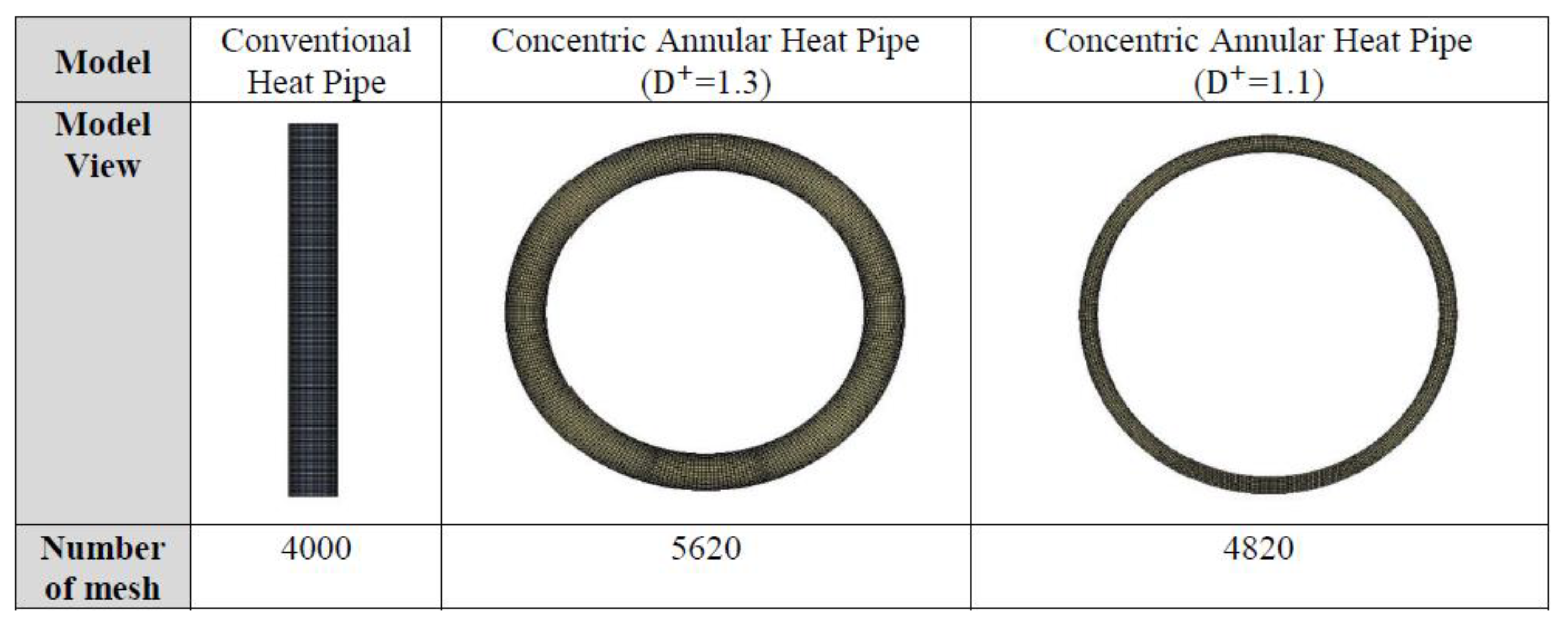
The presented 2D simulation model had an outer diameter of 98 mm, inner diameter of 78 mm in the shape of D⁺ = 1.3, and the wall thickness of 1 mm. The container material was set as steel, which is the same as the experimental system [24]. The thermal resistance of the wall condition is given as

$$R=\frac{t}{k\ast A}$$

(20)

where R is the thermal resistance of the solid material, t is the wall thickness, k is the thermal conductivity of the solid material, and A is the area. The basic geometry of the analytical model is shown in Figure 3.

By configuring the evaporator and condenser positions similarly to the conventional heat pipe, the 2D simulation was designed for the CAHP (Concentric annular heat pipe). The heat transfer performance of the asymmetrical CAHP was verified by a comparative simulation study between the symmetric and asymmetric shapes. As shown in Figure 4, the conventional simple heat pipe (Figure 4a) and the CAHP shape (Figure 4b) were set to compare the thermal performance with the same length configuration for the evaporation and condensation sections.

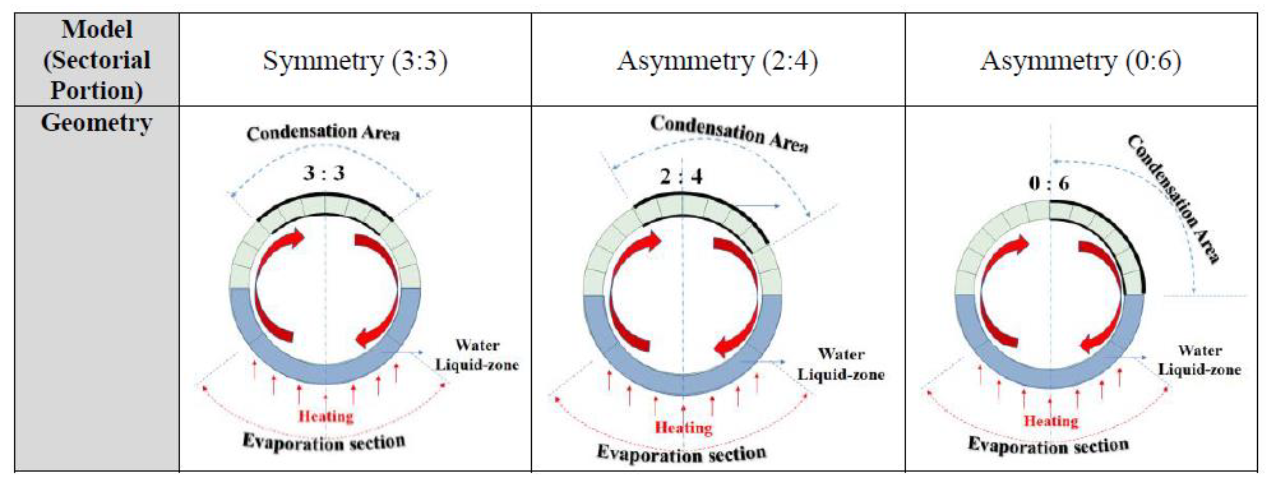
In the model, 20 mm of the bottom was heated in the evaporation section and condensed in the condensation section (20 mm at the upper section) through the adiabatic transport section in the middle. The working fluid (water) occupied 50% of the total volume and the remaining 50% volume was configured as ambient. As shown in Figure 4b, the CAHP model for simulation was divided into 12 divisions with 15° angular distance. As shown in Figure 5, the CAHP model was configured as a condensation section for both the inside and outside, in order to fit each ratio. Through three cases, symmetric and asymmetric effects in the CAHP were simulated.

2.3.2. Three-Dimensional Model (3D Model)

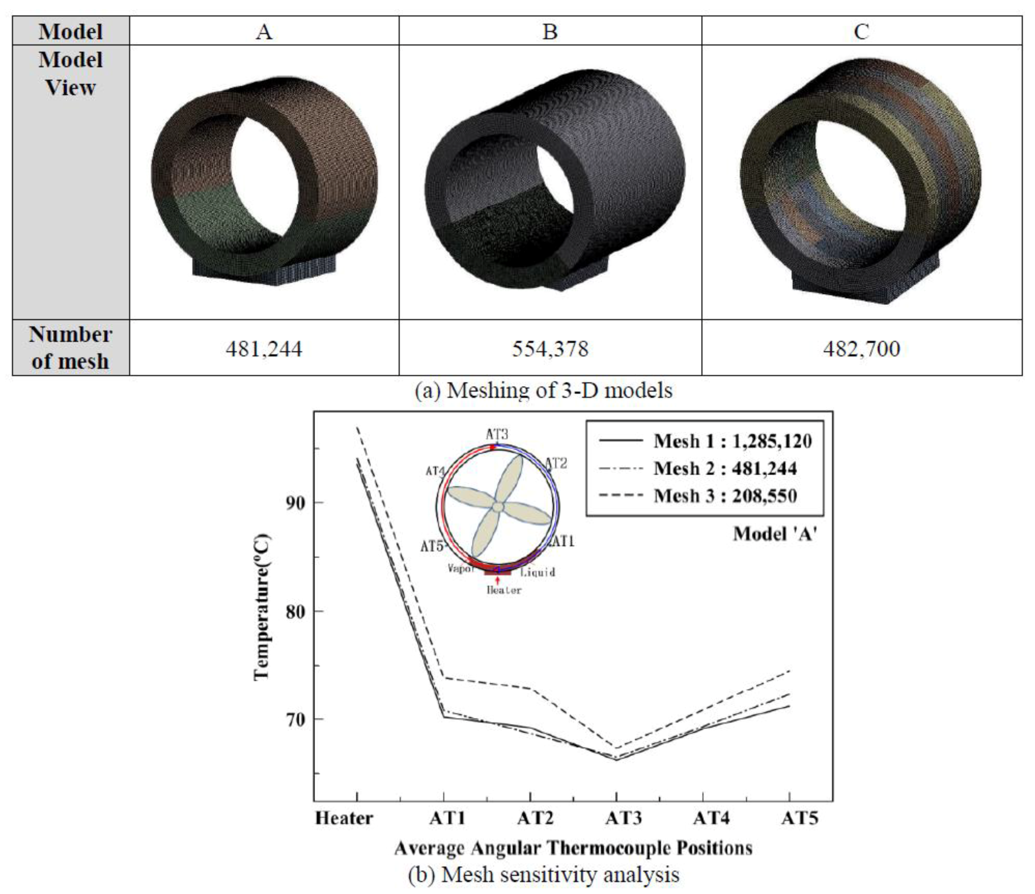
In the three-dimensional analysis, the flow in the axial direction was modeled simultaneously with 2D analysis. In the 3D models, the walls were modeled directly, constructing cell zones with steel (solid). It was configured as shown in Figure 6. As shown in Figure 6, three types of 3D shapes—50 and 100 mm long models and a 50 mm sectorial model—were prepared to simulate a CAHP, labeled Models ‘A’, ‘B’ and ‘C’, respectively.

Figure 7 shows a detailed geometrical view of the 3D sectorial Model ‘C’ of Figure 6. The condenser surface area of Model ‘C’ was increased with 10 mm step (5 divisions) and an angular step of 60°. The condensation area increased axially from flow inlet to outlet. Total area of the CAHP with varied condenser area shown in Figure 7 was 2.384 × 10⁻³ m².

The model shown in Figure 7 was used to investigate asymmetric condensation in the axial and radial direction. In model ‘C’, the area of the condenser section, compared to the conventional symmetrical model ‘A’, is reduced to 36.7%.

2.4. Grid Configuration and Mesh Generation

In any numerical study, a grid independence or mesh sensitivity analysis should be carried out, in order to ensure that the results obtained from the simulation work are sufficiently accurate. Figure 8 and Figure 9a,b show the 2D and 3D mesh shapes and sensitivity analysis according to the mesh conditions. The orthogonal quality and the skewness of the isotropy for the orthogonality of the mesh were examined. These two characteristics of the mesh in CFD analysis greatly affect the analysis results. In general, the quality of the orthogonality was between 0.15 and 0.95, and the quality of the isotropy indicated that we could proceed with the simulation. In the current pre-grid test, the quality value of the 2D case was over 0.1 for the isotropy and 0.9 for the orthogonality. For the 3D simulation, the maximum values of isotropy quality were 0.65168 (A case), 0.79927 (B case), and 0.68549 (C case). The minimum values of orthogonality were 0.53687, 0.23313, and 0.49214, respectively [29].

Furthermore, in order to improve the accuracy of CFD simulation and reduce computing costs, grid dependence tests were conducted by creating three distinct meshes with coarse, medium, and fine grids to examine how mesh quality influences CFD simulation results. To validate the grid sensitivity analysis, Model ‘A’ of Figure 9a is modeled in various mesh sizes, as illustrated in Figure 9b (Mesh 1: 1,285,120 nodes, Mesh 2: 481,244 nodes and Mesh 3: 208,550 nodes). Figure 9b shows the result of the calculations. Updating the mesh illustrates that the solution is grid independent. As a result, we choose Mesh 2 (481,244 nodes) to prevent high calculation times and solution instability.

2.5. Boundary Conditions

The initial boundary conditions for the current simulation are given in

Table 3. Boundary conditions.

Initial Conditions	Value
Initial Temperature	298.15 K
Operating pressure	0.31202 bar
Saturation temperature	343.15 K
Heating power	30,000 $\mathrm{W}/{\mathrm{m}}^2$
Heat transfer coefficient (Inner concentric space, forced convection)	16 W/m2·K
Heat transfer coefficient (Outer surface, natural convection)	5.5 W/m2·K
Free stream temperature	298.15 K

. Assuming a surface with a constant surface heat flow rate of the heating section, the Neumann boundary conditions were applied as follows [29]. Surface heat transfer coefficient values, calculated inversely through the analysis of the same model as that for the forced convection and natural convection conditions of Table 3, were applied.

3. Numerical Analysis and Results

A numerical study should be compared with experimental results, in order to verify its reliability. For the current simulation study, the simulation results were validated using the results of a previous experimental study by Song et al. [24].

3.1. Effect on Working Fluid Filling Ratio

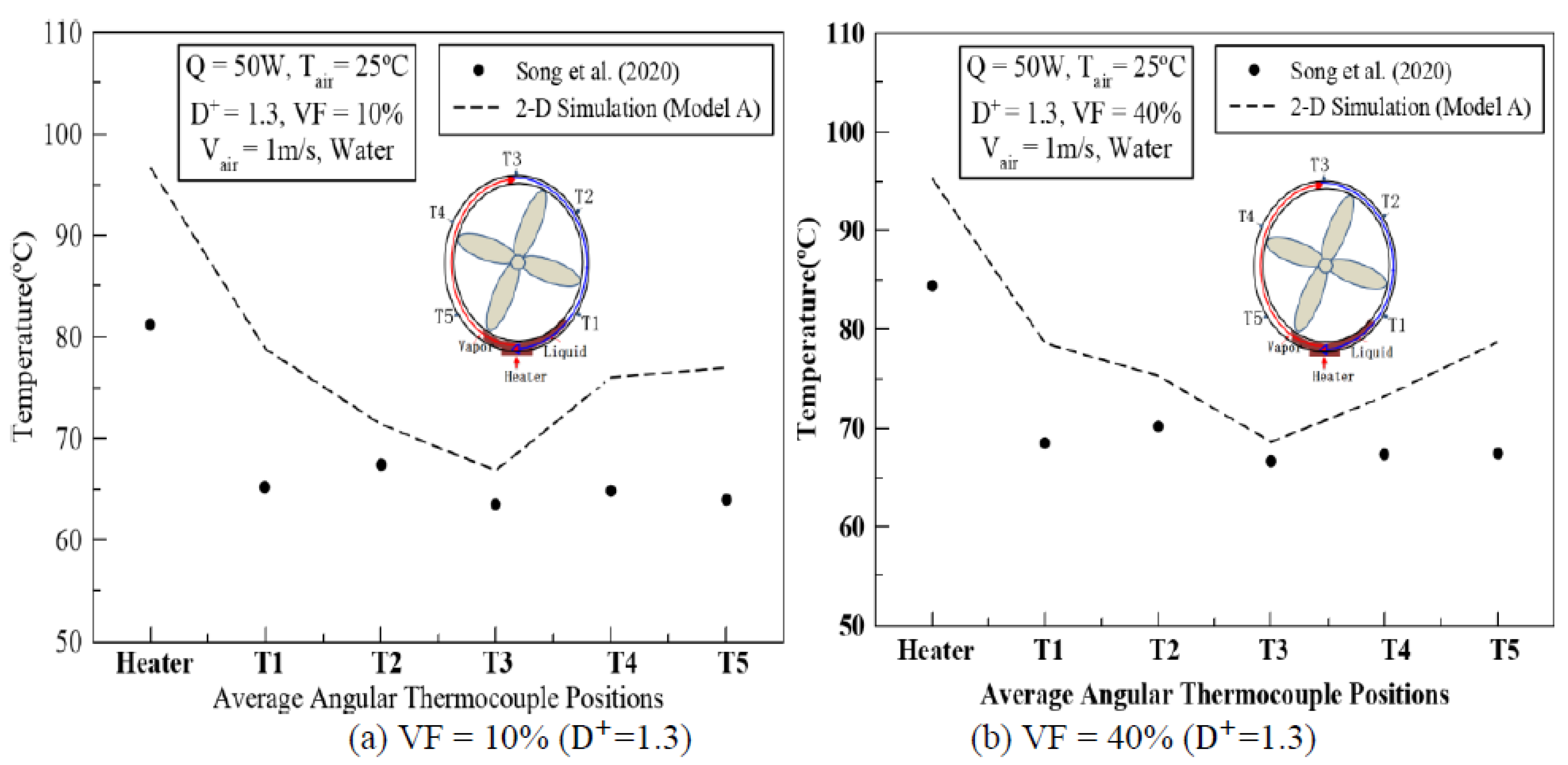
The effect of the working fluid volume ratio was simulated using VF = 10% and 40%. The simulation results were compared to the experimental values. As shown in Figure 10a,b, the experimental results showed a lower temperature distribution when VF = 10%. Comparison between simulation and experimental results revealed a slightly larger temperature difference when VF = 10% than when VF = 40%. Furthermore, the maximum temperature deviation was 15.4 °C for VF = 10% and 10.83 °C for 40% in the heater. The minimum deviation was 3.24 °C for 10% and 1.95 °C for 40%, more closely matching the experimental value. The reason for this was that, when VF = 10%, it would have been difficult to properly simulate the internal working fluid circulation, due to the low internal liquid volume.

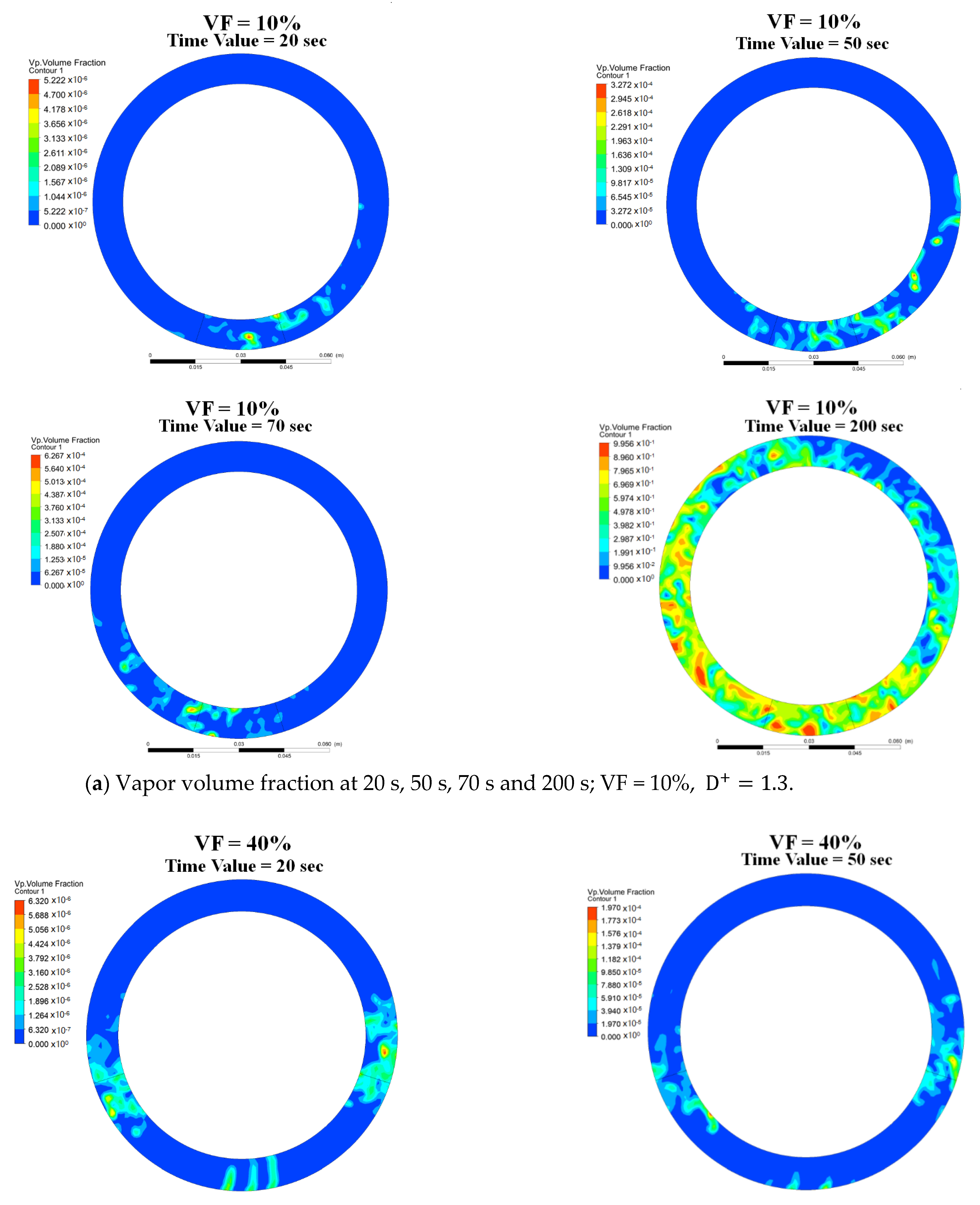
As shown in Figure 11a,b, when the given variables were D⁺ = 1.3 and VF = 10%, the flow of vapor was found to move from side to side over time. In the CAHP with D⁺ = 1.3 and VF = 40%, the flow of vapor was distributed from side to side over time, then determining the direction of movement back to the left. Finally, after 200 s, the evaporation process was activated at the evaporation section and the flow direction was determined to one side; it was confirmed that it flows and condenses at the upper condenser section and returns to the evaporator section. Figure 11 shows the simulation results over time. In this figure, we can see that vapor started to develop inside the CAHP when the time reached 20, 50, 70, and 200 s, and the vapor flowed to the left or right. Figure 11a,b show that, at VF = 10%, it flowed from right to left while, at VF = 40%, it vibrated from side to side. It can be confirmed that the larger the amount of working fluid, the harder it is to overcome the pressure difference between the evaporator and the condenser.

3.2. Effect of Different Diameter Ratio (D⁺)

Figure 12a presents the effect of the diameter ratio in the 2D analysis and also shows the temperature distribution at each location of the annular tube, according to the diameter ratio of the two pipes. In the two-dimensional analysis, the temperature distribution was lower than in the case of D⁺ = 1.1; thus, the vapor volume fraction of the operating fluid was determined, in order to determine the reason. Unlike the case of D⁺ = 1.3 in Figure 11b, in the case of D⁺ = 1.1, the internal fluid circulated according to the pressure difference between the top and bottom due to the vapor pressure generated by the evaporator, where the temperature of the evaporator that was not in contact with the liquid increased. This was induced from the liquid deficiency region, due to the low vapor volume fraction. This phenomenon is due to a large amount of small vapor bubble flow passage forming a locally liquid deficient region. At this moment, specifically, the liquid-deficient evaporator can exist. As shown in Figure 12b, a locally high liquid volume fraction was observed.

3.3. Effects of Symmetry and Asymmetry

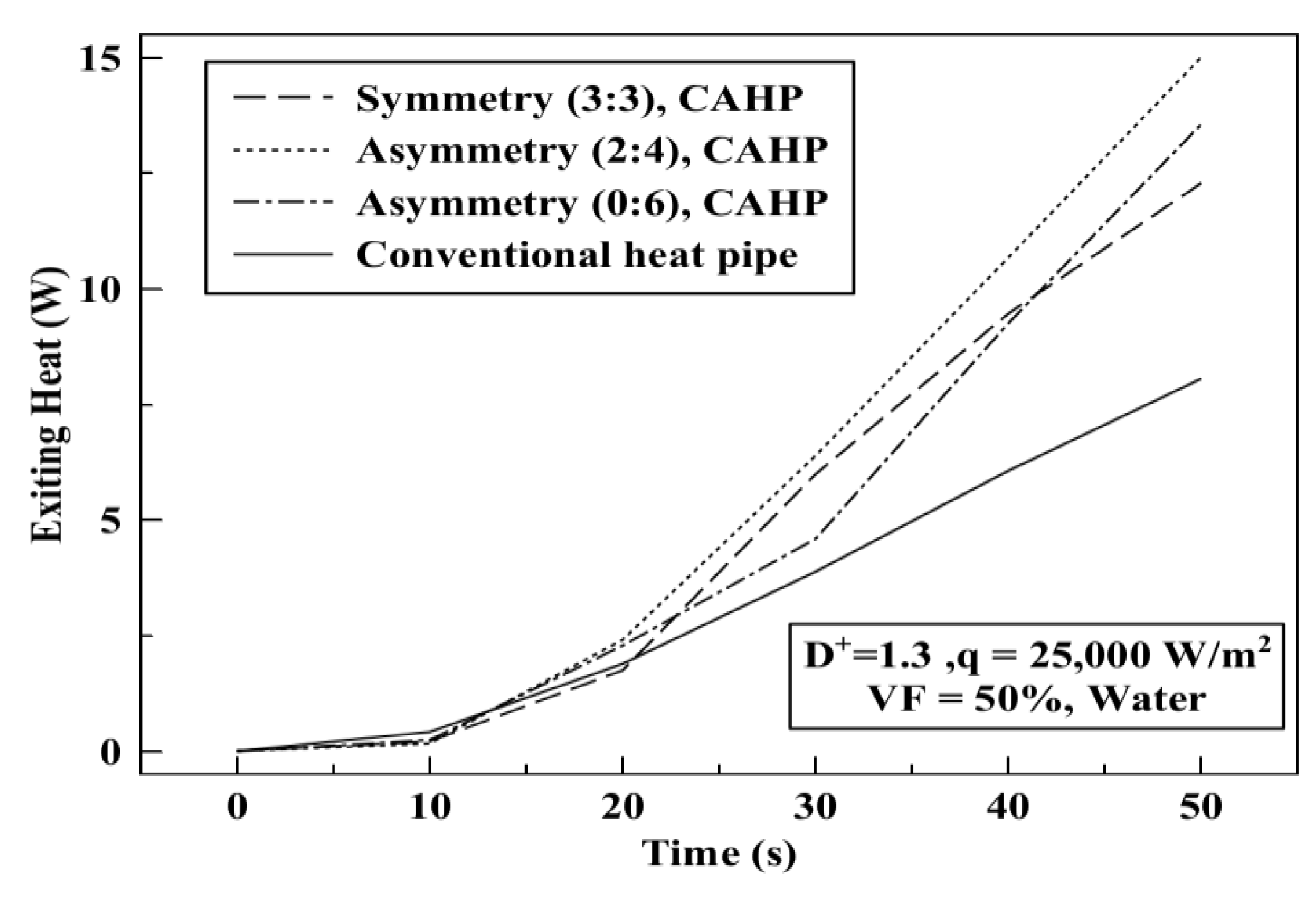
In Figure 13 and

Table 4. Temperature in each condition.

Type	Max Temperature (°C)
CAHP—Symmetry (3:3)	76.3
CAHP—Asymmetry (2:4)	65.4
CAHP—Asymmetry (0:6)	70.7
Conventional heat pipe	78.2

, an analysis to determine the effects of symmetry and asymmetry on the heat transfer performance, compared to conventional heat pipes, on the condenser section of the 2D model was carried out. In the case of conventional heat pipes, there are no difficulties in comparing the results proceeded by 2D simulation, as the heat-transfer method is just a simple circulation process and, so, the two-dimensional method can be applied to the current simulation. Figure 13 shows the heat transfer performance according to each condition, while Table 4 gives the maximum temperature at 50 s of simulation time. This means that the unequal pressure distribution in circular geometry can drive the liquid circular motion as a driving force. As shown in Figure 13, the CAHP showed much higher thermal performance, compared to the conventional heat pipe (over 1.8 times); similar to the results of Fhagri and Thomas [8].

As a result of the analysis, when comparing the symmetric and asymmetric conditions that divide the two sides of the condensation section, the amount of heat removed in case of asymmetric (2:4) was 33.5% higher than that due to symmetry (3:3). In addition, when comparing a conventional heat pipe with annular heat pipes with asymmetry (2:4), the transferred heat was 52.5% higher. This analysis first indicates that annular heat pipes are more effective in heat dissipation than conventional heat pipes. Next, the effect was better when the condenser of the annular heat pipe was asymmetric than when it was symmetric, indicating the effect of inducing flow by setting the condenser asymmetrically. Asymmetry of 2:4, compared to 0:6 asymmetry, led to 10.6% more heat removal.

3.4. Axial Flow Effects through 3D Modeling

Modeling to determine the axial flow effect was conducted for 200 s using the initial conditions described in

Table 5. Velocity component and temperature under each condition.

Variable Components	A (50 mm)	B (100 mm)	C (50 mm, Asymmetry)
Velocity U (m/s)	1.638~−0.729	0.651~−0.497	1.943~−1.828
Velocity V (m/s)	1.388~−1.148	0.843~−0.645	1.597~−2.609
Velocity W (m/s)	0.704~−1.191	0.857~−1.286	2.282~−2.340
Max Temperature (°C)	94.172	86.97	91.85

. The time step proceeded by 0.0005 s for the 50 mm and 100 mm 3D model analyses of CAHP with ${\mathrm{D}}^{+}$ = 1.3 and VF = 40%. The temperature at the heater position in the 2D and 3D models was similar, as heat transfer through the flow of the circumference, rather than in the axial direction, is dominant when ${\mathrm{D}}^{+}$ = 1.3 and VF = 40%. The distribution of velocity by direction in the models could be determined.

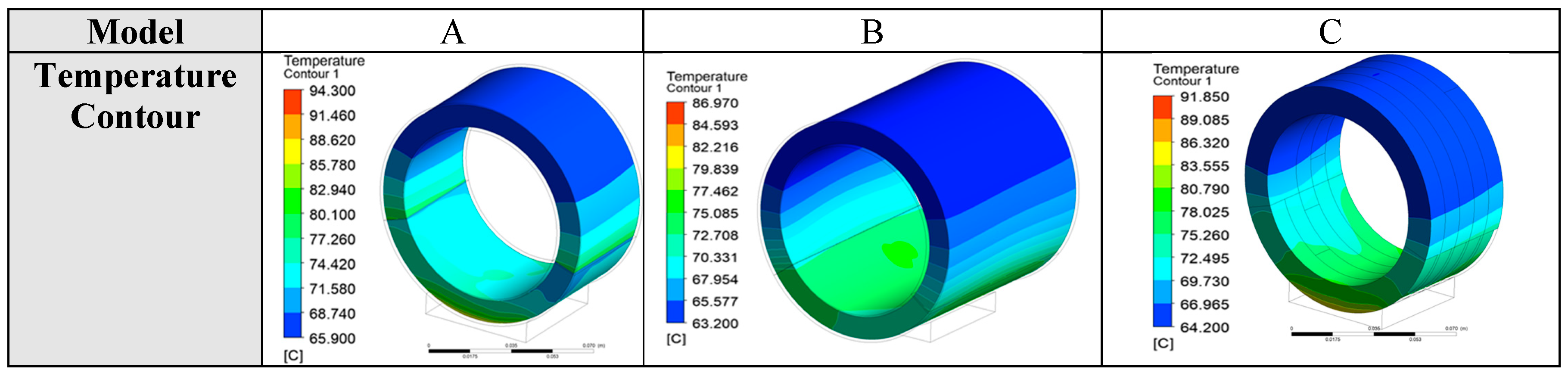
In Table 5, velocity, U is a horizontal direction component, velocity V is a vertical direction component, and velocity W is an axial component. In the case of Model ‘A’, the velocity distributions for the horizontal, vertical, and axial directions were similar, and it was possible to investigate the three-dimensional flow behavior. In model ‘B’, it can be seen that the speed in the axial direction was a little larger. Model ‘C’ had a large velocity distribution in all directions, indicating an active flow. In addition, the velocity distribution in the axial direction appeared to be larger than other components. This difference in flow generated the temperature difference between the three models. Axial flow occurs when asymmetric flow from the center is induced. Due to this difference, the 100 mm annular heat pipe showed a lower temperature distribution than the 50 mm CAHP. The temperature contour is presented for the three models in Figure 14; the highest temperature was 94.172 °C for symmetric model ‘A’ and 86.97 °C for model ‘B’, with a length direction of 100 mm. In the case of model ‘B’, the heat transfer area was twice as large, compared to model ‘A’. For the 50 mm model ‘C’, consisting of axial asymmetric cooling surfaces, the heater temperature was 2.32 °C lower than the 50 mm model ‘A’, which cools the entire center. This induces axial flow, resulting in isolated vapor flow due to internal circulation, indicating improved heat transfer performance.

3.5. Volume Fraction of Vapor and Streamline Analysis

As shown in Equation (21), the flow streamline is defined as follows, in the same line as the direction of the tangent velocity vector on each point:

$$V\times dr=0$$

(21)

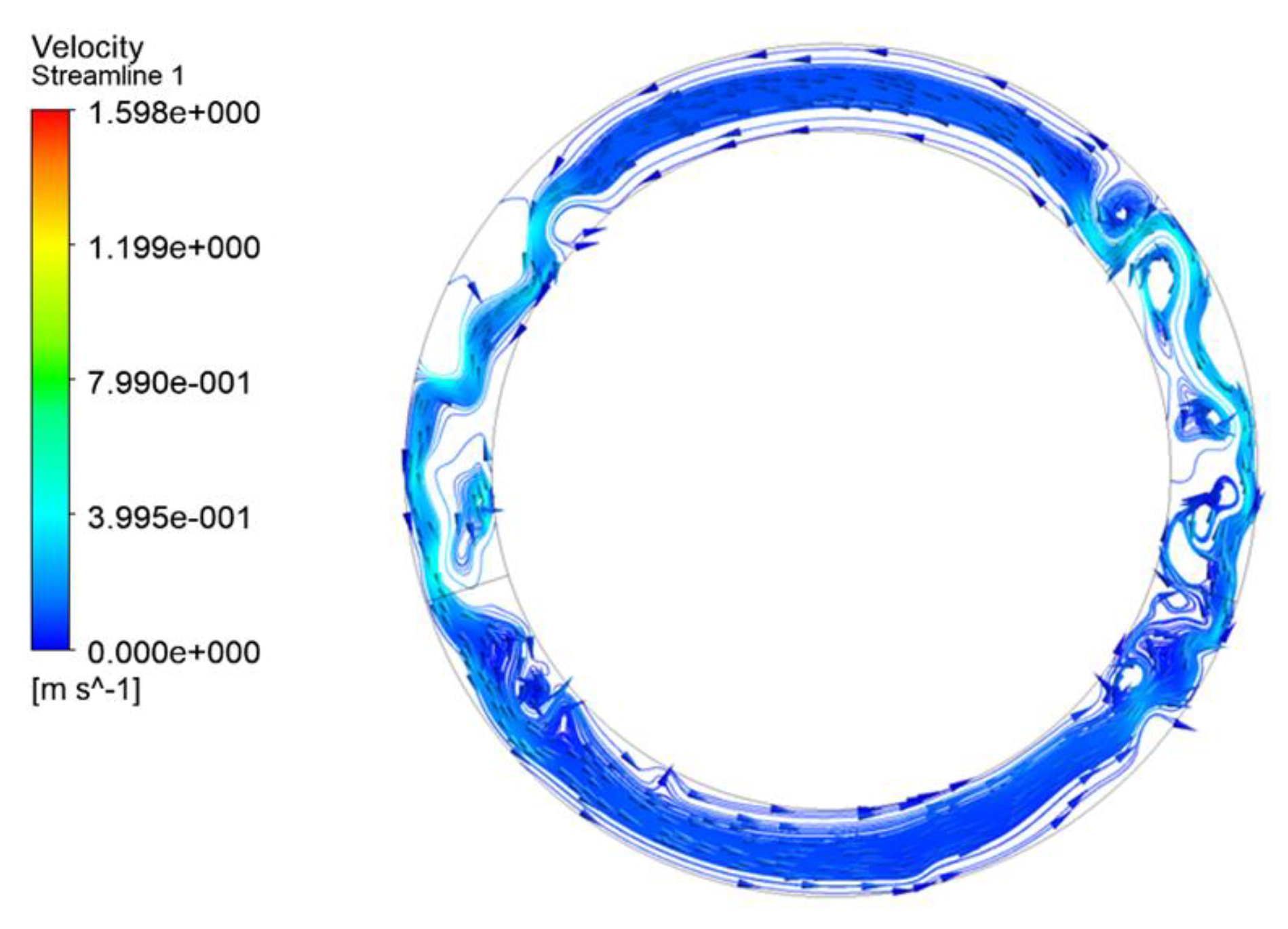
It is difficult to express the path-line of the fluid-specific particles with the VOF model, as it represents the ratio that each fluid contains per cell, rather than representing each particle. Therefore, the current simulation could check the flow direction through the streamline. As shown in Figure 15, the streamline results when the internal filling rates of the CAHP were 40% and 10% also appeared similar. In case of a contour that appears in the 2D simulation at 200 s, it can be observed that the flow has a clockwise circulating motion.

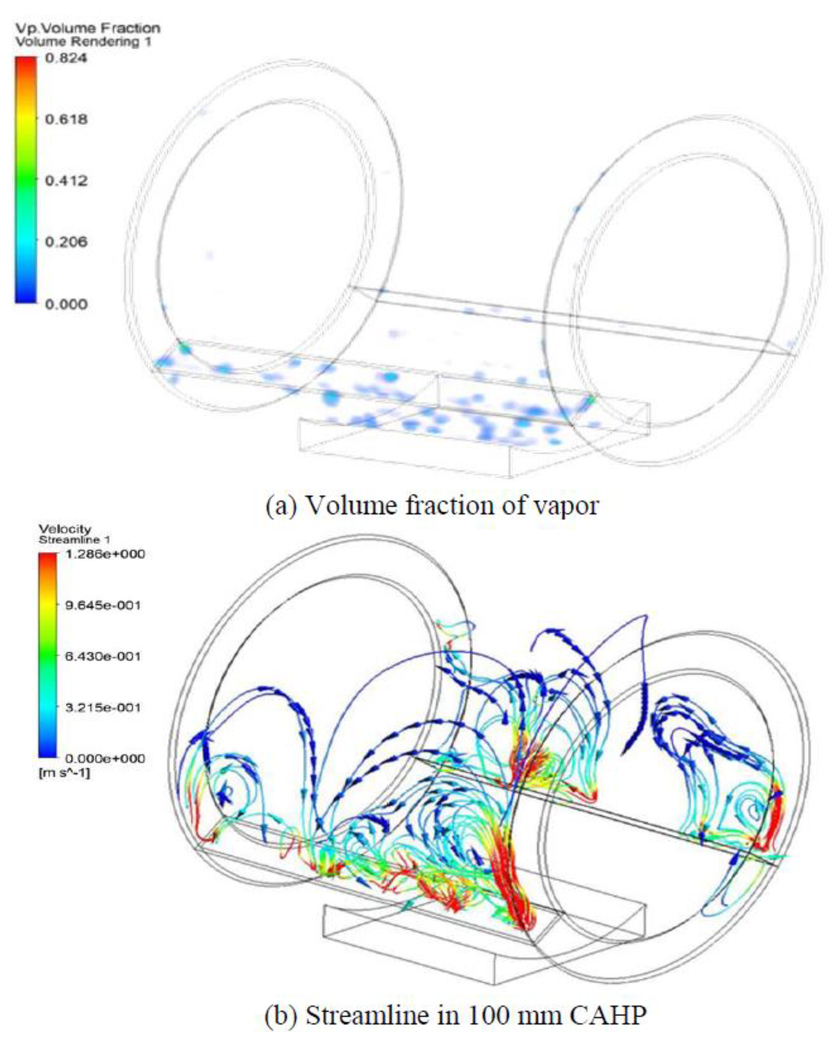
Figure 16a,b show the result of the 3D simulation at 200 s for Model ‘A’. As shown in Figure 16, the vapor evaporated from the surface of the water moved along the CAHP in both radial and axial directions. Figure 16a shows the vapor formation in the evaporator section. In addition, as shown in Figure 16b, due to the center cooling, some of the vapor rising to the top end was unable to reach the end, resulting in condensing phenomena, which was guessed as recirculation flow locally. As a result, the internal fluid oscillated from side to side, showing a phenomenon that circulated intermittently. In addition, the flow behavior in the irregular axial direction was also observed, as was confirmed in the experiment [24].

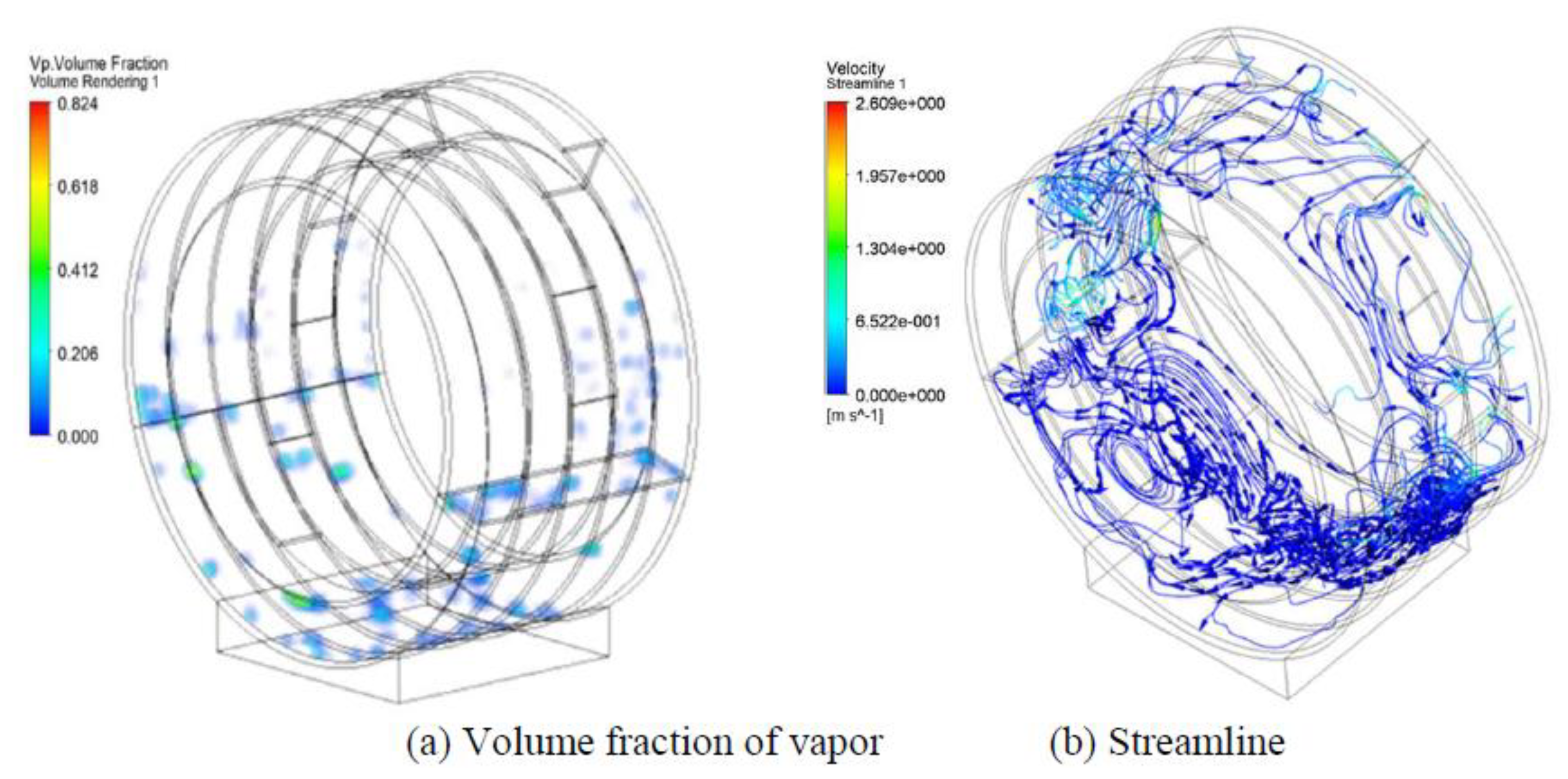
Figure 17a,b show the vapor volume fraction and streamline of the 3D simulation at 200 s for Model ‘B’. In Figure 17a, the vapor from the surface of the water is evaporated. On both sides, flow resistance occurs due to evaporation; however, at the center, the flow shows that the vapor is condensed inwards without resistance. The overall temperature distribution at the surface was low. Therefore, the evaporated vapor was rapidly condensed.

Figure 18 shows the result of the 3D simulation in the calculation of Model ‘C’, with tapered sectorial area structure of the condenser, as shown in Figure 7. As it can be seen from Figure 18a,b, the left portion of CAHP was cooled entirely; the more to the right, the smaller the cooling area, according to the tapered sectorial structure. The vapor also moved towards the rear of the axial direction due to temperature differences, and condensate was observed to flow down to the front of the axial direction. In the case of the sectorial Model ‘C’, the temperature of the heater part was lower than that in the symmetric Model ‘A’. This can be attributed to the active cooling activity through the axial flow. Figure 18 shows a comparison of results between the experiment [24] and simulation.

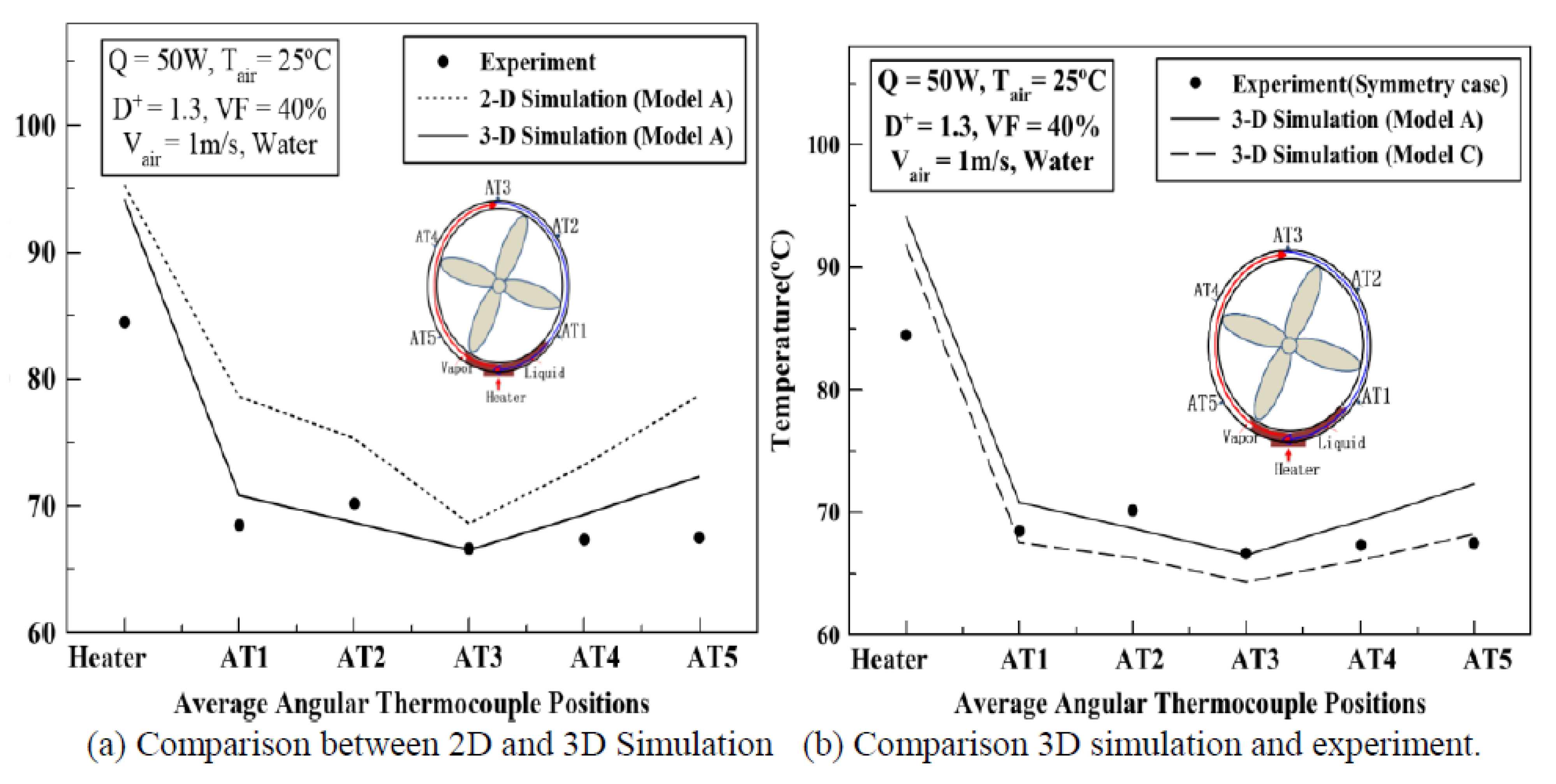
Figure 19a,b present the validated simulation results for 2D and 3D models. As shown in Figure 19a, the 3D simulation showed much better agreement with the experimental results. This was because the axial flow in the 2D simulation was overestimated, in terms of heat transfer performance, and the 2D simulation cannot show the effect of axial flow characteristics. In model ‘A’, the 50 mm length system does not effectively and actively capture the circulatory behavior. Furthermore, as shown in Figure 19b, the experimental result showed the trend of the temperature profile of the asymmetric case. This means that the experimental system cannot have exactly symmetric structure. As shown in Figure 19b, 3-D simulation shows very promised agreement with experimental results. This means that the axial flow has been highly influenced by the thermal performance.

4. Conclusions

The following are the results of our parametric simulation study to improve the heat transfer performance of annular heat pipes:

• The temperature difference between the experimental results and the simulation with various CAHP charge ratios was proven to be less than 15.4 °C. The main difference between 2-D and 3-D simulations was induced from the CAHP structure. There was no axial flow in the 2-D simulation; nevertheless, there was an axial flow in the real experiments, and its influence resulted in a temperature difference between 10% and 40% of VF when compared to that reported in the experiment.
• Furthermore, with given high heat flux through simulation, dry-out occurred inside an annular heat pipe with VF = 10%.
• The diameter ratio was the most important factor in CAHP thermal performance. When the diameter ratio is reduced from D⁺ = 1.3 to D⁺ = 1.1, the liquid deficiency effect becomes severe. In a 2-D simulation, large vapor bubbles with VF = 10 percent induce local liquid absence zones and temperature rises.
• The heat transfer rate of asymmetric annular heat pipes was 52.5 percent greater than that of conventional heat pipes as a result of the 2D simulation, and the efficiency was 10.6 percent greater than that of the symmetric condenser CAHP. This indicates that by managing the flow in the circumferential direction, the asymmetric structure may increase heat transfer performance.
• The 3D simulation agrees with the experimental results to a reasonable degree. This indicates that thermal performance has had a substantial influence on axial flow.

References

- IEA. World Energy Outlook; IEA OECD: Paris, France, 2020. [Google Scholar]
- Zhang, X.; Kong, X.; Li, G.; Li, J. Thermodynamic assessment of active cooling/heating methods for lithium-ion batteries of electric vehicles in extreme conditions. Energy 2014, 64, 1092–1101. [Google Scholar] [CrossRef]
- Faghri, A. Review and advances in heat pipe science and technology. J. Heat Transf. 2012, 134, 123001. [Google Scholar] [CrossRef]
- Sharmishtha, S.H.; Jain, P.K. Influence of different parameters on heat pipe performance. Int. J. Eng. Res. Appl. 2015, 5, 93–98. [Google Scholar]
- Faghri, A. Heat pipes and thermosyphons. In Handbook of Thermal Science and Engineering; Kulacki, F., Ed.; Springer: Cham, Switzerland, 2018. [Google Scholar]
- Vasiliev, L.L.; Mantelli, M.B.H. Heat Pipe Science and Technology: A Historical Review. Heat Pipe Sci. Technol. Int. J. 2014, 5, 1–58. [Google Scholar] [CrossRef]
- Faghri, A.; Thomas, S. Performance characteristics of a concentric annular heat pipe: Part I—Experimental prediction and analysis of the capillary limit. J. Heat Transf. 1989, 111, 844–850. [Google Scholar] [CrossRef]
- Faghri, A. Performance characteristics of a concentric annular heat pipe: Part II-vapor flow analysis. J. Heat Transf. 1989, 111, 851–857. [Google Scholar] [CrossRef]
- Nouri-Borujerdi, A.; Layeghi, M. A review of concentric annular heat pipes. Heat Transf. Eng. 2005, 26, 45–58. [Google Scholar] [CrossRef]
- Boo, J.H.; Park, S.Y.; Kim, D.H. An experimental study on the thermal performance of a concentric annular heat pipe. J. Mech. Sci. Technol. 2005, 19, 1036–1043. [Google Scholar] [CrossRef]
- Vijra, N.; Singh, T.P. An experimental study of thermal performance of concentric annular heat pipe. Am. Int. J. Res. Sci. Technol. Eng. Math. 2015, 9, 176–182. [Google Scholar]
- Yan, X.K.; Duan, Y.N.; Ma, C.F.; Lv, Z.F. Construction of sodium heat-pipe furnaces and the isothermal characteristics of the furnaces. Int. J. Thermophys. 2011, 32, 494–504. [Google Scholar] [CrossRef]
- Choi, J.; Yuan, Y.; Borca-Tasciuc, D.-A.; Kang, H. Design, construction, and performance testing of an isothermal naphthalene heat pipe furnace. Rev. Sci. Instrum. 2014, 85, 095105. [Google Scholar] [CrossRef] [PubMed]
- Kammuang-Lue, N.; Sakulchangsatjatai, P.; Terdtoon, P. Effect of working orientations, mass flow rates, and flow directions on thermal performance of annular thermosyphon. In Proceedings of the 2017 8th International Conference on Mechanical and Aerospace Engineering (ICMAE), Prague, Czech Republic, 12 May 2017; IEEE: Piscataway, NJ, USA, 2017; pp. 171–178. [Google Scholar]
- Mustaffar, A.; Anh, N.P.; Reay, D.; Boodhooa, K. Concentric annular heat pipe characterization analysis for a drying application. Appl. Therm. Eng. 2019, 149, 275–286. [Google Scholar] [CrossRef]
- Ahmed, N.Z.; Singh, P.K.; Janajreh, I.; Shatilla, Y. Simulation of flow inside heat pipe: Sensitivity study, conditions and configuration. In Proceedings of the ASME 2011 5th International Conference on Energy Sustainability, Parts A, B, and C, Washington, DC, USA, 7–10 August 2011; ASME International: New York, NY, USA, 2011; pp. 1219–1228. [Google Scholar]
- Fadhl, B.; Wrobel, L.C.; Jouhara, H. Numerical modelling of the temperature distribution in a two-phase closed thermosyphon. Appl. Therm. Eng. 2013, 60, 122–131. [Google Scholar] [CrossRef] [Green Version]
- Dev, K.; Balvinder, B. Simulation and modeling of heat pipe. Int. J. Tech. Res. 2016, 5. Available online: http://www.omgroup.edu.in/downloads/files/n5749259f222a7.pdf (accessed on 15 April 2021).
- Temimy, A.A.B.; Abdulrasool, A.A. CFD Modelling for flow and heat transfer in a closed thermosyphon charged with water—A new observation for the two phase interaction. In IOP Conference Series: Materials Science and Engineering; IOP Publishing: Bristol, UK, 2019; Volume 518, p. 032053. [Google Scholar] [CrossRef]
- Seo, J.; Lee, J.Y. CFD Analysis and visualization of the two phase flow in a thermosyphon for a passive heat removal system of a nuclear power plant. In Proceedings of the Transactions of the Korean Nuclear Society Spring Meeting, Jeju, Korea, 12–13 May 2016. [Google Scholar]
- Mroue, H.; Ramos, J.; Wrobel, L.; Jouhara, H. Experimental and numerical investigation of an air-to-water heat pipe-based heat exchanger. Appl. Therm. Eng. 2015, 78, 339–350. [Google Scholar] [CrossRef] [Green Version]
- Zhao, Z.; Zhang, Y.; Zhang, Y.; Zhou, Y.; Hu, H. numerical study on the transient thermal performance of a two-phase closed thermosyphon. Energies 2018, 11, 1433. [Google Scholar] [CrossRef] [Green Version]
- Hussain, M.N.; Janajreh, J. Numerical simulation of a cylindrical heat pipe and performance study. Int. J. Therm. Environ. Eng. 2016, 12, 135–141. [Google Scholar]
- Song, E.-H.; Lee, K.-B.; Rhi, S.-H.; Kim, K. Thermal and flow characteristics in a concentric annular heat pipe heat sink. Energies 2020, 13, 5282. [Google Scholar] [CrossRef]
- Ansys Fluent. Ansys Fluent Theory Guide, 7th ed.; Ansys Fluent: Canonsburg, PA, USA, 2011; Volume 15317, pp. 724–746. [Google Scholar]
- Stafford, J.; Walsh, E.; Egan, V. Characterizing convective heat transfer using infrared thermography and the heated-thin-foil technique. Meas. Sci. Technol. 2009, 20, 105401. [Google Scholar] [CrossRef]
- Shinmoto, Y.; Yamamoto, D.; Fujii, D.; Ohta, H. Heat transfer characteristics during boiling of immiscible liquids flowing in narrow rectangular heated channels. Front. Mech. Eng. 2017, 3, 3. [Google Scholar] [CrossRef] [Green Version]
- Katsuyuki, T. Measurements of vapor pressure and saturated liquid density for HFO–1234ze(E) and HFO–1234ze(Z). J. Chem. Eng. Data 2016, 61, 1645–1648. [Google Scholar] [CrossRef]
- Sun, D.; Xu, J.; Chen, Q. Modeling of the evaporation and condensation phase-change problems with FLUENT. Numer. Heat Transf. Part B Fundam. 2014, 66, 326–342. [Google Scholar] [CrossRef]
- Tayler, B.D. Transient Evaporation Induced by High Energy Laser-Matter. Master’s Thesis, The Pennsylvania State University, State College, PA, USA, 2012. [Google Scholar]
Figure 1.
Conventional heat pipe principle and annular heat pipe concept design.
Figure 2.
Concentric annular heat pipe model.
Figure 3.
2D modeling geometry with different filling rate.
Figure 4.
Geometries of 2D modeling.
Figure 5.
Concept of symmetry and asymmetry in 2D modeling.
Figure 6.
3D models of concentric annular heat pipe.
Figure 7.
3D sliced model for different condenser, Model ‘C’.
Figure 8.
Meshing of 2D models.
Figure 9.
Mesh sensitivity analysis and meshing of 3D models.
Figure 10.
Comparison between experiment and 2D simulation.
Figure 11.
Transient vapor volume fraction contour with different charged amounts.
Figure 12.
Comparison of effect of different D+ values.
Figure 13.
Comparison of different heat pipes with different sectorial condensers by 2D simulation.
Figure 14.
Temperature contour of 3D concentric annular heat pipe.
Figure 15.
Streamline in 2D simulation after 200 s, VF = 40%.
Figure 16.
3-D Simulation, Volume fraction 3-D contour and streamline, D+ = 1.3, L = 50 mm, Model ‘A’, CAHP.
Figure 17.
3D Simulation: Volume fraction contour and streamline; D+ = 1.3, L = 100 mm, Model ‘B’, CAHP.
Figure 18.
Volume fraction contour; D+ = 1.3, L = 50 mm, Model ‘C’, CAHP.
Figure 19.
Average Angular Temperature Profile.