A Novel Temperature Prediction Model Considering Stress Sensitivity for the Multiphase Fractured Horizontal Well in Tight Reservoirs

Abstract

An accurate temperature profile of the multi-stage fractured horizontal well is the foundation of production profile interpretation using distributed temperature sensing. In this paper, an oil-water two-phase flow multi-stage fractured horizontal well temperature prediction model considering stress sensitivity effect and the Joule–Thomson effect is constructed. Based on the simulation calculation, the wellbore temperature variation under different formation parameters, water cuts, and fracture parameters is discussed. The wellbore temperature distribution in multistage fractured horizontal wells is affected by many factors. According to the principle of orthogonal experimental design, the difference between wellbore temperature and initial formation temperature is selected as the analysis condition. Sixteen groups of orthogonal experimental calculations are designed and conducted. By analyzing the experimental results, it is found that the fracture half-length, water production, and formation permeability are the main controlling factors of the wellbore temperature profile. Finally, the production profile of the well is determined by calculating the temperature profile of a tight oil well and fitting it to the measured data of distributed temperature sensing.

1. Introduction

The multistage fractured horizontal well has become an effective method to foster unconventional reservoirs [1]. Obtaining an accurate production profile of the fractured horizontal well is the key to evaluating the effectiveness of fracturing. The production profile of multistage fractured horizontal wells can be directly measured by the production logging instrument [2,3]. However, the PLT instrument is impeded from accurate wellbore flow data by the complexity of the multiphase fluid flow pattern in the horizontal wellbore and the difficulty of operating the PLT instrument. In addition, the high cost of production logging hinders it from widespread use [4]. In recent years, DTS (distributed temperature sensing) has become the focused area of reservoir dynamics monitoring, which enables long-distance, high-resolution, and real-time monitoring of a continuous temperature profile and can detect temperature changes caused by micro-thermal effects such as the Joule–Thomson effect in the horizontal well [5]. By inverting DTS data, the production profile of the fractured horizontal well and the contribution rate of fractures can be ascertained [6,7].

Establishing a coupled model considering reservoir and wellbore temperature, and relating the measured temperature to the downhole flow, is the crux of determining the wellbore temperature distribution in the multistage fractured horizontal well. Ramey [8] proposed a temperature prediction model to predict the temperature distribution of single-phase production/injection wells, accounting for the fluid temperature in the wellbore as a function of the well depth and production time. Since then, many scholars have extended and refined the wellbore temperature model [9,10,11,12]. Sagar et al. [13] constructed the first steady-state temperature prediction model for two-phase flow considering the Joule–Thomson effect and validated it with an oil well. Hasan [14] proposed a steady-state two-phase flow wellbore fluid temperature calculation model considering conduction and convective heat transfer between the wellbore/formation system. Muradov [15] developed a steady-state temperature model for a horizontal well with single-phase flow in which microthermal effect of the wellbore was considered.

For unconventional reservoirs, Cui [16] established a single-phase flow artificial fracture temperature distribution calculation model based on the assumption of three-linear flow, proposing that fracture diagnosis could be performed based on dynamic monitoring of the horizontal well temperature. Yoshida [17,18] extended the single-phase temperature model to multiphase and constructed a multiphase fractured horizontal well temperature model to calculate the wellbore temperature profile during the horizontal well production. Sui [19] developed a semi-analytical reservoir-wellbore coupled thermal model for open hole packer completion in the tight gas reservoir. Cao [20] proposed a thermo-hydraulic coupling mathematical model for simulating the production process of single-phase multistage hydraulic fracturing horizontal wells in a tight oil reservoir.

There are few previous studies on the temperature prediction model for multiphase flow fractured horizontal wells in tight reservoirs. Meanwhile, the tight reservoir possesses a small pore throat and strong stress sensitivity [21,22]. However, the impact of the reservoir sensitivity coefficient on the wellbore temperature model has not been under consideration in the past issues.

In this paper, considering the stress sensitivity effect and the Joule–Thompson effect, a set of temperature profile prediction models for a multistage fractured horizontal well in a tight reservoir is established. The influence of formation parameters and fracture parameters on the wellbore temperature profile is discussed. Sensitivity analysis of the factors influencing the wellbore temperature profile is completed through an orthogonal design test. Ultimately, the model is applied to interpret the DTS temperature profile of a multistage fractured horizontal well in the Junggar basin, and the production profile of the well is derived.

2. Mathematical Model

In the process of hydraulic fracturing, a large amount of low-temperature fluid will be injected into the reservoir, wellbore, and fractures [23]. After hydraulic fracturing, the horizontal well will generate both oil and water, so it is essential to establish a temperature model of the two-phase flow multistage fractured horizontal well to calculate the wellbore temperature.

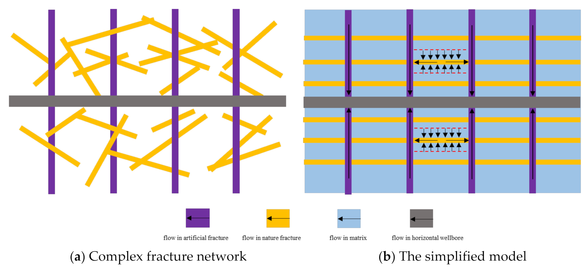
2.1. Physical Model and Assumption

After large-scale hydraulic fracturing in a tight reservoir, a complex fracture network is formed near horizontal wells [24,25]. Figure 1 demonstrates the physical model of the multistage fractured horizontal well: Figure 1a presents a multistage fractured horizontal well in an infinite reservoir. The natural fracture and the main fracture cross each other to form a fracture network. Figure 1b shows the simplified physical model, which assumes that the fluid flows from the matrix to the main fracture, and then from the main fracture to the wellbore. The fluid in the matrix does not flow directly to the wellbore.

In the simplified model, each main fracture possesses the same geometry, seepage parameters, and natural fractures. Other hypotheses include: (1) the pore medium of the reservoir deforms as the effective stress varies; (2) the fluid is micro compressible without any special physical and chemical phenomena; (3) the conductivity of fractures is limited and that of horizontal wells is unlimited; and (4) gravity and capillary pressure are neglected.

2.2. Mathematical Model with Stress Sensitivity Effect

The previous studies have unraveled that with formation pressure varying, the pore fracture media of different sizes shrink and deform, a stress sensitive effect existing [26,27]. In this paper, an exponential expression is applied to describe the stress sensitivity effect in tight reservoirs [28]:

$$k_{stress}=k_0{e}^{-\alpha \left(p_0-p\right)}$$

(1)

In this, $k_{stress}$ is permeability considering stress sensitivity, mD; $\alpha$ is the stress sensitivity coefficient, MPa⁻¹; $p$ is the reservoir pressure, MPa; and the subscript 0 denotes the initial state.

According to the conservation of mass, the fluid continuity equation can be expressed as

$$-\nabla \cdot \left({\rho }_l{\overrightarrow{v}}_l\right)=\frac{\partial }{\partial t}\left(\varphi {\rho }_l{S}_l\right)$$

(2)

In Equation (2), $\rho$ represents density, kg/m³, and the subscript $l$ represents the fluid phase (oil or water).

According to Darcy’s law and the reservoir stress sensitivity effect, the multiphase fluid seepage velocity can be expressed as

$${\overrightarrow{v}}_l=-\frac{k_{stress}{k}_{rl}}{{\mu }_l}\left(\nabla p_l-{\rho }_{l}g\right)$$

(3)

The reservoir temperature model for single-phase flow has been developed previously [29]. The former reservoir temperature model can be extended to tight oil reservoirs:

$$\begin{array}{l}{\displaystyle \sum _l\rho C_{pl}\frac{\partial T}{\partial t}-}{\displaystyle \sum _l\left(\varphi S_l{\beta }_l\frac{\partial p_l}{\partial t}\right)T}={\displaystyle \sum _l\left({\rho }_l\frac{k_{stress}{k}_{rl}}{{\mu }_l}\cdot C_{pl}\nabla p_l\right)}\nabla T\\ -{\displaystyle \sum _l\left\{\frac{k_{stress}{k}_{rl}}{{\mu }_l}\left({\beta }_{l}T-1\right)\cdot {\left(\nabla p_l\right)}^2\right\}}+K_T·{\nabla }^{2}T+q_{wb}\end{array}$$

(4)

In Equation (4), $C_{pl}$ represents the specific heat of reservoir fluid, J/(kg °C); $k_{rl}$ represents the relative permeability; $S_l$ represents saturation; ${\beta }_l$ represents the coefficient of thermal expansion, 1/°C; ${\mu }_l$ represents dynamic viscosity, mPa.s; and $K_T$ represents the heat transfer coefficient of the reservoir, W/(m·°C). Each term in Equation (4) is expressed as: energy change term in reservoir, energy change term due to fluid thermal expansion, thermal convection term, thermal expansion term and viscous dissipation term, and the heat conduction and heat transfer between reservoir and wellbore, where $q_{wb}$ is the heat transfer rate between the cementing section and the wellbore.

Similarly, the fracture temperature model can be derived:

$${\displaystyle \sum _l\rho C_p\frac{\partial T_f}{\partial t}-}{\displaystyle \sum _l\left({\varphi }_f{S}_{fl}{\beta }_{fl}\frac{\partial p_{fl}}{\partial t}\right)T_f}={\displaystyle \sum _l\frac{{\rho }_{fl}{k}_F{k}_{frl}{C}_{pl}}{{\mu }_l}}\left(\frac{\partial p_{fl}}{\partial y}\frac{\partial T_f}{\partial y}\right)-{\displaystyle \sum _l\left\{\frac{k_f{k}_{frl}}{{\mu }_l}\left({\beta }_{fl}{T}_f-1\right){\left(\frac{\partial p_{fl}}{\partial y}\right)}^2\right\}}+K_{Tf}\left(\frac{{\partial }^2{T}_f}{\partial y^2}\right)$$

(5)

In Equation (5), the geometric dimension of the fracture width is small, so the flow in the direction of the fracture width is neglected [29], and the subscript $f$ denotes fracture. $T_f$ denotes the fracture temperature,·°C; $p_f$ denotes the fracture pressure, MPa; and $K_{Tf}$ denotes the fracture heat transfer coefficient, J/(m·s·K).

Based on energy conservation, the wellbore temperature variation is expressed by the wellbore temperature model:

$$\frac{dT}{dx}=\frac{dp}{dx}\frac{{\displaystyle \sum _l{\rho }_l{v}_l{y}_l{C}_{pl}{K}_{JT,l}}}{{\displaystyle \sum _l{\rho }_l{v}_l{y}_l{C}_{pl}}}+\frac{2}{R}\left(T_I-T\right)\left[\frac{\gamma {\displaystyle \sum _l{\rho }_{l,I}{v}_{l,I}{y}_{l,I}{C}_{p,l}+\left(1-\gamma \right){\alpha }_T}}{{\displaystyle \sum _l{\rho }_l{v}_l{y}_l{C}_{pl}}}\right]-\frac{{\displaystyle \sum _l{\rho }_l{v}_l{y}_l}}{{\displaystyle \sum _l{\rho }_l{v}_l{y}_l{C}_{pl}}}g\sin \theta$$

(6)

In Equation (6), the subscript I indicates inflow (reservoir fluid flowing into the wellbore); $T_I$ indicates reservoir inflow temperature, °C; R indicates pipe inner diameter, m; $y_l$ indicates liquid holdup; $K_{JT}$ indicates the Joule–Thomson coefficient, °C/MPa; and ${\alpha }_T$ indicates total heat transfer coefficient, W/(m²·°C). $\gamma$ indicates the degree of the wellbore opening; $\gamma =1$ at the fracture, and $\gamma =0$ at the cementing section [30]. When the reservoir and the wellbore model are coupled, the diameter of the wellbore is much smaller than the size of the divided grid, and the grid containing the wellbore cannot directly describe the flow and heat exchange between the wellbore and the reservoir grid block. Hence, an equivalent radius is introduced to describe the flow between the reservoir grid block and the wellbore [31]:

$$r_{eff}=0.28\frac{\left[{\left(\frac{k_y}{k_x}\right)}^{\frac{1}{2}}\mathrm{\Delta }{x}^2+{\left(\frac{k_x}{k_y}\right)}^{\frac{1}{2}}\mathrm{\Delta }{y}^2\right]}{{\left(\frac{k_y}{k_x}\right)}^{\frac{1}{4}}+{\left(\frac{k_x}{k_y}\right)}^{\frac{1}{4}}}$$

(7)

The heat exchange between the reservoir and wellbore can be expressed as

$$K_T{\left.\frac{dT}{dr}\right|}_{r=r_w}=U_T\left({\left.T_{res}\right|}_{r=r_w}-T_w\right)$$

(8)

In Equation (8), $T_{res}$ and $T_w$ are reservoir and wellbore temperature, and $U_T$ is the overall heat transfer coefficient between the wellbore and the formation. Putting the wellbore surface area (${\left.A\right|}_{r=r_{eff}}$, m²) and the overall heat transfer coefficient (${\left.U_T\right|}_{r=r_{eff}}$) of the effective radius into the above equation indicates the heat transfer from the reservoir to the wellbore. The following results can be obtained:

$$q_{wb}={\left.A\right|}_{r=r_{eff}}{\left.U_T\right|}_{r=r_{eff}}\left(T_w-{\left.T_{res}\right|}_{r=r_{eff}}\right)$$

(9)

2.3. Boundary Conditions and Initial Conditions

The reservoir can be regarded as a closed rectangle. The equation of the boundary condition is

$${\left.\frac{\partial p\left(x,y\right)}{\partial x}\right|}_{x=x_L}={\left.\frac{\partial p\left(x,y\right)}{\partial y}\right|}_{y=y_L}=0$$

(10)

$${\left.\frac{\partial T\left(x,y\right)}{\partial x}\right|}_{x=x_L}={\left.\frac{\partial T\left(x,y\right)}{\partial y}\right|}_{y=y_L}=0$$

(11)

In this, X_L, Y_L represents the boundaries of X and Y directions.

At the start of production, the initial pressure distribution and temperature distribution in the reservoir were the initial conditions of the model:

$${\left.p\right|}_{t=0}=p_i$$

(12)

$${\left.T\right|}_{t=0}=T_i$$

(13)

In Equations (12) and (13), $p_i$ and $T_i$ represent the initial formation pressure and temperature before production. The above governing equations, boundary conditions, and initial conditions constitute the mathematical model of the research problem.

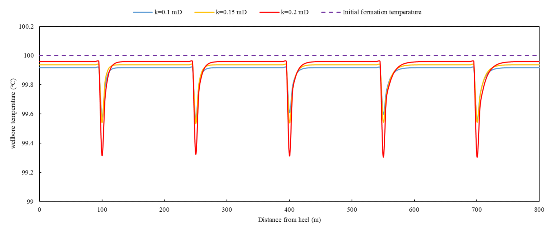
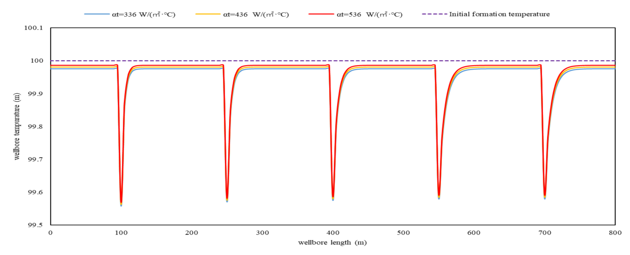
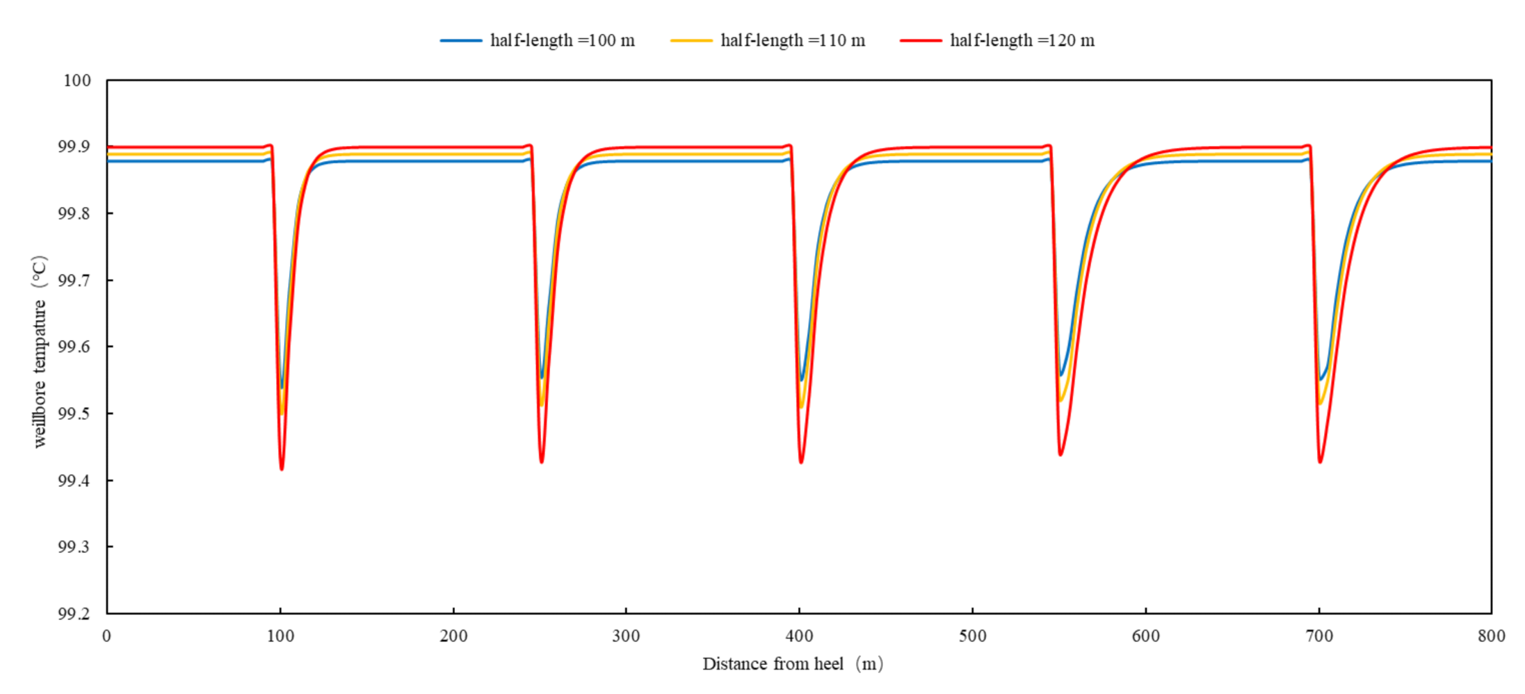
3. Analysis of Wellbore Temperature Sensitivity Factors

According to the mathematical model established in the previous section, the variation of the wellbore temperature profile is affected by multiple factors simultaneously [32]. Therefore, the sensitivity analysis of the multistage fractured horizontal well temperature profiles in tight reservoirs is performed to determine the main controlling factors affecting wellbore temperature. A multistage fractured horizontal well in the flowback stage was set to produce at a constant rate of oil-water production for 15 days. The initial conditions and other parameters are shown in

Table 1. The fracture and calculation parameters for analysis.

Parameter	Unit	Value
Formation porosity	/	0.1
Formation permeability	mD	0.2
Formation temperature	°C	100
Initial reservoir pressure	MPa	20
Rock heat capacity	J/(kg·°C)	1264
Rock heat conductivity	W/(m·°C)	1.3
Oil density	kg/m3	0.641 × 103
Oil viscosity	mPa.s	0.8
Oil specific heat	J/(kg·°C)	2193
Oil thermal conductivity	W/(m·°C)	3.46
Water density	kg/m3	1.0 × 103
Water viscosity	mPa.s	0.317
Water heat capacity	J/(kg·°C)	4194
Water heat conductivity	W/(m·°C)	4.32
Wellhead temperature	°C	14.7
Wellbore length	m	800
Pipe inner	m	0.01
Fracture permeability	D	0.9
Fracture half-length	m	100
Fracture width	m	0.002

.

Figure 2 indicates that the reservoir pressure decreases with the production process over a 15-day period. Apparently, the reservoir pressure distribution demonstrates the distinct trait of horizontal multistage fractured well production. Reservoir fluids flow into the well only through fractures, which induces a major pressure drop. Figure 3 reveals the variation of wellbore temperature for different stress sensitivity coefficients. $\mathrm{\Delta }T$ is the discrepancy between the fracture temperature and initial reservoir temperature. As shown in Figure 3: (1) In the flowback stage, the temperature of the water (fracturing fluid) is actually lower than that of the oil at the same layer due to the difference of the Joule–Thomson coefficient. Therefore, the oil-water two-phase flow into the wellbore will entail a decrease in the wellbore temperature. (2) When the stress sensitivity is taken into account, the permeability at the fracture diminishes and the production pressure difference enlarges, which amplifies the Joule–Thomson effect on oil temperature, so the temperature variation decreases when flowing into the wellbore.

Figure 4 demonstrates the variation of the wellbore temperature profile with different water cuts. As the water production increases, the wellbore temperature profile decreases gradually. During the flowback stage, the water-producing zone is marked by the temperature drop at the fractures [33]. The temperature drop at the fracture becomes more pronounced as the water production increases.

Assuming the formation permeability of 0.1 mD, 0.15 mD, and 0.2 mD, and other parameters remaining constant, the coupled thermal model is applied to simulate the temperature distribution of the well. Figure 5 indicates that the higher the formation permeability, the smaller the production pressure difference. Thus, the oil temperature change caused by the Joule–Thomson effect is smaller, the cooling effect of water in the two-phase flow is more conspicuous, and the temperature at the fractures declines more [34].

Figure 6 demonstrates that the wellbore temperature profile increases with the increase in the total thermal conductivity of the reservoir. However, since the total thermal conductivity does not influence the pressure distribution in the reservoir, the total thermal conductivity of different reservoirs has little impact on the temperature decline of the wellbore temperature profile at the fractures [35].

The fracture parameters affecting the wellbore temperature profile of fractured horizontal wells are fracture half-length and fracture conductivity [36]. Assuming other parameters are constant, the temperature distribution of the fractured horizontal well with fracture half-length of 100 m, 110 m, and 120 m is simulated using the above coupled temperature model. As shown in Figure 7, a positive correlation exists between inflow temperature and fracture half-length. With the increase of the fracture half-length, the cooling effect of water becomes more significant, which contributes to a decrease in wellbore temperature.

Hypothesizing that the conductivity of fractures formed after fracturing is 10 md cm, 15 md cm, and 20 md cm, and other parameters remaining constant, the temperature distribution profiles of the fractured horizontal well with different conductivity coefficients are simulated in Figure 8. As the fracture conductivity coefficient increases, the flow resistance of fluid in the fracture decreases, and the heat loss due to viscous dissipation decreases. Hence, the inflow temperature at the fracture location rises appreciably.

The orthogonal experimental analysis method is introduced to determine the main controlling factors of horizontal wellbore temperature profile [37]. The orthogonal analysis table is established by selecting five factors, comprising: the water production rate $Q_w$, formation permeability $k$, total thermal conductivity ${\alpha }_t$, fracture half-length $L_f$, and fracture conductivity $FCD$. Each factor consists of three different experimental parameters, as shown in

Table 2. Analysis factors of orthogonal experiment.

No.	${\mathit{Q}}_{\mathit{w}}$ m³/d	$\mathit{k}$ mD	${\mathit{\alpha }}_{\mathit{t}}$ W/(m2·K)	${\mathit{L}}_{\mathit{f}}$ m	$\mathit{F}\mathit{C}\mathit{D}$ mD·m
1	0	0.1	336	40	10
2	5	0.15	436	60	15
3	10	0.2	536	70	20

. During the orthogonal test analysis, the half-length of each fracture is assumed to be equal, and the average value of the discrepancy between the initial formation temperature and the wellbore temperature at each fracture position is adopted as the test index. The average value of the temperature difference basically reflects the degree of overall temperature reduction with different factors as the formation fluid flows from the reservoir boundary into the wellbore.

Sixteen groups of experiments were completed based on the data in Table 2 and the principles of orthogonal experiment design. The orthogonal design and results are shown in

Table 3. The orthogonal experimental design and results.

No.	${\mathit{Q}}_{\mathit{w}}$	$\mathit{k}$	${\mathit{\alpha }}_{\mathit{t}}$	${\mathit{L}}_{\mathit{f}}$	$\mathit{F}\mathit{C}\mathit{D}$	$\mathrm{\Delta }\mathit{T}$
1	2	1	3	3	1	0.276
2	1	1	1	1	1	0.314
3	1	3	1	2	1	0.344
4	2	1	1	1	3	0.282
5	1	2	3	1	3	0.256
6	3	2	2	1	1	0.373
7	2	2	1	2	2	0.356
8	3	1	1	1	2	0.295
9	1	1	2	2	3	0.309
10	3	3	1	3	3	0.336
11	1	2	1	3	1	0.324
12	2	3	2	1	1	0.261
13	1	1	2	3	2	0.336
14	1	1	1	1	1	0.288
15	3	1	3	2	1	0.326
16	1	3	3	1	2	0.355
K1	0.316	0.303	0.317	0.303	0.313	/
K2	0.294	0.327	0.320	0.334	0.336	/
K3	0.333	0.324	0.303	0.318	0.296	/
R	0.039	0.024	0.017	0.031	0.022	/
Result	$L_f$ > $Q_w$ > $k$ > $FCD$ > ${\alpha }_t$

. The results of the range analysis indicate that the influence of each single factor on the temperature profile of fractured horizontal wells, in descending order, is as follows: $L_f$ > $Q_w$ > $k$ > $FCD$ > ${\alpha }_t$. The principal factors affecting the temperature profile of fractured horizontal wells are fracture half-length, water production, and reservoir permeability.

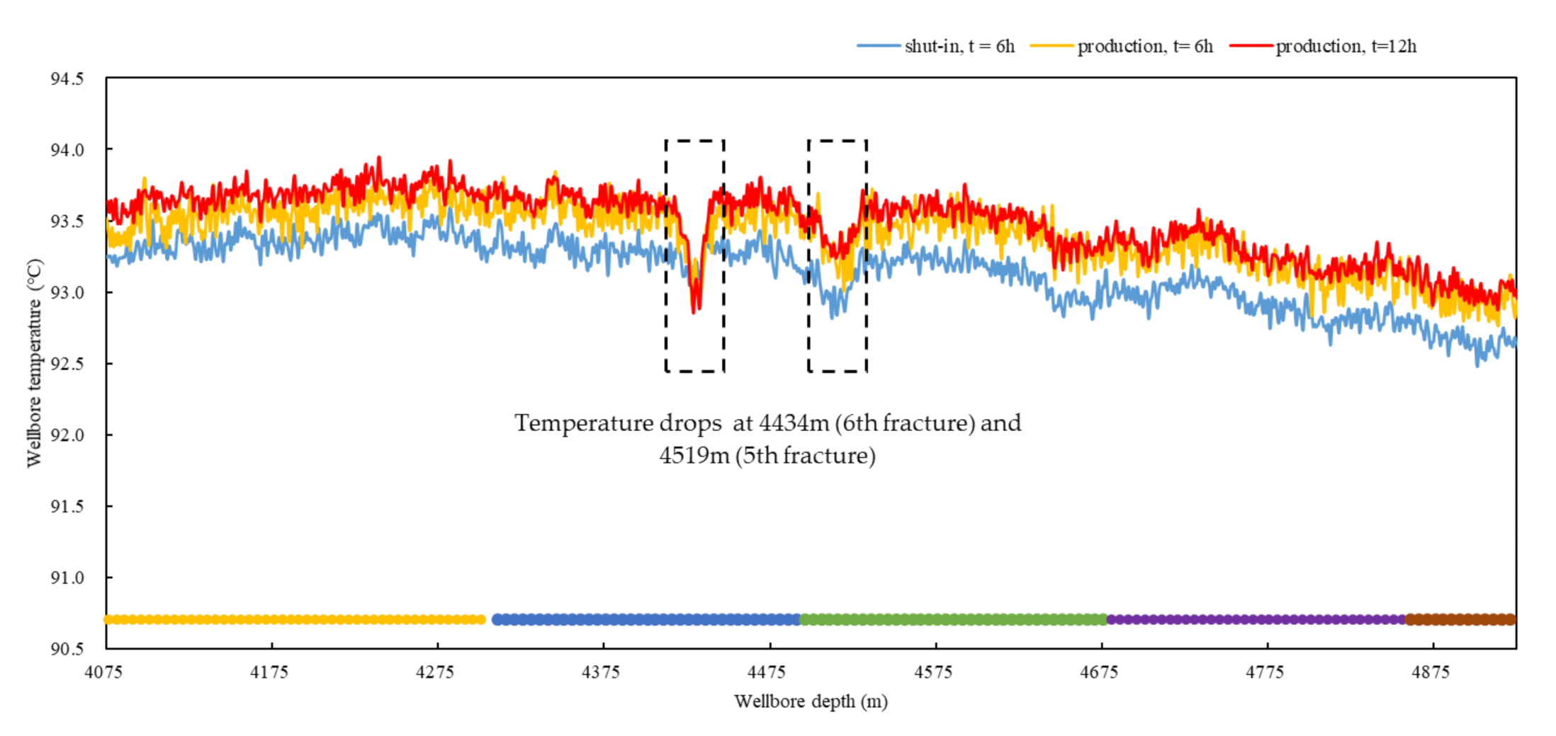
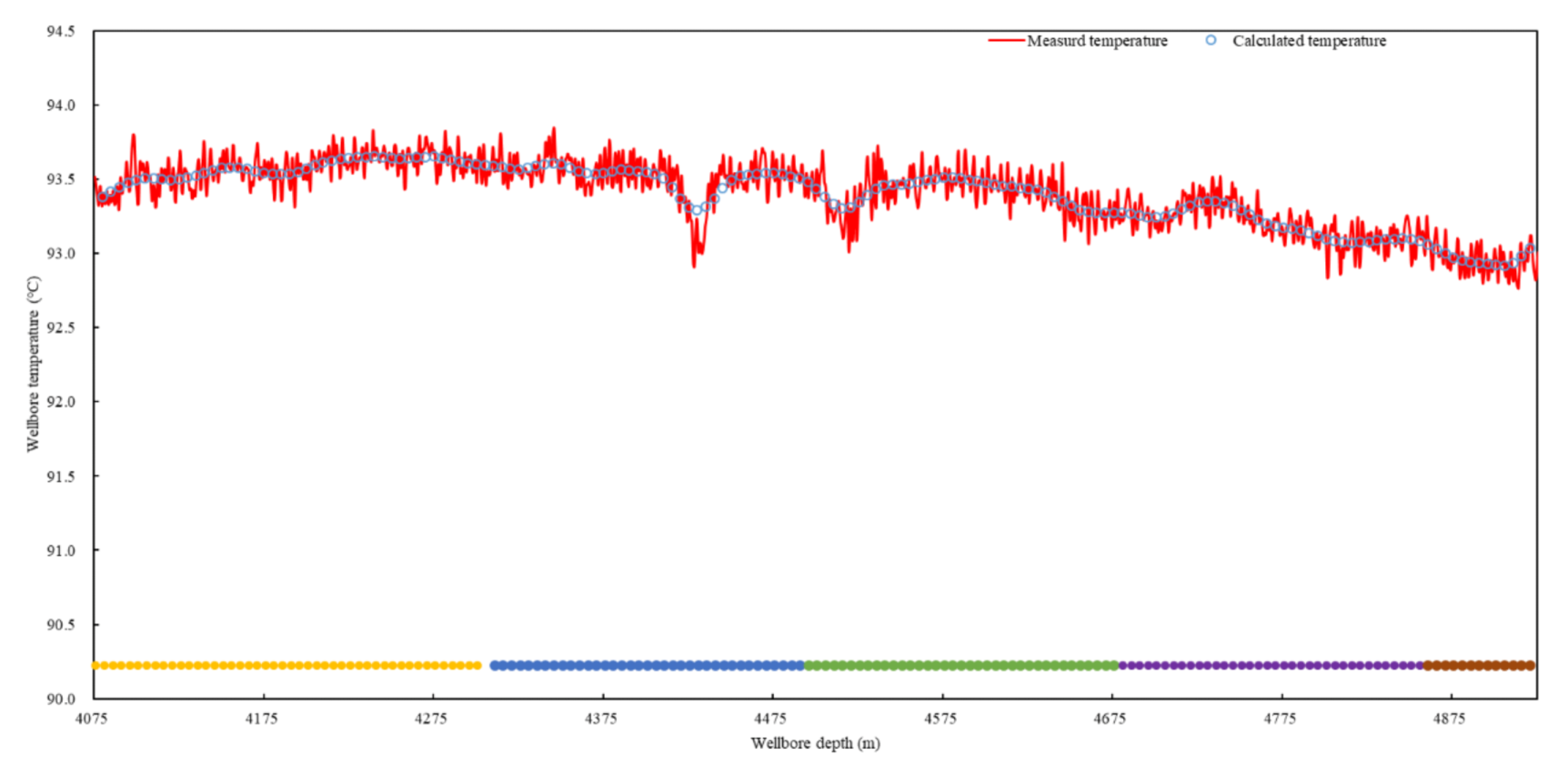
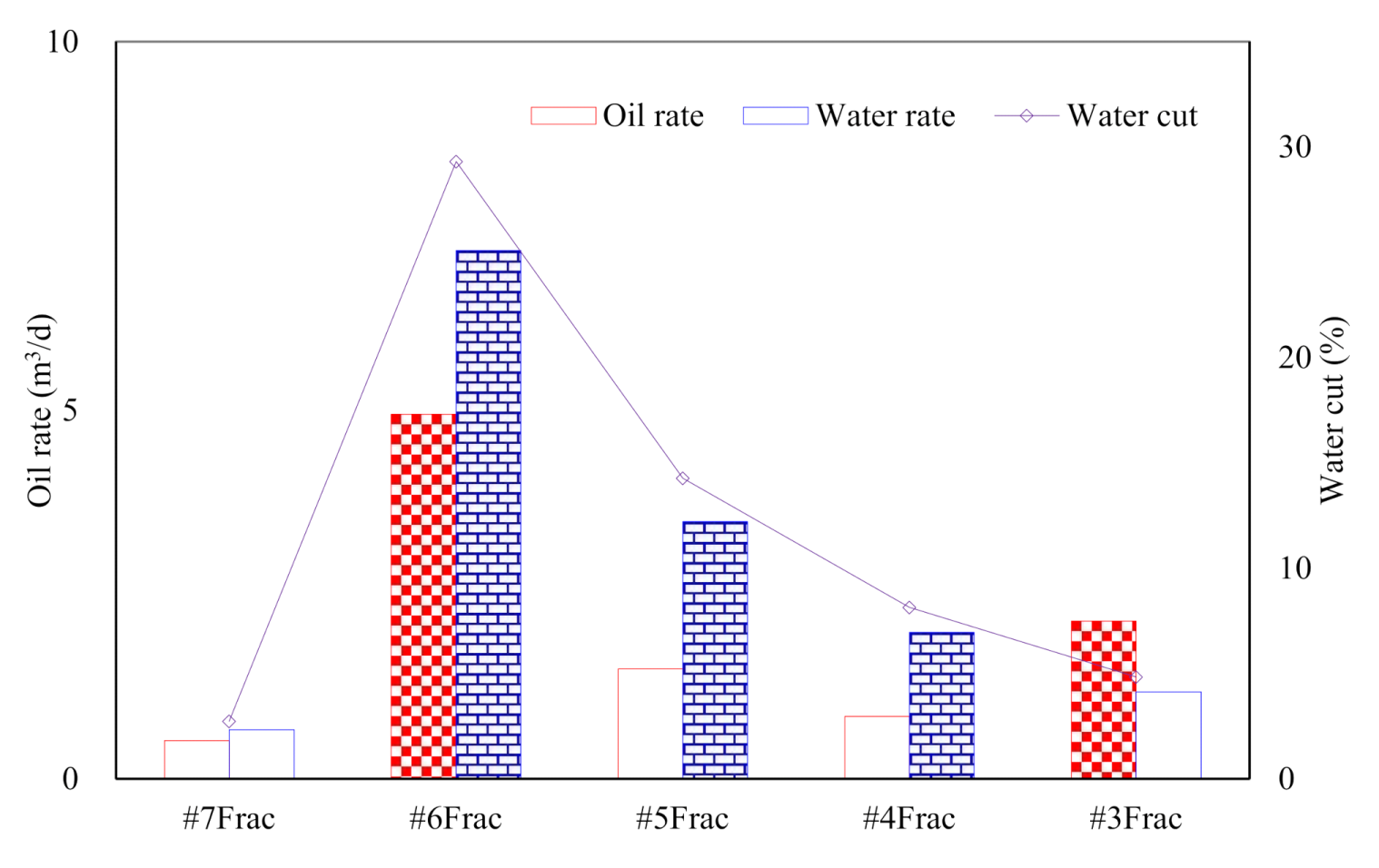
4. Field Application

The temperature prediction model for a multistage fractured horizontal well with stress sensitivity established in Section 2 predicts the temperature profile of a tight oil fractured horizontal well. M1 is a tight oil reservoir multistage fractured horizontal well in the Junggar Basin. The relevant parameters of this well are shown in

Table 4. The relevant parameters of M1 well.

Wellbore Length (m).	1174
Porosity (%)	0.1
Formation permeability (mD)	0.037
Initial reservoir pressure (MPa)	51.67
Initial reservoir temperature (°C)	92.43
Fracture length (m)	120
Fracture permeability (D)	0.9

. The temperature profile of M1 well 4075 m (7th fracture)–4930.3 m (3rd fracture) in the shut-in and production stage was measured by DTS, as shown in Figure 9.

In Figure 9, the wellbore temperature in the shut-in phase was stable at 92.9~93.8 °C. Affected by the fracturing fluid entering the ground, the temperature dropped significantly at 4434 m (sixth fracturing stage) and 4519 m (fifth fracturing stage). After the well is opened and produced with a 3.5 mm nozzle, the temperature of the horizontal section is declined by the cold fluid (fracturing fluid) produced. Compared to the shut-in stage, the temperature of the wellbore drops by 0.2–1.1 °C. The temperature distribution of the wellbore at 4434 m (6th fracture) and 4519 m (5th fracture) showed a significant negative anomaly.

The shut-in temperature is applied as the initial formation temperature, and the borehole trajectory, geothermal gradient, formation, and fluid parameters are input. The constructed temperature model is fitted to the DTS data at t = 6 h, with the flow rate of 25 m³/d. The measured data and fitted data are shown in Figure 10, which indicates that the simulated calculation result fits well with the measured temperature, and the temperature change trend from the toe to the root of the wellbore is consistent. The inflow of low-temperature fluid leads to the decline of 4434 m (6th fracture) and 4519 m (5th fracture), and the thermal convection effect plays a dominant role. According to the temperature fitting results, the production profile of each fracture in Well M1 can be inverted. As shown in Figure 11, the 3rd, 5th, and 6th stage fractures are the main production zones in the horizontal well.

5. Conclusions

In this paper, a novel temperature prediction model for a multistage fractured horizontal well is established with consideration of the stress sensitivity of a tight reservoir. In the present model, two-phase flow and the Joule–Thomson are also considered. According to the model calculation results and orthogonal test analysis: (1) After hydraulic fracturing, a large amount of cryogenic fluid enters the reservoir. During the production of the horizontal well, water (fracturing fluid) flows into the wellbore, resulting in a decrease in wellbore temperature. (2) The fracture half-length, water production, and formation permeability have been identified as the main factors affecting the wellbore temperature of two-phase flow multistage fractured horizontal wells in a tight reservoir. (3) The model was applied to interpret the DTS temperature profile of a multistage fractured horizontal well in a tight oil reservoir. The calculated temperature of the model matches well with the measured temperature and determines the production of each fracture.

References

1. Tang, Y.; Liang, B. Reservoir Surveillance Pilot Study for Midland Basin Tight Oil Spacing Optimization. In Proceedings of the SPE Liquids-Rich Basins Conference—North America, Midland, TX, USA, 2–3 September 2015. [Google Scholar] [CrossRef]
2. App, J. Permeability, skin, and inflow-profile estimation from production-logging-tool temperature traces. SPE J. 2017, 22, 1123–1133. [Google Scholar] [CrossRef]
3. Bilinchuk, A.V.; Ipatov, A.I.; Kremenetskiy, M.I. Evolution of production logging in low permeability reservoirs at horizontal wells, multiple-fractured horizontal wells and multilateral wells. Gazprom Neft experience (Russian). Neftyanoe khozyaystvo-Oil Industry 2018, 2018, 34–37. [Google Scholar] [CrossRef]
4. Zhu, D.; Hill, D.; Zhang, S. Using Temperature Measurements from Production Logging/Downhole Sensors to Diagnose Multistage Fractured Well Flow Profile//SPWLA 59th Annual Logging Symposium. OnePetro. 2018. Available online: https://onepetro.org/SPWLAALS/proceedings-abstract/SPWLA18/5-SPWLA18/D053S013R004/28837 (accessed on 10 June 2021).
5. Ouyang, L.B.; Belanger, D.L. Flow profiling by distributed temperature sensor (DTS) system-expectation and reality. SPE Prod. Oper. 2006, 21, 269–281. [Google Scholar] [CrossRef]
6. Holley, E.H.; Molenaar, M.M.; Fidan, E.; Banack, B. Interpreting uncemented multistage hydraulic-fracturing completion effectiveness by use of fiber-optic DTS injection data. SPE Drill. Completion 2013, 28, 243–253. [Google Scholar] [CrossRef]
7. Miller, D.E.; Coleman, T.; Zeng, X.; Patterson, J.R.; Reinschi, E.C.; Cardiff, M.A.; Wang, H.F.; Fratta, D.; Trainor-Guitton, W.; Thurber, C.H.; et al. DAS and DTS at Brady Hot Springs: Observations about coupling and coupled interpretations. In Proceedings of the 43rd Workshop on Geothermal Reservoir Engineering, Stanford, CA, USA, 12–14 February 2018. [Google Scholar]
8. Ramey, H.J., Jr. Wellbore heat transmission. J. Pet. Technol. 1962, 14, 427–435. [Google Scholar] [CrossRef]
9. Izgec, B.; Kabir, S.; Hasan, A.R. Transient fluid and heat flow modeling in coupled wellbore/reservoir systems. In Proceedings of the SPE Annual Technical Conference and Exhibition, San Antonio, TX, USA, 24–26 September 2006; Society of Petroleum Engineers: Houston, TX, USA, 2006. [Google Scholar]
10. Cheng, W.; Huang, Y.; Lu, D.; Yin, H. A novel analytical transient heat-conduction time function for heat transfer in steam injection wells considering the wellbore heat capacity. Energy 2011, 36, 4080–4088. [Google Scholar] [CrossRef]
11. Oldenburg, C.M.; Pan, L. Porous media compressed-air energy storage (PM-CAES): Theory and simulation of the coupled wellbore–reservoir system. Transp. Porous Media 2013, 97, 201–221. [Google Scholar] [CrossRef] [Green Version]
12. Onur, M.; Ulker, G.; Kocak, S.; Gok, I.M. Interpretation and analysis of transient-sandface-and wellbore-temperature data. SPE J. 2017, 22, 1156–1177. [Google Scholar] [CrossRef]
13. Sagar, R.; Doty, D.R.; Schmidt, Z. Predicting temperature profiles in a flowing well. SPE Prod. Eng. 1991, 6, 441–448. [Google Scholar] [CrossRef]
14. Hasan, A.R.; Kabir, C.S.; Lin, D. Analytic wellbore temperature model for transient gas-well testing. In Proceedings of the SPE Annual Technical Conference and Exhibition, Denver, CO, USA, 5–8 October 2003; Society of Petroleum Engineers: Houston, TX, USA, 2003. [Google Scholar]
15. Muradov, K.; Davies, D. Temperature transient analysis in horizontal wells: Application workflow, problems and advantages. J. Pet. Sci. Eng. 2012, 92, 11–23. [Google Scholar] [CrossRef]
16. Cui, J.; Yang, C.; Zhu, D.; Datta-Gupta, A. Fracture diagnosis in multiple-stage-stimulated horizontal well by temperature measurements with fast marching method. SPE J. 2016, 21, 2289–2300. [Google Scholar] [CrossRef]
17. Yoshida, N.; Zhu, D.; Hill, A.D. Temperature-prediction model for a horizontal well with multiple fractures in a shale reservoir. SPE Prod. Oper. 2014, 29, 261–273. [Google Scholar] [CrossRef]
18. Yoshida, N.; Hill, A.D.; Zhu, D. Comprehensive modeling of downhole temperature in a horizontal well with multiple fractures. SPE J. 2018, 23, 1580–1602. [Google Scholar] [CrossRef]
19. Sui, W.; Zhang, D.; Cheng, S.; Zou, Q.; Fu, X.; Ma, Z. Improved DTS profiling model for horizontal gas wells completed with the open-hole multi-stage fracturing system. J. Nat. Gas Sci. Eng. 2020, 84, 103642. [Google Scholar] [CrossRef]
20. Cao, Z.; Li, P.; Li, Q.; Lu, D. Integrated workflow of temperature transient analysis and pressure transient analysis for multistage fractured horizontal wells in tight oil reservoirs. Int. J. Heat Mass Transf. 2020, 158, 119695. [Google Scholar] [CrossRef]
21. Tian, X.; Cheng, L.; Cao, R.; Wang, Y.; Zhao, W.; Yan, Y.; Liu, H.; Mao, W.; Zhang, M.; Guo, Q. A new approach to calculate permeability stress sensitivity in tight sandstone oil reservoirs considering micro-pore-throat structure. J. Pet. Sci. Eng. 2015, 133, 576–588. [Google Scholar] [CrossRef]
22. Wu, Z.; Cui, C.; Lv, G.; Bing, S.; Cao, G. A multi-linear transient pressure model for multistage fractured horizontal well in tight oil reservoirs with considering threshold pressure gradient and stress sensitivity. J. Pet. Sci. Eng. 2019, 172, 839–854. [Google Scholar] [CrossRef]
23. Yu, Y.; Chen, Z.; Xu, J. A simulation-based method to determine the coefficient of hyperbolic decline curve for tight oil production. Adv. Geo-Energy Res. 2019, 3, 375–380. [Google Scholar] [CrossRef] [Green Version]
24. Yong, Y.K.; Maulianda, B.; Wee, S.C.; Mohshim, D.; Elraies, K.A.; Wong, R.C.K.; Gates, I.D.; Eaton, D. Determination of stimulated reservoir volume and anisotropic permeability using analytical modelling of microseismic and hydraulic fracturing parameters. J. Nat. Gas Sci. Eng. 2018, 58, 234–240. [Google Scholar] [CrossRef]
25. Cheng, L.; Wang, D.; Cao, R.; Xia, R. The influence of hydraulic fractures on oil recovery by water flooding processes in tight oil reservoirs: An experimental and numerical approach. J. Pet. Sci. Eng. 2020, 185, 106572. [Google Scholar] [CrossRef]
26. Nai, C.A.O.; Gang, L.E.I. Stress sensitivity of tight reservoirs during pressure loading and unloading process. Pet. Explor. Dev. 2019, 46, 138–144. [Google Scholar]
27. Wang, F.; Gong, R.; Huang, Z.; Meng, Q.; Zhang, Q.; Zhan, S. Single-phase inflow performance relationship in stress-sensitive reservoirs. Adv. Geo-Energy Res. 2021, 5, 202–211. [Google Scholar] [CrossRef]
28. Anyim, K.; Gan, Q. Fault zone exploitation in geothermal reservoirs: Production optimization, permeability evolution and induced seismicity. Adv. Geo-Energy Res. 2020, 4, 1–12. [Google Scholar] [CrossRef] [Green Version]
29. Ramazanov, A.S.; Nagimov, V.M. Analytical model for the calculation of temperature distribution in the oil reservoir during unsteady fluid inflow. Oil Gas Bus. J. 2007, 1, 1–8. [Google Scholar]
30. Yoshida, N. Modeling and Interpretation of Downhole Temperature in a Horizontal Well with Multiple Fractures. Ph.D. Thesis, Texas A&M University, College Station, TX, USA, 2016. [Google Scholar]
31. Peaceman, D.W. Interpretation of well-block pressures in numerical reservoir simulation with nonsquare grid blocks and anisotropic permeability. Soc. Pet. Eng. J. 1983, 23, 531–543. [Google Scholar] [CrossRef]
32. Yoshioka, K.; Zhu, D.; Hill, A.D.; Dawkrajai, P.; Wayne, L.L. Detection of water or gas entries in horizontal wells from temperature profiles//SPE Europec/EAGE Annual Conference and Exhibition. In Proceedings of the SPE Europec/EAGE Annual Conference and Exhibition, Vienna, Austria, 12–15 June 2006. [Google Scholar]
33. Li, Z.; Zhu, D. Predicting Flow Profile of Horizontal Well by Downhole Pressure and Distributed-Temperature Data for Waterdrive Reservoir. SPE Prod. Oper. 2010, 25, 296–304. [Google Scholar] [CrossRef]
34. App, J.F.; Yoshioka, K. Impact of reservoir permeability on flowing sandface temperatures: Dimensionless analysis. SPE J. 2013, 18, 685–694. [Google Scholar] [CrossRef]
35. Yoshioka, K.; Zhu, D.; Hill, A.D.; Dawkrajai, P.; Wayne, L.L. A comprehensive model of temperature behavior in a horizontal well. In Proceedings of the SPE Annual Technical Conference and Exhibition, Dallas, TX, USA, 9–12 October 2005. [Google Scholar]
36. Cui, J.; Zhu, D.; Jin, M. Diagnosis of multi-stage fracture stimulation in horizontal wells by downhole temperature measurements. In Proceedings of the SPE Annual Technical Conference and Exhibition, Amsterdam, The Netherlands, 27–29 October 2014. [Google Scholar]
37. Davim, J.P.; Reis, P.; Maranhao, C.; Jackson, M.J.; Cabral, J.; Gracio, J. Finite element simulation and experimental analysis of orthogonal cutting of an aluminium alloy using polycrystalline diamond tools. Int. J. Mater. Prod. Technol. 2010, 37, 46–59. [Google Scholar] [CrossRef]
Figure 1. Physical model of multistage fractured horizontal well in tight reservoir:(a) presents a multistage fractured horizontal well in an infinite reservoir; (b) shows the simplified physical model.
Energies 14 04760 g001
Figure 2. Reservoir pressure distribution of the multistage fractured horizontal well.
Energies 14 04760 g002
Figure 3. Wellbore temperature profiles and Δ T with different stress sensitivity coefficients.
Energies 14 04760 g003
Figure 4. Wellbore temperature profiles with different water cuts.
Energies 14 04760 g004
Figure 5. Wellbore temperature profiles with different permeability.
Energies 14 04760 g005
Figure 6. Wellbore temperature profiles with different thermal conductivity coefficients.
Energies 14 04760 g006
Figure 7. Wellbore temperature profiles with different fracture half-length.
Energies 14 04760 g007
Figure 8. Wellbore temperature profiles with different conductivity coefficients of fractures.
Energies 14 04760 g008
Figure 9. DTS measured data of horizontal well.
Energies 14 04760 g009
Figure 10. Measured and coupled model fitting data.
Energies 14 04760 g010
Figure 11. Production profile and water cut of each fracture.
Energies 14 04760 g011