
Solar-Based DG Allocation Using Harris Hawks Optimization While Considering Practical Aspects

 , , and
Abstract
:1. Introduction
Motivation and Contributions
- The proposed HHO has been tested with complex benchmark functions;
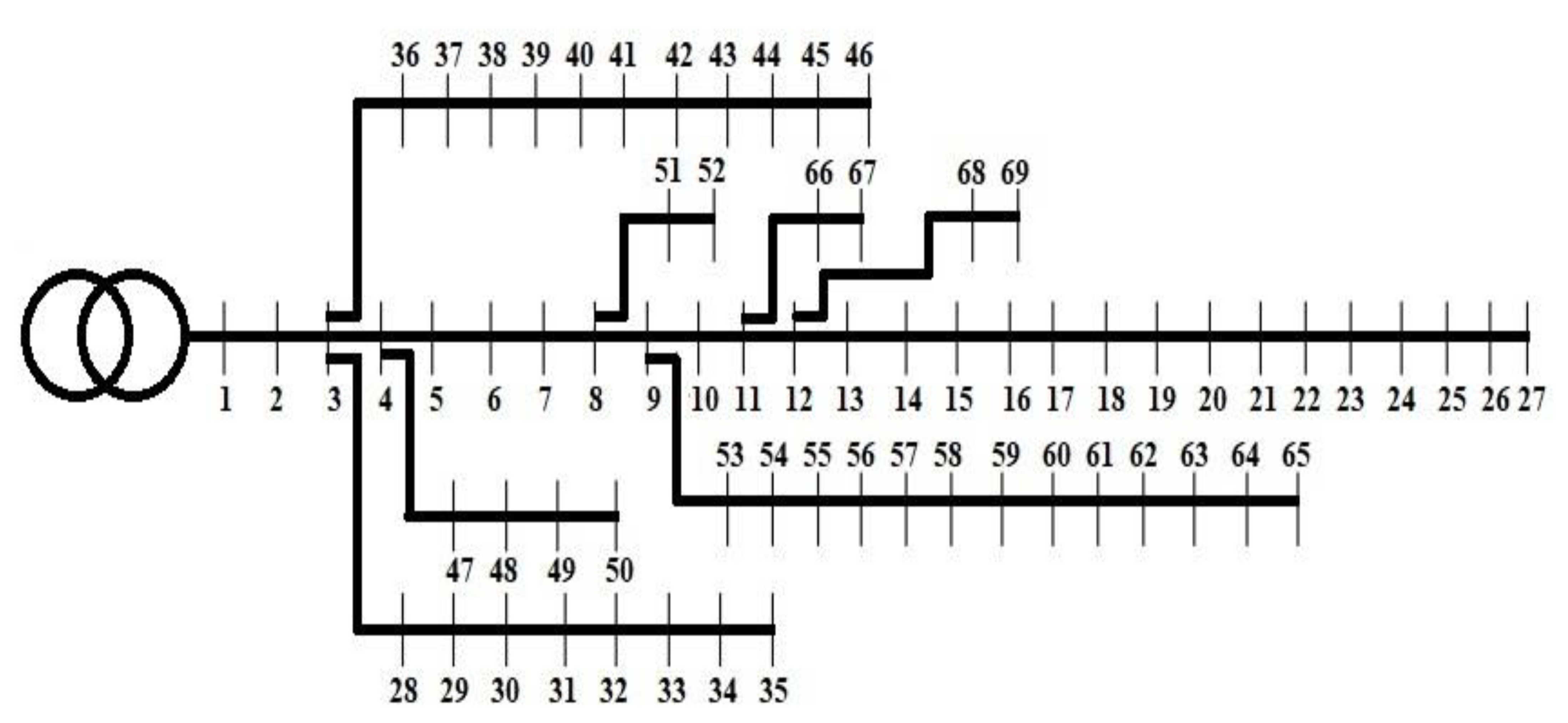
- Assign a novel approach for appropriate allocation and sizing of PV DGs in IEEE 33 bus and IEEE 69 bus power system network using HHO to minimize the power losses and improve the voltage profile;
- Compare the simulation outcomes of the proposed technique together with the recently available methods such as the teaching–learning-based optimization (TLBO), genetic algorithm (GA), particle swarm optimization (PSO), quasi-oppositional TLBO (QOTLBO), comprehensive teaching learning-based optimization (CTLBO), CTLBO ε-method, improved multiobjective elephant herding optimization (IMOEHO), improved decomposition-based evolutionary algorithm (I-DBEA), bat algorithm (BA), simulated annealing (SA), invasive weed optimization (IWO), bacterial foraging optimization algorithm (BFOA), and moth–flame optimization (MFO) to determine the effectiveness of the proposed algorithm over the exciting ones;
- Calculate the actual/practical size of the solar PV DG units to be installed to inject the targeted power into the power system grid.
2. Formulation of the Mathematical Problem
2.1. Loss Minimization
2.2. Practical Sizing of PV DG
3. Proposed HHO and Solution Approach
3.1. HHO: Features
3.2. Exploration Phase
3.3. Exploitation Phase
3.3.1. Soft Besiege
3.3.2. Hard Besiege
3.3.3. Soft Besiege along with Rapid Drives
3.3.4. Hard Besiege along with Rapid Drives
3.4. Solution Approch
3.4.1. HHO for PV DG Placement and Location
3.4.2. Computational Practice of HHO for DG Location and Values
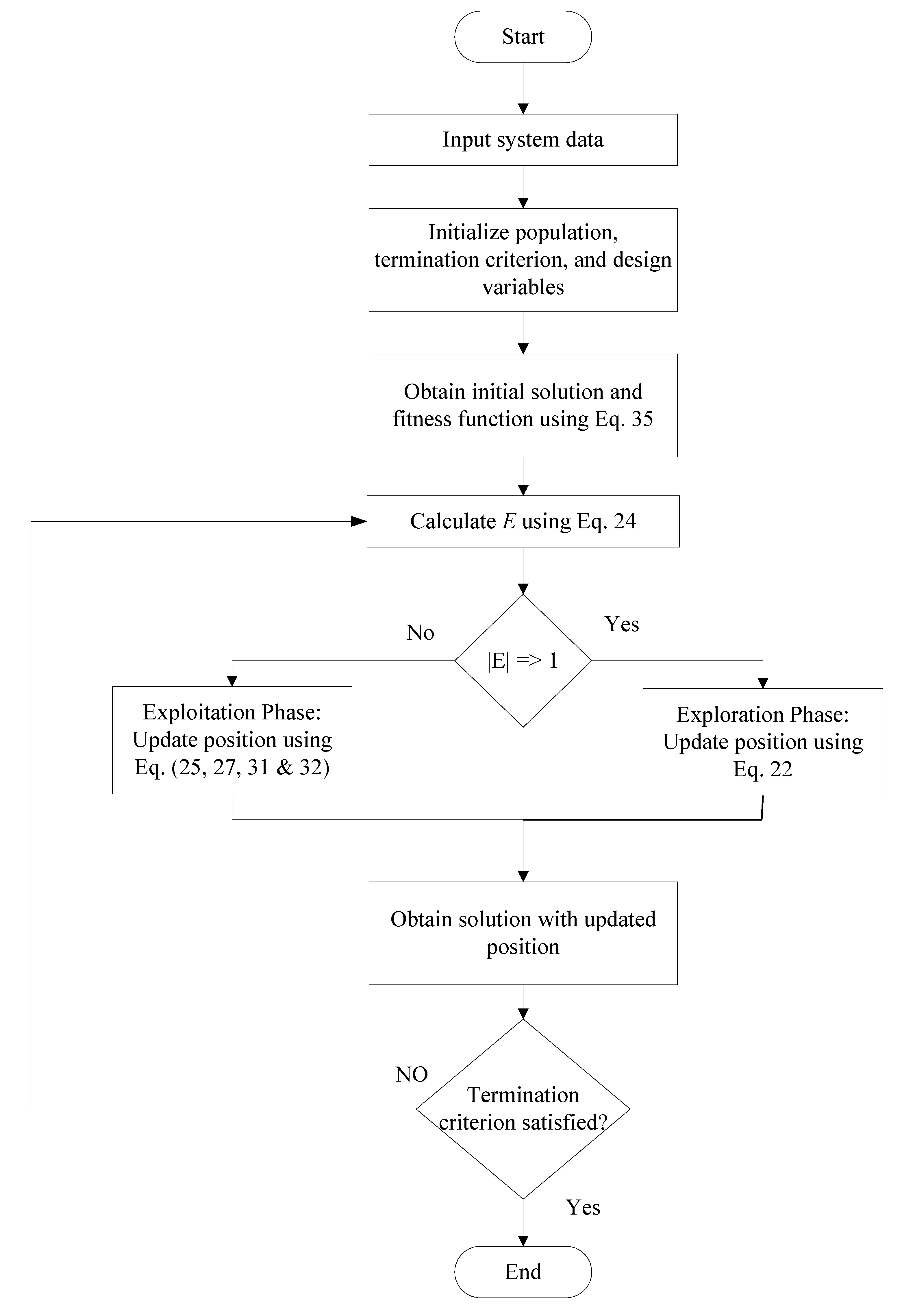
- Step 1
- Read the input data of the system, such as the maximum number of iterations, number of PV DG units, and population size.
- Step 2
- Generate the value of the size of PV DG within their upper (DGmax) and lower limits (DGmin). The same is shown in Equation (36).Here, DGi represents the size of ith DG unit. Now, constitute a vector Xj, that contains the possible locations (LOC) and size of DGs as mentioned in Equation (37).The LOC is generated randomly. Initial solution set X is then formulated as shown in Equation (38).
- Step 3
- Evaluation of the fitness function is processed using Equation (35) for individual Harris hawks, and the best hawk location is acknowledged.
- Step 4
- Calculate E using Equation (24).
- Step 5
- Exploration phase: Update the location of Harris hawks using Equation .
- Step 6
- Exploitation phase: Update the position using Equation
- Step 7
- Once the number of iterations reaches the maximum value, then terminate. Else, go back to Step 3.
4. Simulation Results and Discussions
4.1. Testing Strategies
4.2. Case 1
4.3. Case 2
4.4. Case 3
5. Practical PV DG Size Analysis
6. Conclusions
Author Contributions
Funding
Institutional Review Board Statement
Informed Consent Statement
Data Availability Statement
Conflicts of Interest
References
- Sandhya, K.; Chatterjee, K. A review on the state of the art of proliferating abilities of distributed generation deployment for achieving resilient distribution system. J. Clean. Prod. 2021, 287, 125023. [Google Scholar] [CrossRef]
- Wang, H.; Wang, J.; Piao, Z.; Meng, X.; Sun, C.; Yuan, G.; Zhu, S. The optimal allocation and operation of an energy storage system with high penetration grid-connected photovoltaic systems. Sustainability 2020, 12, 6154. [Google Scholar] [CrossRef]
- Sahib, J.T.; Ghani, A.R.M.; Jano, Z.; Mohamed, H.I. Optimum allocation of distributed generation using PSO: IEEE test case studies evaluation. Int. J. Appl. Eng. Res. 2017, 12, 2900–2906. [Google Scholar]
- Saad, N.M.; Sujod, M.Z.; Hui Ming, L.; Abas, M.F.; Jadin, M.S.; Ishak, M.R.; Abdullah, N.R.H. Impacts of photovoltaic distributed generation location and size on distribution power system network. Int. J. Power Electron. Drive Syst. 2018, 9, 905. [Google Scholar] [CrossRef]
- Jabr, R.A. Linear decision rules for control of reactive power by distributed photovoltaic generators. IEEE Trans. Power Syst. 2018, 33, 2165–2174. [Google Scholar] [CrossRef]
- Al-Ammar, E.A.; Farzana, K.; Waqar, A.; Aamir, M.; Saifullah; Ul Haq, A.; Zahid, M.; Batool, M. ABC algorithm based optimal sizing and placement of DGs in distribution networks considering multiple objectives. Ain Shams Eng. J. 2021, 12, 697–708. [Google Scholar] [CrossRef]
- Kumawat, A.; Singh, P. Optimal placement of capacitor and DG for minimization of power loss using genetic algorithm and artificial bee colony algorithm. Int. Res. J. Eng. Technol. 2016, 3, 2482–2488. [Google Scholar]
- Zakaria, Y.Y.; Swief, R.A.; El-Amary, N.H.; Ibrahim, A.M. Optimal distributed generation allocation and sizing using genetic and ant colony algorithms. J. Phys. Conf. Ser. 2020, 1447, 012023. [Google Scholar] [CrossRef]
- Sambaiah, K.S.; Jayabarathi, T. Loss minimization techniques for optimal operation and planning of distribution systems: A review of different methodologies. Int. Trans. Electr. Energy Syst. 2020, 30, e12230. [Google Scholar] [CrossRef] [Green Version]
- Hassan, A.A.; Fahmy, F.H.; Nafeh, A.E.-S.A.; Abu-elmagd, M.A. Hybrid genetic multi objective/fuzzy algorithm for optimal sizing and allocation of renewable DG systems: Genetic/Fuzzy Optimization of Renewable DGS. Int. Trans. Electr. Energy Syst. 2016, 26, 2588–2617. [Google Scholar] [CrossRef]
- Patel, D.K.; Singh, D.; Singh, B. Genetic algorithm-based multi-objective optimization for distributed generations planning in distribution systems with constant impedance, constant current, constant power load models. Int. Trans. Electr. Energy Syst. 2020, 30, e12576. [Google Scholar] [CrossRef]
- Almabsout, E.A.; El-Sehiemy, R.A.; An, O.N.U.; Bayat, O. A hybrid local search-genetic algorithm for simultaneous placement of DG units and shunt capacitors in radial distribution systems. IEEE Access 2020, 8, 54465–54481. [Google Scholar] [CrossRef]
- Vatani, M.; Solati Alkaran, D.; Sanjari, M.J.; Gharehpetian, G.B. Multiple distributed generation units allocation in distribution network for loss reduction based on a combination of analytical and genetic algorithm methods. IET Gener. Transm. Distrib. 2016, 10, 66–72. [Google Scholar] [CrossRef]
- Madhusudhan, M.; Kumar, N.; Pradeepa, H. Optimal location and capacity of DG systems in distribution network using genetic algorithm. Int. J. Inf. Technol. 2021, 13, 155–162. [Google Scholar]
- Ayodele, T.R.; Ogunjuyigbe, A.S.O.; Akinola, O.O. Optimal location, sizing, and appropriate technology selection of distributed generators for minimizing power loss using genetic algorithm. J. Renew. Energy 2015, 2015, 83291. [Google Scholar] [CrossRef] [Green Version]
- Sattianadan, D.; Sudhakaran, M.; Dash, S.S.; Vijayakumar, K.; Ravindran, P. Optimal placement of DG in distribution system using genetic algorithm. In Swarm, Evolutionary, and Memetic Computing, 1st ed.; Panigrahi, B.K., Suganthan, P.N., Das, S., Dash, S.S., Eds.; Springer International Publishing: Cham, Switzerland, 2013; Volume 8298, pp. 639–647. [Google Scholar]
- Liu, L.; Xie, F.; Huang, Z.; Wang, M. Multi-objective coordinated optimal allocation of DG and EVCSs based on the V2G mode. Processes 2020, 9, 18. [Google Scholar] [CrossRef]
- Hassan, A.S.; Sun, Y.; Wang, Z. Multi-objective for optimal placement and sizing DG units in reducing loss of power and enhancing voltage profile using BPSO-SLFA. Energy Rep. 2020, 6, 1581–1589. [Google Scholar] [CrossRef]
- Fan, Z.; Yi, H.; Xu, J.; Liu, P.; Hou, H.; Cui, R.; Xie, C. Multi-objective planning of DGs considering ES and EV based on source-load spatiotemporal scenarios. IEEE Access 2020, 8, 216835–216843. [Google Scholar] [CrossRef]
- Liu, W.; Xu, H.; Niu, S.; Xie, J. Optimal distributed generator allocation method considering voltage control cost. Sustainability 2016, 8, 193. [Google Scholar] [CrossRef] [Green Version]
- Azam Muhammad, M.; Mokhlis, H.; Naidu, K.; Amin, A.; Fredy Franco, J.; Othman, M. Distribution network planning enhancement via network reconfiguration and DG integration using dataset approach and water cycle algorithm. J. Mod. Power Syst. Clean Energy 2020, 8, 86–93. [Google Scholar] [CrossRef]
- Phuangpornpitak, W.; Bhumkittipich, K. Principle optimal placement and sizing of single distributed generation for power loss reduction using particle swarm optimization. Res. J. Appl. Sci. Eng. Technol. 2014, 7, 1211–1216. [Google Scholar] [CrossRef] [Green Version]
- Tolba, M.A.; Tulsky, V.N.; Zaki Diab, A.A. Optimal allocation and sizing of multiple distributed generators in distribution networks using a novel hybrid particle swarm optimization algorithm. In Proceedings of the 2017 IEEE Conference of Russian Young Researchers in Electrical and Electronic Engineering (EIConRus), St. Petersburg/Moscow, Russia, 1–3 February 2017. [Google Scholar]
- Raj, V.; Kumar, B.K. An improved affine arithmetic-based optimal DG sizing and placement algorithm using PSO for radial distribution networks with uncertainty. In Proceedings of the 2020 21st National Power Systems Conference (NPSC), Gandhinagar, India, 17–19 December 2020. [Google Scholar]
- Katyara, S.; Shaikh, M.F.; Shaikh, S.; Khand, Z.H.; Staszewski, L.; Bhan, V.; Majeed, A.; Shah, M.A.; Zbigniew, L. Leveraging a Genetic Algorithm for the optimal placement of distributed generation and the need for energy management strategies using a fuzzy inference system. Electronics 2021, 10, 172. [Google Scholar] [CrossRef]
- Barik, S.; Das, D.; Bansal, R.C. Zero bus load flow method for the integration of renewable DGs by mixed-discrete particle swarm optimisation-based fuzzy max–min approach. IET Renew. Power Gener. 2020, 14, 4029–4042. [Google Scholar] [CrossRef]
- Bohre, A.K.; Agnihotri, G.; Dubey, M. Optimal sizing and sitting of DG with load models using soft computing techniques in practical distribution system. IET Gener. Transm. Distrib. 2016, 10, 2606–2621. [Google Scholar] [CrossRef]
- Yahaya, A.A.; AlMuhaini, M.; Heydt, G.T. Optimal design of hybrid DG systems for microgrid reliability enhancement. IET Gener. Transm. Distrib. 2020, 14, 816–823. [Google Scholar] [CrossRef]
- Cheng, R.; Jin, Y. A competitive swarm optimizer for large scale optimization. IEEE Trans. Cybern. 2015, 45, 191–204. [Google Scholar] [CrossRef] [PubMed]
- Ganguly, S. Multi-objective planning for reactive power compensation of radial distribution networks with unified power quality conditioner allocation using particle swarm optimization. IEEE Trans. Power Syst. 2014, 29, 1801–1810. [Google Scholar] [CrossRef]
- Tolabi, H.B.; Ali, M.H.; Rizwan, M. Simultaneous Reconfiguration, Optimal Placement of DSTATCOM, and Photovoltaic Array in a Distribution System Based on Fuzzy-ACO Approach. IEEE Trans. Sustain. Energy. 2015, 6, 210–218. [Google Scholar] [CrossRef]
- Oloulade, A.; Imano Moukengue, A.; Agbokpanzo, R.; Vianou, A.; Tamadaho, H.; Badarou, R. New multi objective approach for optimal network reconfiguration in electrical distribution systems using modified ant colony algorithm. Am. J. Electr. Power Energy Syst. 2019, 8, 120. [Google Scholar] [CrossRef] [Green Version]
- Das, C.K.; Bass, O.; Kothapalli, G.; Mahmoud, T.S.; Habibi, D. Optimal placement of distributed energy storage systems in distribution networks using artificial bee colony algorithm. Appl. Energy 2018, 232, 212–228. [Google Scholar] [CrossRef]
- Seker, A.A.; Hocaoglu, M.H. Artificial Bee Colony algorithm for optimal placement and sizing of distributed generation. In Proceedings of the 2013 8th International Conference on Electrical and Electronics Engineering (ELECO), Bursa, Turkey, 28–30 November 2013. [Google Scholar]
- Yuvaraj, T.; Ravi, K. Multi-objective simultaneous DG and DSTATCOM allocation in radial distribution networks using cuckoo searching algorithm. Alex. Eng. J. 2018, 57, 2729–2742. [Google Scholar] [CrossRef]
- Arya, L.D.; Koshti, A. Modified shuffled frog leaping optimization algorithm based distributed generation rescheduling for loss minimization. J. Inst. Eng. (India) Ser. B 2018, 99, 397–405. [Google Scholar] [CrossRef]
- Rajaram, R.; Sathish Kumar, K.; Rajasekar, N. Power system reconfiguration in a radial distribution network for reducing losses and to improve voltage profile using modified plant growth simulation algorithm with Distributed Generation (DG). Energy Rep. 2015, 1, 116–122. [Google Scholar] [CrossRef] [Green Version]
- Othman, M.M.; El-Khattam, W.; Hegazy, Y.G.; Abdelaziz, A.Y. Optimal placement and sizing of distributed generators in unbalanced distribution systems using supervised big bang-big crunch method. IEEE Trans. Power Syst. 2015, 30, 911–919. [Google Scholar] [CrossRef]
- Yuvaraj, T.; Ravi, K.; Devabalaji, K.R. DSTATCOM allocation in distribution networks considering load variations using bat algorithm. Ain Shams Eng. J. 2017, 8, 391–403. [Google Scholar] [CrossRef] [Green Version]
- Duong, M.; Pham, T.; Nguyen, T.; Doan, A.; Tran, H. Determination of optimal location and sizing of solar photovoltaic distribution generation units in radial distribution systems. Energies 2019, 12, 174. [Google Scholar] [CrossRef] [Green Version]
- Al-Bazoon, M. Harris Hawks Optimization for optimum design of truss structures with discrete variables. Int. J. Math. Eng. Manag. Sci. 2021, 6, 1157–1173. [Google Scholar]
- Moayedi, H.; Osouli, A.; Nguyen, H.; Rashid, A.S.A. A novel Harris hawks’ optimization and k-fold cross-validation predicting slope stability. Eng. Comput. 2021, 37, 369–379. [Google Scholar] [CrossRef]
- Paital, S.R.; Ray, P.K.; Mohanty, S.R. A robust dual interval type-2 fuzzy lead-lag based UPFC for stability enhancement using Harris Hawks Optimization. ISA Trans. 2021. [Google Scholar] [CrossRef]
- Parsa, P.; Naderpour, H. Shear strength estimation of reinforced concrete walls using support vector regression improved by Teaching–learning-based optimization, Particle Swarm optimization, and Harris Hawks Optimization algorithms. J. Build. Eng. 2021, 44, 102593. [Google Scholar] [CrossRef]
- Bandyopadhyay, R.; Basu, A.; Cuevas, E.; Sarkar, R. Harris Hawks optimisation with Simulated Annealing as a deep feature selection method for screening of COVID-19 CT-scans. Appl. Soft Comput. 2021, 111, 107698. [Google Scholar] [CrossRef]
- Abd Elaziz, M.; Yousri, D. Automatic selection of heavy-tailed distributions-based synergy Henry gas solubility and Harris hawk optimizer for feature selection: Case study drug design and discovery. Artif. Intell. Rev. 2021, 54, 4685–4730. [Google Scholar] [CrossRef]
- Malik, A.; Tikhamarine, Y.; Sammen, S.S.; Abba, S.I.; Shahid, S. Prediction of meteorological drought by using hybrid support vector regression optimized with HHO versus PSO algorithms. Environ. Sci. Pollut. Res. Int. 2021, 28, 39139–39158. [Google Scholar] [CrossRef]
- Sharma, R.; Prakash, S. HHO-LPWSN: Harris hawks optimization algorithm for sensor nodes localization problem in wireless sensor networks. ICST Trans. Scalable Inf. Syst. 2018, 168807. [Google Scholar] [CrossRef]
- Gerey, A.; Sarraf, A.; Ahmadi, H. Groundwater single- and multiobjective optimization using Harris Hawks and Multiobjective Billiards-inspired algorithm. Shock Vib. 2021, 2021, 4531212. [Google Scholar]
- Setiawan, I.N.; Kurniawan, R.; Yuniarto, B.; Caraka, R.E.; Pardamean, B. Parameter optimization of support vector regression using Harris hawks optimization. Procedia Comput. Sci. 2021, 179, 17–24. [Google Scholar] [CrossRef]
- Mansoor, M.; Mirza, A.F.; Ling, Q. Harris hawk optimization-based MPPT control for PV systems under partial shading conditions. J. Clean. Prod. 2020, 274, 122857. [Google Scholar] [CrossRef]
- Seyfollahi, A.; Ghaffari, A. Reliable data dissemination for the Internet of Things using Harris hawks optimization. Peer Peer Netw. Appl. 2020, 13, 1886–1902. [Google Scholar] [CrossRef]
- Rodríguez-Esparza, E.; Zanella-Calzada, L.A.; Oliva, D.; Heidari, A.A.; Zaldivar, D.; Pérez-Cisneros, M.; Foong, L.K. An efficient Harris hawks-inspired image segmentation method. Expert Syst. Appl. 2020, 155, 113428. [Google Scholar] [CrossRef]
- Tikhamarine, Y.; Souag-Gamane, D.; Ahmed, A.N.; Sammen, S.S.; Kisi, O.; Huang, Y.F.; El-Shafie, A. Rainfall-runoff modelling using improved machine learning methods: Harris hawks optimizer vs. particle swarm optimization. J. Hydrol. 2020, 589, 125133. [Google Scholar] [CrossRef]
- Jia, H.; Peng, X.; Kang, L.; Li, Y.; Jiang, Z.; Sun, K. Pulse coupled neural network based on Harris hawks optimization algorithm for image segmentation. Multimed. Tools Appl. 2020, 79, 28369–28392. [Google Scholar] [CrossRef]
- Sammen, S.S.; Ghorbani, M.A.; Malik, A.; Tikhamarine, Y.; AmirRahmani, M.; Al-Ansari, N.; Chau, K.-W. Enhanced artificial neural network with Harris hawks optimization for predicting scour depth downstream of ski-jump spillway. Appl. Sci. 2020, 10, 5160. [Google Scholar] [CrossRef]
- Islam, M.Z.; Wahab, N.I.A.; Veerasamy, V.; Hizam, H.; Mailah, N.F.; Guerrero, J.M.; Mohd Nasir, M.N. A Harris Hawks Optimization based single- and multi-objective Optimal Power Flow considering environmental emission. Sustainability 2020, 12, 5248. [Google Scholar] [CrossRef]
- Khalifeh, S.; Akbarifard, S.; Khalifeh, V.; Zallaghi, E. Optimization of water distribution of network systems using the Harris Hawks optimization algorithm (Case study: Homashahr city). MethodsX 2020, 7, 100948. [Google Scholar] [CrossRef]
- Yousri, D.; Babu, T.S.; Fathy, A. Recent methodology based Harris Hawks optimizer for designing load frequency control incorporated in multi-interconnected renewable energy plants. Sustain. Energy Grids Netw. 2020, 22, 100352. [Google Scholar] [CrossRef]
- Abbasi, A.; Firouzi, B.; Sendur, P. On the application of Harris hawks optimization (HHO) algorithm to the design of microchannel heat sinks. Eng. Comput. 2021, 37, 1409–1428. [Google Scholar] [CrossRef]
- Teng, J.-H.; Luan, S.-W.; Lee, D.-J.; Huang, Y.-Q. Optimal charging/discharging scheduling of battery storage systems for distribution systems interconnected with sizeable PV generation systems. IEEE Trans. Power Syst. 2013, 28, 1425–1433. [Google Scholar] [CrossRef]
- Chakraborty, S.; Kumar, R. Comparative analysis of NOCT values for mono and multi C-Si PV modules in Indian climatic condition. World J. Eng. 2015, 12, 19–22. [Google Scholar] [CrossRef]
- Chakraborty, S. Reliable energy prediction method for grid connected photovoltaic power plants situated in hot and dry climatic condition. SN Appl. Sci. 2020, 2, 317. [Google Scholar] [CrossRef] [Green Version]
- Hassan, A.S.; Othman, E.A.; Bendary, F.M.; Ebrahim, M.A. Distribution systems techno-economic performance optimization through renewable energy resources integration. Array 2021, 9, 100050. [Google Scholar] [CrossRef]
- Mechanical Characteristics Electrical Characteristics PERC 350 Wp SPV MODULE. Available online: https://www.waaree.com/documents/WSMP-350_4BB_40mm_datasheet.pdf (accessed on 7 July 2021).
- Heidari, A.A.; Mirjalili, S.; Faris, H.; Aljarah, I.; Mafarja, M.; Chen, H. Harris hawks optimization: Algorithm and applications. Future Gener. Comput. Syst. 2019, 97, 849–872. [Google Scholar] [CrossRef]
- Zimmerman, R.D.; Murillo-Sánchez, C.E.; Thomas, R.J. MATPOWER: Steady state operations, planning, and analysis tools for power systems research and education. IEEE Tran. Power Systems 2011, 26, 12–19. [Google Scholar] [CrossRef] [Green Version]
- Sultana, S.; Roy, P.K. Multiobjective quasi-oppositional teaching learning based optimization for optimal location of distributed genera- tor in radial distribution systems. Int. J. Electr. Power Energy Syst. 2014, 63, 534–545. [Google Scholar] [CrossRef]
- Moradi, M.H.; Abedini, M. A combination of genetic algorithm and particle swarm optimization for optimal DG location and sizing in distribution systems. Int. J. Electr. Power Energy Syst. 2012, 34, 66–74. [Google Scholar] [CrossRef]
- Quadri, I.A.; Bhowmick, S.; Joshi, D. A comprehensive technique for optimal allocation of distributed energy resources in radial distribution systems. Appl. Energy 2018, 211, 1245–1260. [Google Scholar] [CrossRef]
- Meena, N.K.; Parashar, S.; Swarnkar, A.; Gupta, N.; Niazi, K.R. Improved elephant herding optimization for multiobjective DER accommodation in distri- bution systems. IEEE Trans. Ind. Inform. 2018, 14, 1029–1039. [Google Scholar] [CrossRef]
- Ali, A.; Keerio, M.U.; Laghari, J.A. Optimal site and size of distributed generation allocation in radial distribution network using multiobjective optimization. J. Mod. Power Syst. Clean Energy 2021, 9, 404–415. [Google Scholar] [CrossRef]
- Zimmerman, R.D.; Murillo-Sánchez, C.E. Matpower [Software]. 2020. Available online: https://matpower.org (accessed on 9 July 2021). [CrossRef]
- Injeti, S.K.; Prema Kumar, N. A novel approach to identity optimal access point and capacity of multiple DGs in a small, medium, and large scale radial distribution systems. Electr. Power Energy Syst. 2013, 45, 142–151. [Google Scholar] [CrossRef]
- Rama Prabha, D.; Jayabarathi, T. Optimal placement and sizing of multiple distributed generating units in distribution networks by invasive weed optimization algorithm. Ain Shams Eng. J. 2016, 7, 683–694. [Google Scholar] [CrossRef] [Green Version]
- Mohamed Imran, A.; Kowsalya, M. Optimal size and siting of multiple distributed generators in distribution system using bacterial foraging optimization. Swarm Evol. Comput. 2014, 15, 58–65. [Google Scholar] [CrossRef]
- Saleh, A.A.; Mohamed, A.-A.A.; Hemeida, A.M.; Ibrahim, A.A. Comparison of different optimization techniques for optimal allocation of multiple distribution generation. In Proceedings of the 2018 International Conference on Innovative Trends in Computer Engineering (ITCE), Aswan, Egypt, 19–21 February 2018. [Google Scholar]


| Year | Area of Application | Research Objectives | Research Findings | Reference No. |
|---|---|---|---|---|
| 2021 | Design of truss structures | The use of HHO to solve planar and spatial trusses with discrete design variables was investigated in this paper. Five benchmark structural issues were used to assess HHO’s performance, and the resultant designs were compared to 10 state-of-the-art algorithms. | The statistical results demonstrate that HHO is quite consistent and reliable when related to truss structure optimization. | [41] |
| 2021 | Prediction of slope stability | The study’s major goal is to develop a new metaheuristic optimization approach HHO for improving the accuracy of the traditional multilayer perceptron technique in estimating the factor of safety in the presence of inflexible foundations. Four slope stability conditioning elements are taken into account in this method: slope angle, rigid foundation position, soil strength, and applied surcharge. | The findings revealed that employing the HHO improves the ANN’s prediction accuracy while analyzing slopes with unknown circumstances. | [42] |
| 2021 | Power flow controller | To reduce oscillations in single and multimachine power systems, a HHO tuned dual interval type-2 fuzzy lead–lag (Dual-IT2FLL)-based universal power flow controller (UPFC) is suggested. The suggested damping controller uses speed deviation, a distant input signal for stability enhancement, to coordinate between the modulation index (MI) and phase angle of series and shunt converters of UPFC at the same time. | Different performance indicators (PIs) such as mean, standard deviation, overshoots, and settling time are used to demonstrate that the proposed HHO-tuned dual-IT2FLL-based UPFC outperforms others under various operating circumstances. | [43] |
| 2021 | Shear strength estimation of reinforced concrete walls | The authors suggested three novel models for estimating peak shear strength using a mix of support vector regression and metaheuristic optimization techniques including teaching–learning-based optimization (TLBO), PSO, and HHO. The authors compiled a huge database with 228 RC shear wall experimental data and eight input parameters. | The suggested models may be used to estimate the shear strength of RC shear walls, potentially improving the accuracy of forecasting the structure’s behavior and lowering construction costs. | [44] |
| 2021 | Screening of COVID-19 CT-scans | For the identification of COVID-19 from CT scan images, they suggested a two-stage pipeline consisting of feature extraction followed by feature selection (FS). A state-of-the-art convolutional neural network (CNN) model based on the DenseNet architecture was used for feature extraction. The HHO method was used in conjunction with SA and Chaotic initialization to remove noninformative and redundant features. The SARS-COV-2 CT-Scan dataset, which contains 2482 CT-scans, was used to test the suggested method. | The technique has an accuracy of about 98.42% without the chaotic initialization and the SA, which improves to 98.85% when the two are included, and therefore outperforms several state-of-the-art methods including other metaheuristic-based feature selection (FS) algorithms. The suggested approach reduces the number of characteristics chosen by around 75%, which is significantly better than most existing algorithms. | [45] |
| 2021 | Drug design and discovery | The authors presented a modified Henry gas solubility optimization (HGSO) based on heavy-tailed distributions (HTDs) utilizing improved HHO. A dynamical exchange between five HTDs were employed in this work to increase the HHO, which alters the exploitation phase in HGSO. | According to the values of accuracy, fitness value, and the number of selected characteristics, the results show that dynamic modified HGSO based on improved HHO has a high quality. | [46] |
| 2021 | Prediction of meteorological drought | In this study, the SVR (support vector regression) model was combined with two distinct optimization methods, PSO and HHO, to forecast the effective drought index (EDI) one month in advance in various sites across Uttarakhand, India. | The SVR-HHO model beat the SVR-PSO model in forecasting EDI, according to the results. SVR-HHO performed better than SVR-PSO in recreating the median, interquartile range, dispersion, and pattern of the EDI calculated from observed rainfall, according to visual assessment of model. | [47] |
| 2021 | Wireless sensor networks | The authors applied the HHO method to sensor node localization and compared their findings to other well-known optimization techniques that had just become available. | The suggested work’s simulation results revealed that it outperforms existing computational intelligence methods in terms of average localization error, number of localized sensor nodes, and computational cost. | [48] |
| 2021 | Groundwater | The HHO method was used to minimize the sum of absolute deviation between observed and simulated water-table levels in order to optimize hydraulic conductivity and specific yield parameters of a modular three-dimensional finite-difference (MODFLOW) groundwater model. | According to the findings, the Pareto parameter sets gave appropriate results when the maximum and minimum aquifer drawdown were defined in the range of –40 to +40 cm/year. | [49] |
| 2020 | Parameter optimization of support vector regression | The goal of this research is to look at the SVR approach that is optimized using HHO, also known as HHO-SVR. To establish the performance of the HHO-SVR, five benchmark datasets were used to assess it. The HHO method is also compared to various metaheuristic algorithms and kernel types. | The findings revealed that the HHO-SVR has almost the same performance as other techniques, but is less time efficient. | [50] |
| 2020 | MPPT control | This study offers a new MPPT controller based on HHO that successfully tracks maximum power in all weather situations. | The suggested HHO outperforms the competition in terms of maximum power point tracking (MPPT) and convergence at the global maximum power point. The HHO-based MPPT approach provides faster maximum power point (MPP) tracking, decreased computing burden, and increased efficiency. | [51] |
| 2020 | Data dissemination for the Internet of Things | This study offers reliable data dissemination for the Internet of Things using HHO technique, which is a safe data diffusion mechanism for wireless sensor networks (WSN)-based IoT that accoutered a fuzzy hierarchical network model. | Simulation results show that RDDI delivers a more dependable approach and a better result than the other three disposals. | [52] |
| 2020 | Image segmentation | The HHO algorithm and the lowest cross-entropy as a fitness function are used to provide an efficient approach for multilevel segmentation in this work. | This HHO-based method outperforms other segmentation methods currently in use in the literature. | [53] |
| 2020 | Modeling of rainfall–runoff | To simulate the rainfall–runoff connection, data-driven approaches such as a multilayer perceptron (MLP) neural network and least squares support vector machine (LSSVM) are combined with a sophisticated nature-inspired optimizer, namely HHO. | All of the enhanced models with HHO outperformed other integrated models with PSO in predicting runoff changes, according to the findings. Furthermore, when HHO was combined with LSSVM, a high degree of accuracy in forecasting runoff levels was attained. | [54] |
| 2020 | Image segmentation | The HHO technique is used in this study to find reduced pulse coupled neural network settings. | The results of the experiments show that the HHO method is superior in image segmentation. | [55] |
| 2020 | Prediction of scour depth downstream of the ski-jump spillway | To forecast scour depth (SD) downstream of the ski-jump spillway, an alternative to standard techniques was used in this study. To improve the performance of an artificial neural network (ANN) to predict the SD, a novel optimization technique HHO was suggested. | The ANN-HHO model beat other existing models during the testing period, according to the findings. Furthermore, graphical evaluation reveals that the ANN-HHO model is more accurate than other models in predicting SD near the ski-jump spillway. | [56] |
| 2020 | Optimal power flow | By addressing single and multiobjective Optimal Power Flow (OPF) problems, this study provides a unique nature-inspired and population-based HHO approach for reducing emissions from thermal producing sources. | The findings are compared to artificial intelligence (AI), whale optimization algorithm (WOA), salp swarm algorithm (SSA), moth flame (MF), and glow warm optimization (GWO). Furthermore, according to the study on DG deployment, system losses and emissions are decreased by 9.83% percent and 26.2%, respectively. | [57] |
| 2020 | Water distribution network | A model based on the HHO was created to optimize the water distribution network for a one-month period, in Homashahr, Iran. | The findings showed that the HHO algorithm performed effectively in the challenge of optimal water supply network design. This method was equivalent to approximately 12% of the optimization in the end. | [58] |
| 2020 | Design of load frequency control | The best settings of the proportional-integral (PI) controller modeling load frequency control (LFC) in a multi-interconnected system with renewable energy sources are evaluated using a reliable technique-based HHO. | The collected findings proved the validity and superiority of the suggested HHO-based strategy for developing LFC for the systems under consideration. | [59] |
| 2019 | Design of microchannel heat sinks | For the reduction of entropy production, a unique Harris hawks optimization technique is used to microchannel heat sinks. The slip flow velocity and temperature jump boundary conditions were taken into account when creating the microchannel heat transfer model. | The Harris hawks method outperforms the other algorithms in terms of reducing microchannel entropy production. | [60] |
| Parameter | Specification |
|---|---|
| Nominal power—Pmpp (Wp) | 350 |
| Vmpp (V) | 38.9 |
| Impp (A) | 9.0 |
| VOC (V) | 46.7 |
| ISC (A) | 9.72 |
| Tv (Temperature coefficient of voltage) | −0.30 %/°C |
| Ti (Temperature coefficient of current) | 0.066 %/°C |
| NOMT | 44.6 °C |
| Area | 2.01 m² |
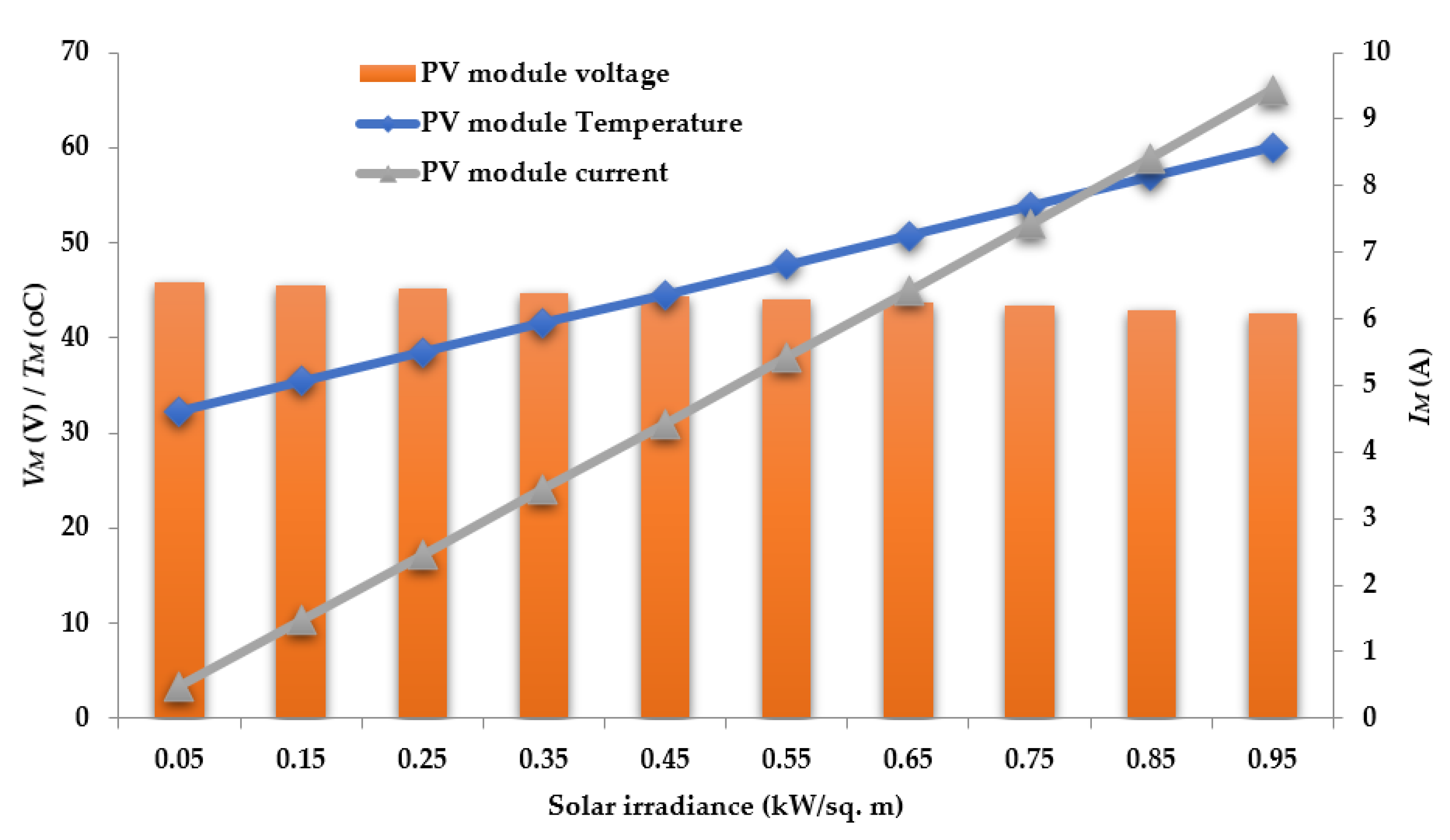
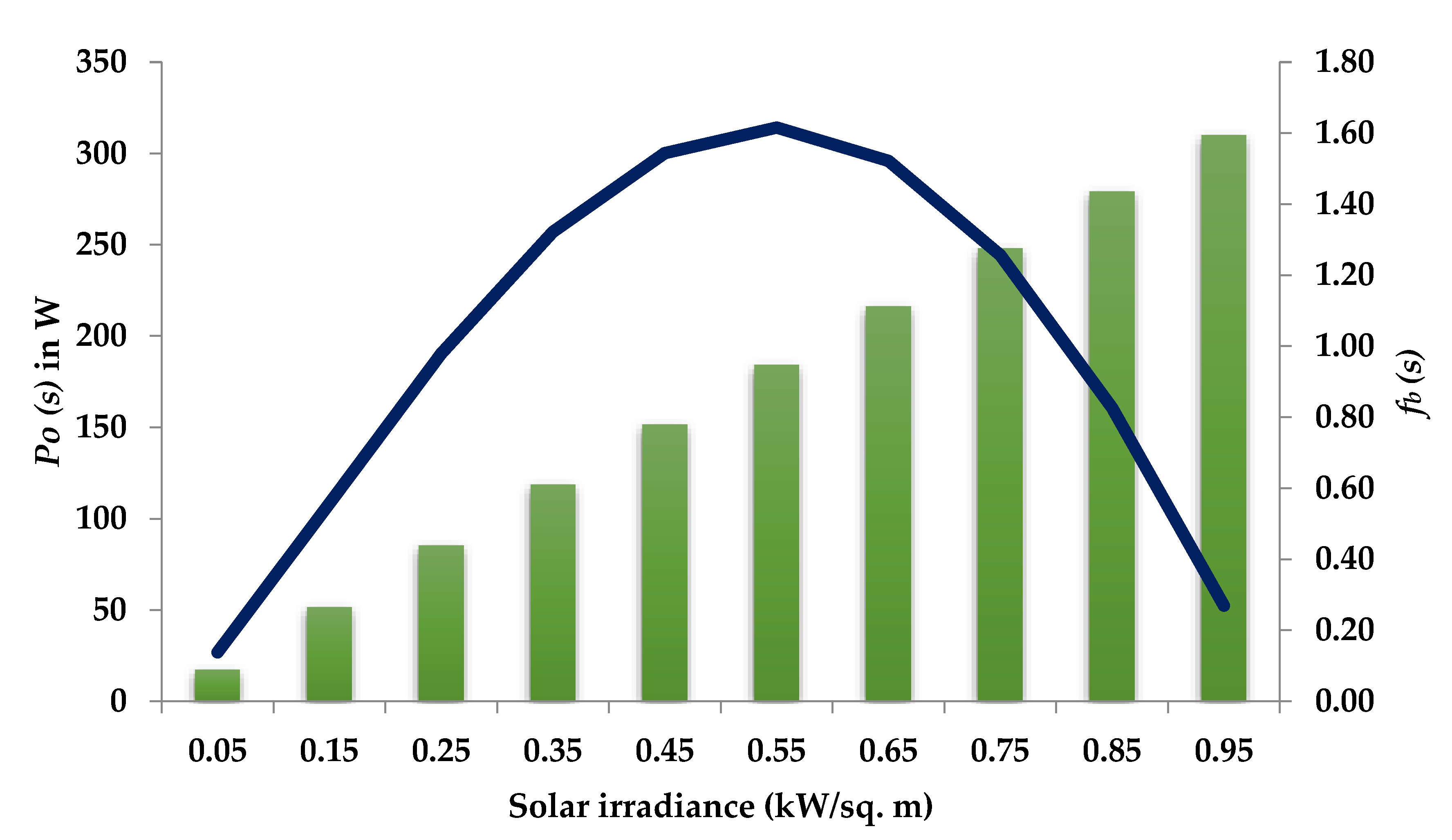
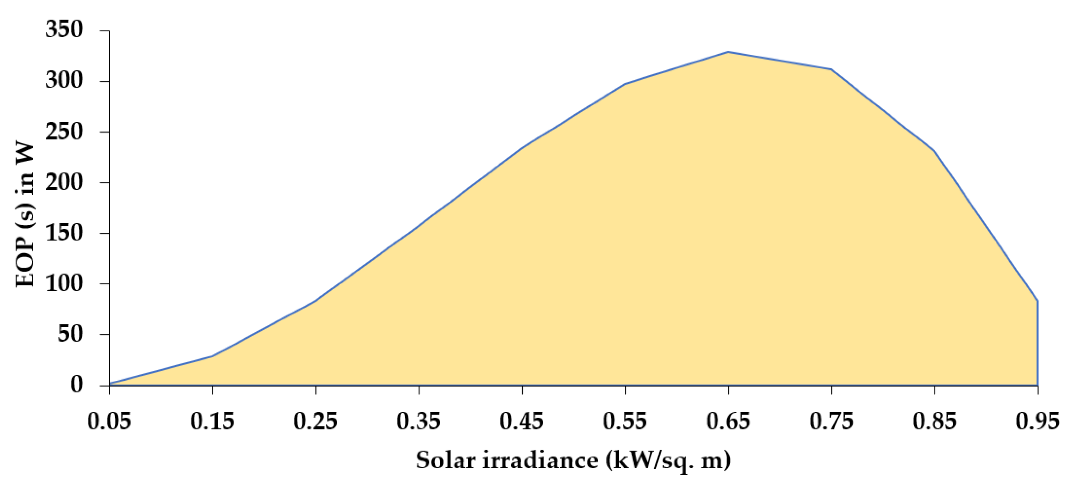
| Environmental Parameters | PV Module Parameters Considering Correction Factors | Modeling Parameters | Output | ||||
|---|---|---|---|---|---|---|---|
| s | |||||||
| 0.05 | 30.76 | 0.49 | 45.85 | 2.16 | 0.14 | 17.26 | 2.38 |
| 0.15 | 30.76 | 1.47 | 45.49 | 2.16 | 0.56 | 51.48 | 28.66 |
| 0.25 | 30.76 | 2.45 | 45.13 | 2.16 | 0.98 | 85.28 | 83.44 |
| 0.35 | 30.76 | 3.44 | 44.77 | 2.16 | 1.32 | 118.66 | 156.88 |
| 0.45 | 30.76 | 4.43 | 44.41 | 2.16 | 1.54 | 151.62 | 234.05 |
| 0.55 | 30.76 | 5.42 | 44.05 | 2.16 | 1.62 | 184.16 | 297.55 |
| 0.65 | 30.76 | 6.42 | 43.70 | 2.16 | 1.52 | 216.27 | 329.15 |
| 0.75 | 30.76 | 7.42 | 43.34 | 2.16 | 1.26 | 247.95 | 311.49 |
| 0.85 | 30.76 | 8.42 | 42.98 | 2.16 | 0.83 | 279.20 | 230.65 |
| 0.95 | 30.76 | 9.43 | 42.62 | 2.16 | 0.27 | 310.02 | 83.51 |
| Average | 175.78 | ||||||
| Type | ID | Functions | Fi = Fi(x) |
|---|---|---|---|
| Unimodal | F1 | Rotated High Conditioned Elliptic | 100 |
| F2 | Rotated Bent Cigar | 200 | |
| Simple Multimodal | F3 | Shifted and Rotated Rastrigin’s | 900 |
| F4 | Shifted Schwefel’s | 1000 | |
| Hybrid | F5 | Hybrid Function 3 (N = 4) | 1900 |
| F6 | Hybrid Function 4 (N = 4) | 2000 | |
| Composition | F7 | Composition Function 8 (N = 3) | 3000 |
| ID | Parameters | PSO | TLBO | CS | GSA | SFS | HHO |
|---|---|---|---|---|---|---|---|
| F1 | max | 4.56 × 10⁸ | 8.93 × 10⁸ | 5.51 × 10⁸ | 5.31 × 10⁷ | 1.17 × 10⁶ | 3.01 × 10⁵ |
| min | 2.47 × 10⁸ | 4.39 × 10⁷ | 1.18 × 10⁸ | 4.56 × 10⁶ | 1.54 × 10⁵ | 1.43 × 10⁴ | |
| median | 3.31 × 10⁸ | 3.42 × 10⁸ | 3.10 × 10⁸ | 8.37 × 10⁶ | 6.16 × 10⁵ | 1.52 × 10⁵ | |
| std | 7.92 × 10⁷ | 3.42 × 10⁸ | 1.05 × 10⁸ | 1.32 × 10⁷ | 2.35 × 10⁵ | 1.23 × 10⁵ | |
| F2 | max | 3.63 × 10¹⁰ | 4.06 × 10⁴ | 2.42 × 10⁴ | 1.61 × 10⁴ | 2.00 × 10² | 2.00 × 10² |
| min | 6.00 × 10⁷ | 6.00 × 10³ | 3.09 × 10² | 3.47 × 10³ | 2.00 × 10² | 2.00 × 10² | |
| median | 1.55 × 10¹⁰ | 1.52 × 10⁴ | 8.08 × 10³ | 8.38 × 10³ | 2.00 × 10² | 2.00 × 10² | |
| std | 1.43 × 10¹⁰ | 8.65 × 10³ | 6.00 × 10³ | 2.90 × 10³ | 7.89 × 10⁻⁹ | 0. 00 | |
| F3 | max | 1.24 × 10³ | 1.12 × 10³ | 1.34 × 10³ | 1.10 × 10³ | 9.84 × 10² | 9.03 × 10² |
| min | 1.13 × 10³ | 1.06 × 10³ | 1.15 × 10³ | 1.02 × 10³ | 9.35 × 10² | 9.20 × 10² | |
| median | 1.18 × 10³ | 1.09 × 10³ | 1.25 × 10³ | 1.06 × 10³ | 9.61 × 10² | 9.19 × 10² | |
| std | 4.33 × 10 | 0.25 × 10² | 4.41 × 10 | 1.74 × 10 | 1.11 × 10 | 1.017 × 10 | |
| F4 | max | 7.90 × 10³ | 5.92 × 10³ | 3.21 × 10³ | 5.25 × 10³ | 2.71 × 10³ | 1.05 × 10³ |
| min | 6.26 × 10³ | 4.14 × 10³ | 1.36 × 10³ | 3.45 × 10³ | 1.02 × 10³ | 1.00 × 10³ | |
| median | 7.18 × 10³ | 5.06 × 10³ | 2.17 × 10³ | 4.37 × 10³ | 1.49 × 10³ | 1.01 × 10³ | |
| std | 5.98 × 10² | 7.89 × 10² | 4.33 × 10² | 3.61 × 10² | 3.62 × 10² | 1.45 × 10 | |
| F5 | max | 2.10 × 10³ | 1.91 × 10³ | 2.04 × 10³ | 2.00 × 10³ | 1.91 × 10³ | 1.92 × 10³ |
| min | 1.91 × 10³ | 1.90 × 10³ | 1.91 × 10³ | 1.91 × 10³ | 1.90 × 10³ | 1.90 × 10³ | |
| median | 1.97 × 10³ | 1.91 × 10³ | 1.92 × 10³ | 2.00 × 10³ | 1.91 × 10³ | 1.91 × 10³ | |
| std | 7.07 × 10 | 1.65 | 3.30 × 10 | 3.43 × 10 | 1.47 | 1.46 | |
| F6 | max | 4.37 × 10³ | 5.34 × 10³ | 6.02 × 10⁴ | 6.82 × 10⁴ | 2.10 × 10³ | 2.75 × 10³ |
| min | 2.55 × 10³ | 2.30 × 10³ | 2.22 × 10⁴ | 2.32 × 10³ | 2.02 × 10³ | 2.00 × 10³ | |
| median | 3.00 × 10³ | 2.74 × 10³ | 3.68 × 10⁴ | 1.77 × 10⁴ | 2.06 × 10³ | 2.26 × 10³ | |
| std | 5.32 × 10² | 7.00 × 10² | 8.42 × 10⁴ | 1.39 × 10⁴ | 2.60 × 10 | 2.06 × 10² | |
| F7 | max | 9.70 × 10⁵ | 1.56 × 10⁶ | 5.08 × 10⁵ | 1.14 × 10⁵ | 7.66 × 10³ | 5.62 × 10³ |
| min | 6.90 × 10⁴ | 2.08 × 10⁴ | 6.26 × 10⁴ | 1.22 × 10⁴ | 4.25 × 10³ | 3.56 × 10³ | |
| median | 3.35 × 10⁵ | 6.56 × 10⁵ | 1.77 × 10⁵ | 1.46 × 10⁴ | 5.63 × 10³ | 4.71 × 10³ | |
| std | 3.63 × 10⁵ | 5.64 × 10⁵ | 9.11 × 10⁴ | 1.84 × 10⁴ | 7.38 × 10² | 1.30 × 10³ |
| Test System | Buses Count | Array Location | Ploss (kW) | Loss Reduction (%) |
|---|---|---|---|---|
| 33 bus system | 1 | 30 | 129.20 | 38.76 |
| 2 | 12, 30 | 86.90 | 58.81 | |
| 3 | 13, 24, 30 | 72.10 | 64.42 |
| Optimization Method | Bus Count | Array Location | DG Size (MW) | Total DG Size (MW) | Ploss (kW) | Loss Reduction (%) |
|---|---|---|---|---|---|---|
| Base case | - | - | - | - | 202.67 | 0.00 |
| TLBO [68] | 3 | 12 | 1.1826 | 3.560 | 124.70 | 38.47 |
| 28 | 1.1913 | |||||
| 30 | 1.1863 | |||||
| GA [69] | 3 | 11 | 1.5000 | 2.994 | 106.30 | 47.55 |
| 29 | 0.4230 | |||||
| 30 | 1.0710 | |||||
| PSO [69] | 3 | 8 | 1.1770 | 2.989 | 105.30 | 48.04 |
| 13 | 0.9820 | |||||
| 32 | 0.8300 | |||||
| GA/PSO [69] | 3 | 11 | 0.9250 | 2.998 | 103.40 | 48.98 |
| 16 | 0.8630 | |||||
| 32 | 1.2000 | |||||
| QOTLBO [68] | 3 | 13 | 1.0834 | 3.470 | 103.40 | 48.98 |
| 26 | 1.1876 | |||||
| 30 | 1.1992 | |||||
| CTLBO ε-method [70] | 3 | 13 | 1.1926 | 3.693 | 96.17 | 52.55 |
| 25 | 0.8706 | |||||
| 30 | 1.6296 | |||||
| IMOEHO [71] | 3 | 14 | 1.0570 | 3.852 | 95.00 | 53.13 |
| 24 | 1.0540 | |||||
| 30 | 1.7410 | |||||
| I-DBEA [72] | 3 | 13 | 1.0980 | 3.913 | 94.85 | 53.20 |
| 24 | 1.0970 | |||||
| 30 | 1.7150 | |||||
| CTLBO [70] | 3 | 13 | 1.0364 | 3.721 | 85.96 | 57.59 |
| 24 | 1.1630 | |||||
| 30 | 1.5217 | |||||
| BA [39] | 3 | 15 | 0.81630 | 2.721 | 75.05 | 62.97 |
| 25 | 0.95235 | |||||
| 30 | 0.95235 | |||||
| HHO [Proposed] | 3 | 13 | 0.8311 | 2.731 | 72.10 | 64.42 |
| 24 | 0.9500 | |||||
| 30 | 0.9500 |
| Test System | Bus Count | Array Location | DG Size (MW) | Ploss (kW) | Loss Reduction (%) |
|---|---|---|---|---|---|
| 69 bus system | 1 | 61 | 0.95 | 115 | 48.866 |
| 2 | 61, 62 | 0.95, 0.9118 | 83.4 | 62.916 | |
| 3 | 17, 61, 62 | 0.5329, 0.95, 0.822 | 71.8 | 68.074 |
| Optimization Method | Bus Count | Array Location | DG Size (MW) | Total DG Size (MW) | Ploss (kW) | Loss Reduction (%) |
|---|---|---|---|---|---|---|
| Base case | - | - | - | - | 224.9 | 0.00 |
| GA [69] | 3 | 21 | 0.9297 | 2.9897 | 89 | 60.43 |
| 62 | 1.0752 | |||||
| 64 | 0.9848 | |||||
| PSO [69] | 3 | 61 | 1.1998 | 2.9879 | 83.2 | 60.43 |
| 63 | 0.7956 | |||||
| 17 | 0.9925 | |||||
| TLBO [68] | 3 | 13 | 1.0134 | 3.1636 | 82.172 | 63.46 |
| 61 | 0.9901 | |||||
| 62 | 1.1601 | |||||
| GA/PSO [69] | 3 | 63 | 0.8849 | 2.988 | 81.1 | 63.94 |
| 61 | 1.1926 | |||||
| 21 | 0.9105 | |||||
| QOTLBO [68] | 3 | 15 | 0.8114 | 2.9606 | 80.585 | 64.17 |
| 61 | 1.1470 | |||||
| 63 | 1.0022 | |||||
| CTLBO ε-method [70] | 3 | 12 | 0.9658 | 3.3301 | 79.66 | 64.58 |
| 25 | 0.2307 | |||||
| 61 | 2.1336 | |||||
| I-DBEA [72] | 3 | 61 | 2.1487 | 3.32 | 78.347 | 65.16 |
| 19 | 0.4717 | |||||
| 11 | 0.7126 | |||||
| SA [74] | 3 | 18 | 0.4204 | 2.1813 | 77.09 | 65.72 |
| 60 | 1.3311 | |||||
| 65 | 0.4298 | |||||
| CTLBO [70] | 3 | 11 | 0.5603 | 3.1411 | 76.372 | 66.04 |
| 18 | 0.4274 | |||||
| 61 | 2.1534 | |||||
| IWO [75] | 3 | 27 | 0.2381 | 1.9981 | 76.12 | 66.15 |
| 65 | 0.4334 | |||||
| 61 | 1.3266 | |||||
| BFOA [76] | 3 | 27 | 0.2954 | 2.0881 | 75.21 | 66.56 |
| 65 | 0.4476 | |||||
| 61 | 1.3451 | |||||
| MFO [77] | 3 | 61 | 2.0000 | 2.9625 | 72.37 | 67.82 |
| 18 | 0.3803 | |||||
| 11 | 0.5822 | |||||
| HHO [Proposed] | 3 | 17 | 0.5329 | 2.3049 | 71.8 | 68.07 |
| 61 | 0.9500 | |||||
| 62 | 0.8220 |
| Case No. | Bus No. | Targeted Power to Be Injected (kW) | Actual Size of PV DG (kW) | DC Overload (kW) | Number of PV Modules |
|---|---|---|---|---|---|
| Case 2 | 13 | 831.0 | 1655.00 | 824.00 | 4728 |
| 24 | 950.0 | 1891.00 | 941.00 | 5404 | |
| 30 | 950.0 | 1891.00 | 941.00 | 5404 | |
| Case 3 | 17 | 532.9 | 1061.08 | 528.18 | 3032 |
| 61 | 950.0 | 1891.59 | 941.59 | 5405 | |
| 62 | 822.0 | 1636.73 | 814.73 | 4676 |
Publisher’s Note: MDPI stays neutral with regard to jurisdictional claims in published maps and institutional affiliations. |
© 2021 by the authors. Licensee MDPI, Basel, Switzerland. This article is an open access article distributed under the terms and conditions of the Creative Commons Attribution (CC BY) license (https://creativecommons.org/licenses/by/4.0/).
Share and Cite
Chakraborty, S.; Verma, S.; Salgotra, A.; Elavarasan, R.M.; Elangovan, D.; Mihet-Popa, L. Solar-Based DG Allocation Using Harris Hawks Optimization While Considering Practical Aspects. Energies 2021, 14, 5206. https://0-doi-org.brum.beds.ac.uk/10.3390/en14165206
Chakraborty S, Verma S, Salgotra A, Elavarasan RM, Elangovan D, Mihet-Popa L. Solar-Based DG Allocation Using Harris Hawks Optimization While Considering Practical Aspects. Energies. 2021; 14(16):5206. https://0-doi-org.brum.beds.ac.uk/10.3390/en14165206
Chicago/Turabian StyleChakraborty, Suprava, Sumit Verma, Aprajita Salgotra, Rajvikram Madurai Elavarasan, Devaraj Elangovan, and Lucian Mihet-Popa. 2021. "Solar-Based DG Allocation Using Harris Hawks Optimization While Considering Practical Aspects" Energies 14, no. 16: 5206. https://0-doi-org.brum.beds.ac.uk/10.3390/en14165206