
Mechanism of Splitting Failure for High Sidewall Cavern of Hydropower Station Based on Complex Function and Strain Gradient


1
Research Center of Geotechnical and Structural Engineering, Shandong University, Jinan 250100, China
2
School of Qilu Transportation, Shandong University, Jinan 250002, China
*
Author to whom correspondence should be addressed.
Energies 2021, 14(18), 5870; https://0-doi-org.brum.beds.ac.uk/10.3390/en14185870
Submission received: 29 June 2021
/
Revised: 25 August 2021
/
Accepted: 14 September 2021
/
Published: 16 September 2021
Abstract
:With the rapid development of society, the number of hydropower projects has increased. During the construction of these projects, due to excavation-induced unloading, the high sidewalls of the hydropower station are often subject to splitting failure, which produces many adverse effects on the construction of the cavern. In order to reveal the formation mechanism of splitting failure of hydropower stations, based on the strain gradient theory and elasto-plastic damage theory, we proposed an elasto-plastic damage softening model. Using the ODE45 program in MATLAB, we solved the numerical solution of displacement and stress of circular cavern based on our proposed elastoplastic damage model. Then, we apply the complex function method and use the Schwarz–Christoffel integral formula to obtain the mapping function from the outer domain of the high sidewall cavern to the outer domain of the unit circle. Finally, the elastic-plastic region and displacement distribution of the high sidewall cavern are obtained by mapping the obtained elastic-plastic solution of the circular cavern under the axisymmetric condition. In future research, it is necessary to further study the corresponding relationship between the internal length parameter of the material and its internal microstructure in order to accurately determine the internal length parameter.
1. Introduction and Background
With the rapid development of society, people’s demand for electric energy is increasing, so there are a greater number of hydropower projects. However, with an increase in hydropower projects, it was discovered that some nonlinear deformations and failures occurred in the surrounding rock of caverns during the construction of these projects. These deformations and damages are a serious threat to the construction safety and long-term stability of underground caverns. Among them, the deformation failure mode of the splitting failure of the hydropower projects with a high sidewall is quite different from that of the shallow cavern, showing obvious discontinuity and nonlinear behavior. This splitting failure has been widely recorded and described by many researchers [1,2,3,4], as shown in Figure 1. However, there is no clear understanding of the formation mechanism of splitting failure of high sidewall cavern, and the traditional continuum mechanics theory cannot provide a satisfactory explanation.
Because the failure process of the rock is very complicated, it is difficult to obtain the ideal result if only the classical continuity mechanics method is used to describe it. Therefore, it is necessary to introduce the damage mechanics method in the study of splitting failure of high-side caverns of hydropower stations. Damage mechanics can well simulate the nonlinear behavior of rocks after the peak. In addition, it shows good applicability in simulating the strain-softening characteristics of rocks. Li et al. [5] applied elastic damage mechanics to model the softening behavior of rock masses. Then, they proposed a numerical method based on the maximum tensile stress criterion and strain energy density theory to simulate the zonal fracture phenomenon. Tao et al. [6] applied a damage formulation to simulate softening and modulus reduction to propose a new method to understand the mechanisms and behaviors of high initial stress rocks. Jia et al. [7] studied the damage evolution around deep underground openings under multiaxial stress through 3D numerical tests. The results showed that biaxial stress parallel to the free surface constrained by zero or low confinement stress contributes to spalling or parallel fracture of the slab.
In the compression test of rocks, as the load increases, the internal stress of the rock will rapidly decrease to a lower level after reaching its peak strength, showing obvious post-peak strain softening. At the same time, along with the decline in the bearing capacity of the rock, the deformation and failure of the rocks are also concentrated in one or several narrow-banded areas, which is the phenomenon of localization of the rock strain. In the experimental research on the strain localization of rocks, many scholars [8,9,10,11,12] have given strong evidence that there is an obvious strain gradient effect in the deformation localization zone, and the strain gradient effect plays a controlling role in the localized deformation and failure process of the rock. Fleck et al. [13,14,15,16,17,18,19] carried out a large number of studies related to strain gradient. Based on the concepts of statistical storage and geometric asymmetric dislocation, they introduced plasticity into the strain gradient theory and established a phenomenological strain gradient plasticity theory. Menzel et al. [20] Established geometric linear formulas for high-order gradient plasticity of single crystal and polycrystalline materials based on dislocation and incompatible continuum theory. They found that due to dislocations or incompatible stresses, higher-order strain gradients are introduced into the yield conditions, which is similar to the structure of motion hardening in form, so the back stress follows the law of nonlocal evolution. Therefore, if the strain gradient effect is ignored in the post-peak localized deformation and failure analysis of rocks, it will cause serious deviations between the analysis results and the real situation. Therefore, it is very important to introduce strain gradient theory into the study of splitting failure of hydropower station caverns.
The common tunnel section shape of an underground powerhouse of a hydropower station is not circular, but high sidewall. For non-circular caverns, the commonly used method is to equivalent them to circles with the same area for analysis, but results obtained in this way will produce large errors. In order to reduce the error, some experts and scholars introduce the complex function theory into the study of solving the analytical solutions of stress and displacement of underground non-circular caverns. In order to reduce the error, some scholars [21,22,23,24] have introduced the theory of complex variable function to solve the analytical solution of the stress and displacement of underground non-circular caverns. Deng et al. [25] used the complex variable function solution method to derive the analytical solution of the stress and displacement of the surrounding rock of a highway tunnel of arbitrary shape under the action of supporting pressure and remote site stress, and solved the numerical solution by programming on the MATLAB platform. Lu et al. [26] used the conformal mapping method of the complex function theory to determine the optimal shape of the closed concrete support. Yang et al. [27] used complex variable function theory and a multipolar coordinate system to study the scattering problem of lining circular tunnels in an anisotropic half-space, and gave typical numerical simulation results of surface displacement amplitude under different anisotropic parameters.
Although great progress has been made in studying the microscopic mechanisms of rock specimens [28,29,30,31,32], laboratory or field experiments [33,34,35,36,37,38,39], and numerical simulations [40,41,42,43], so far, the theoretical method of splitting failure of surrounding rock of high side wall caverns under high ground stress is not perfect, and there is no theoretical explanation widely accepted by everyone. It is urgent to establish a more scientific mechanical model to reveal the formation mechanism of splitting failure.
2. Objectives
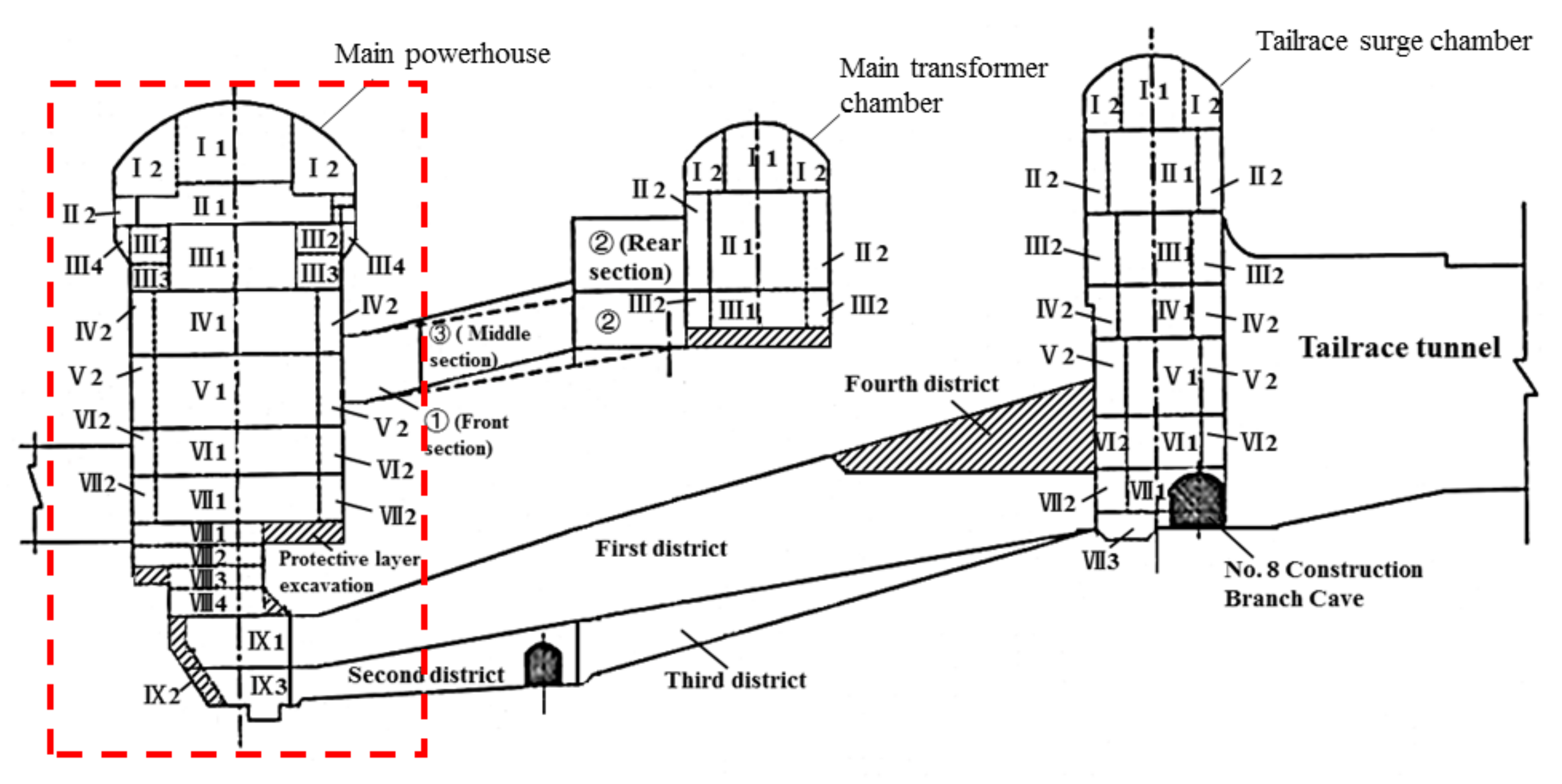
In this paper, we propose an elasto-plastic damage softening model based on strain gradient theory and elasto-plastic damage theory. Based on this elasto-plastic damage model, the numerical solutions for the displacements and stresses in the circular cavern were solved using the ODE45 program in MATLAB. Then, we applied the complex function method and use the Schwarz–Christoffel integral formula to obtain the mapping function from the outer domain of the high sidewall cavern to the outer domain of the unit circle. Next, the elasto-plastic solution conformal mapping of the circular cavern under axisymmetric conditions is used to obtain the elasto-plastic area and displacement distribution of the cavern with a high sidewall. Taking Pubugou Hydropower Station (Figure 2) as the engineering background, during the construction of the main powerhouse, several splitting cracks appeared on the sidewall, which caused the cracking of the concrete shotcrete on the sidewall. The maximum crack width was 20 mm. The numerical analysis results are basically consistent with the on-site monitoring and model test results. Finally, the variation of tangential stress of high side wall caverns with different height span ratios is obtained by comparison, which provides a theoretical basis for the study of the formation mechanism of splitting failure.
3. Establishment of Constitutive Model
3.1. Virtual Working Principle and Control Equation
In the Toupin–Mindlin strain gradient theory, in addition to the conventional strain tensor and stress tensor , higher-order strain terms and higher-order stress tensors that describe the state of the material are also required [11]. The expression of strain and its strain gradient term is:
Not only strain and higher-order strain terms are symmetric tensors, their corresponding stress and higher-order stress terms are also symmetric tensors. So, suppose that the strain rate and higher-order strain rate are both decomposed into elastic and plastic parts:
Similar to the strain gradient plasticity model proposed by previous scholars [17,20,44,45,46,47], it is assumed that the plastic higher-order strain term contributes to the work per unit volume. Since the principle of virtual work is divided into the work of elastic strain, the work of plastic strain, and the work carried out by their higher-order terms, the virtual work of its internal unit volume V can be expressed as:
where is called the micro stress tensor conjugated with plastic strain work; is the higher-order stress tensor conjugated to the plastic strain gradient work. Since the influence of and on virtual work are omitted in this paper, the above formula can be expressed as:
Using Gauss’s theorem to deal with the above formula, the following formula can be obtained:
where is the normal vector outward in the direction of the surface S. Since Equation (3) should be applied to any changes in plastic strain, and the second integral on the right side of Equation (5) disappears with any change, two sets of equilibrium equations can be determined:
According to the principle of virtual work, the corresponding conventional and high-order boundary conditions are obtained.
3.2. The Establishment of the Yield Function
For materials that exhibit plasticity, the stress state reaches a certain yield condition before it can enter the plastic state. The yield condition can be expressed by independent stress components and hardening parameters:
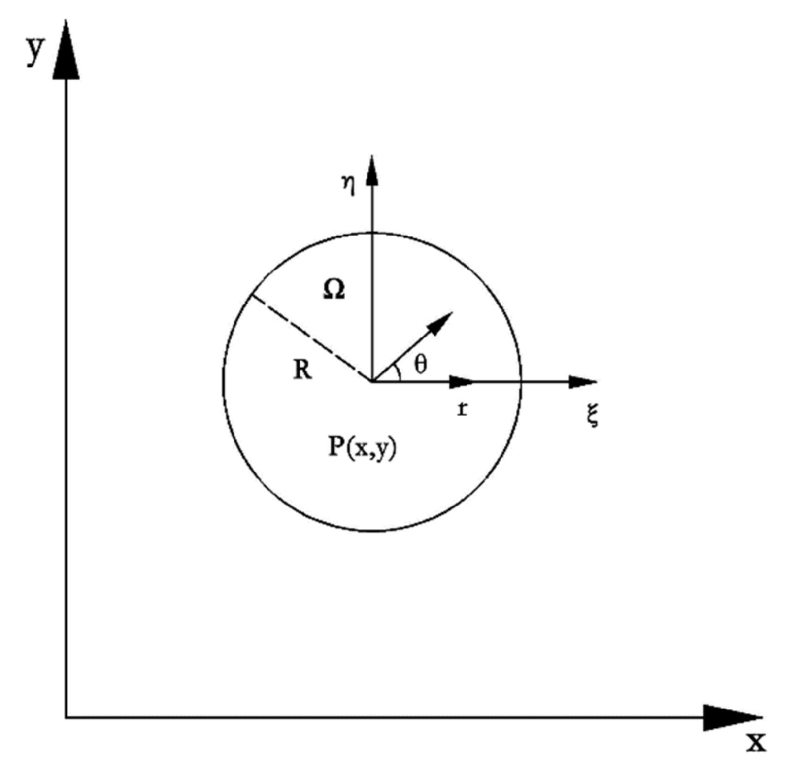
where H is the hardening parameter, which represents the relationship between yield stress and plastic deformation. For the classical elastic-plastic theory, the yield of a point in the material depends on its stress state and hardening parameters; for the theory of plastic strain gradient, the yield of the point in the material is not only related to the stress state and hardening parameters of the point itself, but also the influence of the surrounding points on the hardening parameters. When considering the influence of surrounding points on hardening parameters, point P with coordinate in the overall coordinate system is selected, and the neighborhood with surrounding radius R is taken as the neighborhood affecting point P, and the distance from any point in the neighborhood to the point is r, as shown in Figure 3. In the local coordinate system, the rectangular coordinates and polar coordinates of point P are and , respectively. Therefore, it is necessary to define a weighted average of hardening parameters to represent the influence of each point in the influence area on point P. The expression of the weighted average is:
Among them, is the material weight function, and the expression is selected as:
where, R is the radius of influence, ; l is the internal length parameter of the material, reflecting the length of the internal microstructure of the material; is the influence coefficient, for two-dimensional plane problems ; C is the weight function parameter, ; r is the distance from any point in the neighborhood to that point. The weight function has the characteristics of a single point of decline and the nature of normalization:
Use the above weight function to weighted average the hardening parameters at a certain point:
From this, the h(x,y) value of the internal length parameter l of the material can be obtained, which is expressed as the interaction between the microstructures. In order to obtain h(x + ξ, y + η) worthy of specifically related expressions, perform Taylor expansion of h(x,y) at this point:
For isotropic materials, the odd-order term is 0 after integration, use to transform the polar coordinates and rectangular coordinates in the integration and then take the integration before two items get:
Simplify the above formula to obtain:
where C is a constant; is in Laplacian form, . Equation (14) can be understood as the hardening parameter expression considering the effect of strain gradient, and is used to replace in the yield function of the classical plastic theory. The plastic strain gradient is introduced as an internal variable into the yield function of classical plastic theory. Introduce the hardening parameter considering the gradient term into the yield function:
At the same time, in order to meet the constraints, the yield function should also satisfy the following formula:
From this, the yield function of the plastic strain gradient theory is derived as:
The hardening modulus is defined as:
For further calculation, establish a certain relationship between the hardening function and the plastic multiplier:
where α is a relational constant. Further collation can be obtained:
Let , and further obtain the yield function of the plastic strain gradient theory as:
In the plane problem, the strengthening parameter H can be expressed by the equivalent plastic strain , so the yield model including the strain gradient term can be obtained from the formula:
where reflects the influence of plastic strain gradient and material internal length parameters on the yield function; κ is the hardening modulus, . Based on the Drucker–Prager strength criterion, the following yield function f and plastic potential function g are constructed:
where J2 is the second invariant of stress deviation; and are intensity parameters, and their expressions are as follows:
where is the friction angle and is expansion angle. When and are equal, it is the associated flow law.
3.3. Constitutive Equation
According to the strain gradient shaping theory, it is necessary to consider introducing the high-order stress related to the strain increment into the dissipation work generated by the high-order strain in a thermodynamically consistent manner [47,48]. The key to constructing the plastic constitutive equation considering the strain gradient is to define the effective stress work conjugated with the effective plastic strain rate of the gradient enhancement to ensure the plastic work rate:
Since , can be defined as:
where L is the dissipative length parameter. Thus, can be defined as:
From this, the dissipative plastic micro-stress tensor and the dissipative plastic high-order stress tensor are obtained, respectively:
When there is damage in the material, the Helmholtz free energy function can be defined as the following form with the dissipation potential function according to the first law of thermodynamics:
where is fourth-order elastic tensor; is the sixth-order elastic strain gradient damage tensor, ; is fourth-order plastic damage tensor, ; G is the shear modulus, ; l is the internal length parameter closely related to the micro-cracks and micro-defects in the rocks, and is an inherent parameter of the material; is a Kronecker symbol; D is the modified damage variable, ; is the correction parameter of the damage variable; d is the damage variable. Generally speaking, there is no damage when a material is in elastic state, and damage begins to appear when it enters plastic state. So, we define the following expression of the damage evolution equation:
where is the threshold for damage initiation; and are two material parameters; is elastic tensor of the isotropic body, and its matrix expression is:
The plastic tensor can take the following form according to the incremental theory in the elastoplastic theory:
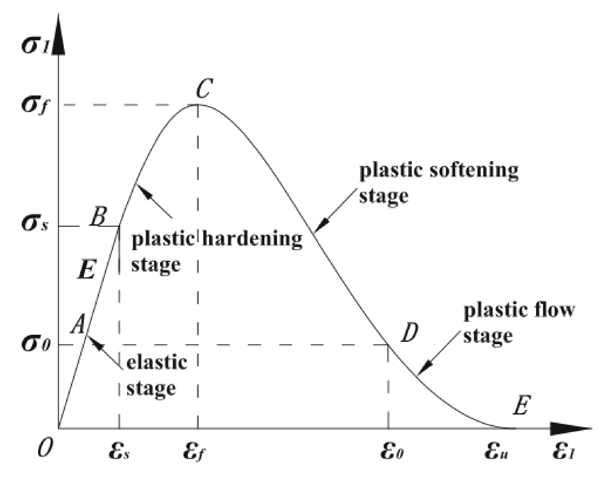
where H is the hardening function. Since rocks have both plastic hardening and plastic softening characteristics (Figure 4), its manifestation is defined as the following exponential form:
where ki (i = 1, 2, 3) is the material parameter; I1 is the first stress invariant representing the average stress or hydrostatic stress. The f and g in Equation (32) are the yield function and plastic potential function defined in Section 3.2, respectively.
The elastoplastic damage constitutive equation considering the strain gradient can be derived from the free energy function strain and strain gradient according to the second law of thermodynamics:
4. Obtained Mapping Function
4.1. Basic Assumption
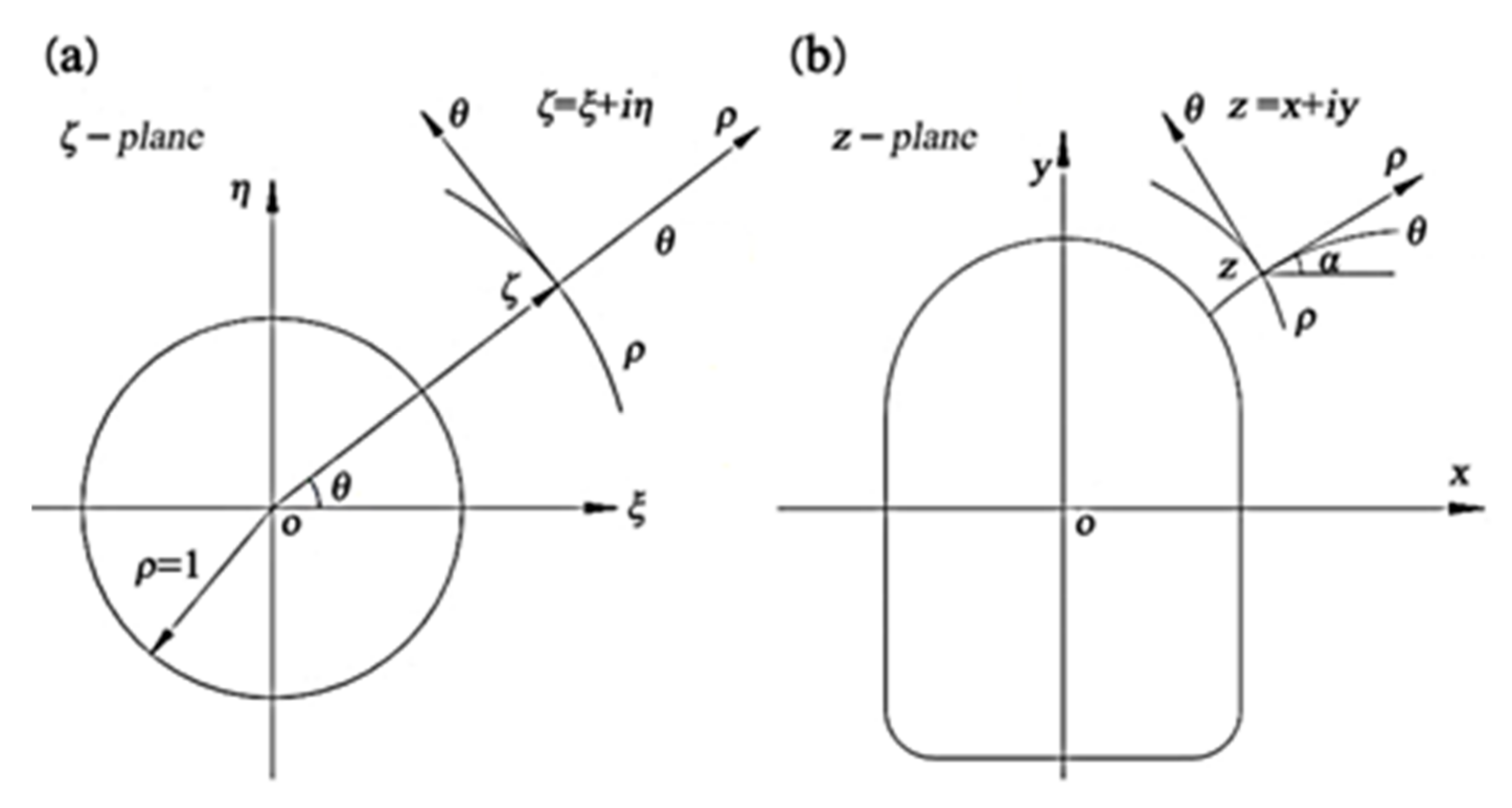
Some scholars [21,22,23,24,25,26,27] conducted preliminary research on the elastoplastic solution of non-circular caverns, including elastoplastic boundary and displacement field. Like these scholars, we apply the method of conformal function to solve the displacement and stress of the high side wall cavity. The specific steps are as follows: For the unit circular cavern with a radius of 1 in the physical z plane and the unit circle in the complex plane , the complex variable function method is used to conformally map the outer region of the circular cavern in the z plane to the outer region of the unit circle in the complex plane . In this case, the elastoplastic solution of the circular cavern in the physical plane z is the same as that of the unit circle in the complex plane . They extended it to non-circular caverns, and inversely mapped the plastic zone and displacement distribution on the complex plane to obtain the plastic zone and displacement distribution on the physical plane.
The result of conformal transformation is to change the singly connected domain to be discussed on the z-plane into the inside or outside of the unit circle centered on the origin on the complex plane , and the boundary line of this area is transformed into the circumference of the unit circle. The position of any point on the plane is expressed in polar coordinates as:
The coordinate lines are circumferential and radial. The circumferential line is represented by , and the radial line is represented by . The two are always orthogonal at each point (Figure 5). According to the nature of conformal transformation, the curves corresponding to the two groups of lines on the z-plane are also orthogonal. The curves on the two groups of z-planes can be regarded as the coordinate lines of the orthogonal curve coordinate system on the z-plane. So we also use and to sign, but the and lines on the z-plane are no longer circular and radial lines. Through the rectangular coordinate system and orthogonal curvilinear coordinate system, the coordinate transformation formulas of displacement and stress components between the rectangular coordinate system in the physical plane and polar coordinate system in the complex plane can be established.
4.2. Coordinate Transformation of Displacement Component
From Figure 5, it can be obtained that:
where is the angle between the axis and the x axis in the z plane; and are the displacements in x and y directions of a point in the cavern in the physical z plane, and and are the displacements in and directions of a point in the complex plane . The points in two different planes are connected by conformal mapping function:
It can be seen from the above formula that the corresponding relationship between the displacement components in two coordinate systems can be obtained only when is calculated. Since the and curve families on the z-plane are connected by the and curve families on the plane through , should start from this. Assuming that point B is given an infinitesimal increment dz along the axis on the z-plane, corresponding to the infinitely small increment of point A on the plane along the radial direction, then dz and are, respectively:
Because of , we can obtain:
Then, we can obtain the following results:
Therefore, the corresponding relationship between the rectangular coordinate system in the physical plane and the displacement component in the polar coordinate system in the complex plane is:
4.3. Coordinate Transformation of Stress Component
According to the axis formula in elastoplastic mechanics, the coordinate transformation formulas of the stress components in the following two different coordinate systems can be obtained:
It is obvious from the above equation that there is , and it follows that:
According to the previous expression of (Equation (25)), can be determined as:
Thus, the following corresponding relations of stress components in the two coordinate systems are obtained:
4.4. Approximate Solution of the Mapping Function
For high sidewall cavern, the mapping function from the outer domain of the cavern to the outer domain of the unit circle often takes the following form:
In the physical plane, the sidewall and bottom plate of the high sidewall cavern have a tendency to curve toward the inside of the cavern. That is, for the straight-line boundary part, when the number of mapping items is small, the boundary of the cavern determined by the mapping function is a curved edge. As the number of terms increases, the accuracy of the mapping becomes higher and higher, and the boundary of the cavity obtained by the mapping function gets closer to a straight line. Usually n = 4, that is, taking 5 terms has sufficient accuracy, so the integral function is taken as:
where, is a real constant, and there is a corresponding real constant a for hole shapes with different height span ratios ai, c. Based on the FORTRAN language, a mapping function parameter solving program was written according to the Schwarz–Christoffel formula. The parameters of the mapping function are shown in Table 1.
5. Numerical Results and Discussions
5.1. Basic Assumption
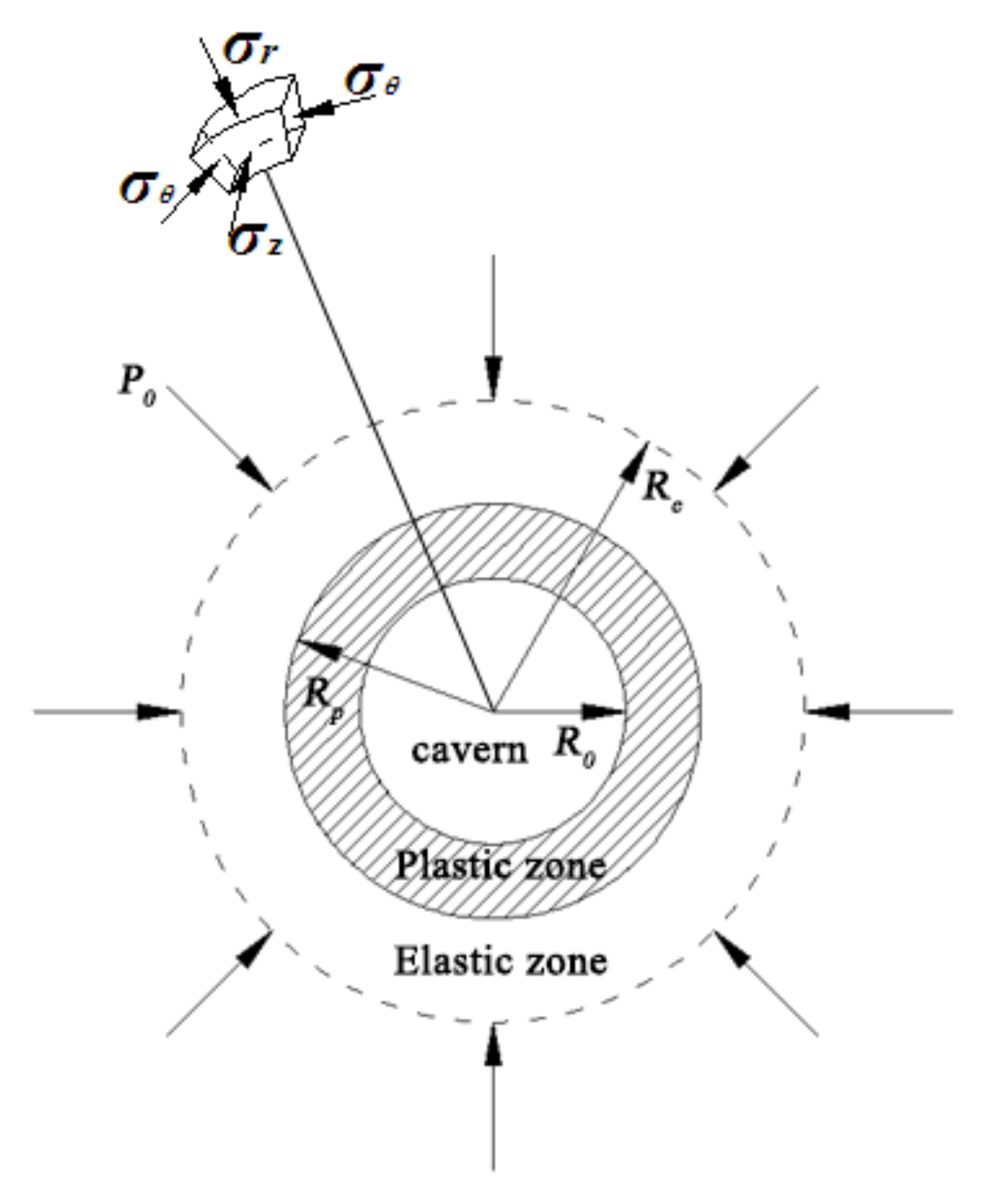
Considering the mechanical calculation model, when the length of the deep-buried horizontal cavern is large, it can be treated as a plane strain problem. Meanwhile, in classical elasto-plastic mechanics, a circular cavern under pressure and regardless of a body force is considered as a cylinder buried in an infinite elastoplastic body subjected to a uniform pressure q. Therefore, we define the following basic assumptions (Figure 6):
- is the radius of the circular cavern, is the radius of the plastic zone.
- The cavern is a deep buried cavern with infinite longitudinal length, and the uniform geostress is applied at the infinite distance of the cross section, regardless of body force.
- The surrounding rock of the cavern is isotropic elastic-plastic material.
- The compressive stress is positive and the tensile stress is negative.
5.2. Derivation of Balance Equation
Based on the basic assumptions, the cavern is an axisymmetric plane strain problem, ignoring body force. Due to the axial symmetry of the mechanical state of the surrounding rock of the deep cavern, it can be known that the displacement of any point in the surrounding rock is only a function of r, so the simplified geometric equation is:
According to the basic assumptions ignoring physical strength, the balance equation in the plane strain problem can be simplified to:
In the above equation, and are the generalized radial and tangential stresses in the surrounding rock after considering the higher order stress terms, respectively, and their expressions are as follows:
Substituting Equation (50) into Equation (49), the static equilibrium equation with higher-order stress terms can be obtained:
For the problem of thick-walled cylinders, the internal and external boundary conditions are:
where Tr and Rr are surface traction and high-order surface traction, respectively.
5.3. Derivation of Related Equations for Surrounding Rock of Deep Circular Cavern
The damage is not considered when the surrounding rock is in an elastic state. Combining the previous constitutive equations (Equations (34) and (35)) and the equilibrium equation (Equation (52)) together, the equilibrium equation for the elastic stage of the surrounding rock of the cavern can be obtained:
In order to solve the above-mentioned fourth-order ordinary differential equation and transform the higher-order ordinary differential equilibrium equation into a system of first-order differential equations, the following auxiliary variables need to be defined first:
The following expression can be obtained:
The corresponding coefficients in the above formula are: , , , . The boundary conditions at the boundary of the elastic zone () can also be obtained:
From the previously assumed yield function (Equation (16)), using the method of calculating the stress and displacement of the surrounding rock plastic zone used [49], we can obtain:
Then, the equation of the plastic damage state of the surrounding rock of the cavern can be obtained:
Substituting the previous static balance equation (Equation (36)) can obtain:
Define the same auxiliary variable as the elastic segment (Equation (56)), but the expression should be written as follows:
The corresponding coefficients in the above formula are: , , , , , , , , , , . The expressions of A, B and E are as follows:
The boundary conditions at the inner boundary () of the post peak strain softening zone can be obtained:
5.4. Solution Method for Displacement and Stress
The equilibrium equation (Equation (55)) in the elastic state and the equilibrium equation (Equation (61)) in the plastic damage state are both fourth-order ordinary differential equations (ODE), and the corresponding boundary conditions (Equation (57)) and (Equation (64)) are third-order ordinary differential equations. It is almost impossible to obtain analytical solutions to the above problems. Therefore, the numerical solutions of the above problems are solved by using MATLAB numerical analysis software.
The boundary conditions given in the above problems belong to boundary value problems at the inner and outer boundaries of surrounding rock; when the ODE45 function is used in MATLAB numerical analysis software, it should be first transformed into initial value problems. ODE45 is a special function for solving differential equations in MATLAB numerical analysis software, which adopts the fourth-fifth order Runge–Kutta algorithm. Its fourth-order algorithm provides candidate solutions, and the fifth-order algorithm controls errors. It is an adaptive step size numerical solution of ordinary differential equations and solves Nonstiff ordinary differential equations.
When applying the ODE45 function to solve high-order ordinary differential equations, it is necessary to provide initial solutions for calculation intervals and differential equations, and it is also necessary to convert high-order differential equations into first-order differential equations. The first-order differential equations transformed by higher-order differential equations have been given in the previous section. In order to solve the differential equation, it is still necessary to give the initial solution of the differential equation on the boundary. In the above problem, the surrounding rock in the range of A is in an elastic state. It is required to solve the fourth-order ordinary differential equation in the elastic zone (Equation (55)), and the initial solution on the outer boundary (Equation (58)) must be given, that is, the derivative values of each order of displacement at (, , and ).
From the calculation and analysis of Zhao et al. (2007), it can be seen that the displacement value obtained by applying two different theories (classical theory and strain gradient theory) in the elastic stage is not much different from its first derivative value. Therefore, the displacement value () and the displacement first derivative value () at E can be roughly estimated from the analytical solution of the thick-walled cylinder in the classical elastic theory, and then and are substituted into the boundary conditions (Equation (58)) to obtain and . In this way, the initial solution on the boundary required to solve the higher-order differential equation is obtained. The analytical solution of the thick-walled cylinder in the classical elastic theory is as follows:
In the above equation, E and are the elastic modulus and Poisson’s ratio of the surrounding rock respectively, a and b are the inner and outer diameters of the cylinder respectively, and and are the pressures on the inner and outer walls of the cylinder, respectively.
Due to the continuity of the deformation of the surrounding rock of the cavern, is both the inner boundary of the elastic zone and the outer boundary of the plastic damage zone, that is to say, the surrounding rock conforms to the equilibrium equation of the elastic zone (Equation (39)) and plastic damage zone (Equation (45)). Therefore, the following method is used to determine the size of : first, the calculation interval is set as ; combined with the initial values of the displacement derivatives , , and on the outer boundary of the elastic zone are estimated and determined; the ODE45 function in MATLAB is used to solve the differential equations (Equation (57)), and the numerical solution of each point in the range of can be obtained. According to the research of Gao et al. [8], find a point that satisfies the Equation (66), and the distance between this point and the center of the roadway is the size of .
After the boundary between the elastic zone and plastic damage zone is determined, the displacement derivatives (, , and ) on the inner boundary of the elastic zone can be calculated; it is taken as the initial value on the outer boundary of the plastic damage zone, and the calculation interval is set as ; the numerical solution (, , and ) of each point in the range of can be obtained by solving the differential equations (Equation (62)) with ODE45 function in MATLAB.
Take the derivative values of the displacements (, , and ) on the boundary of the plastic damage zone and substitute them into Equations (67) and (68) to check the calculation errors. This calculation error is caused by the estimated initial value (, , and ) on the outer boundary of the elastic zone. If the error meets the requirements (), the calculation ends to obtain the numerical solution of the entire calculation area; if the error does not meet the requirements (), adjust the initial value on the outer boundary of the elastic zone and repeat the above calculation steps until the error meets the requirements, and obtain the numerical solution of the entire calculation area. The calculation flowchart of the solution process is shown in Figure 7.
5.5. Analysis of Theoretical Calculation Results
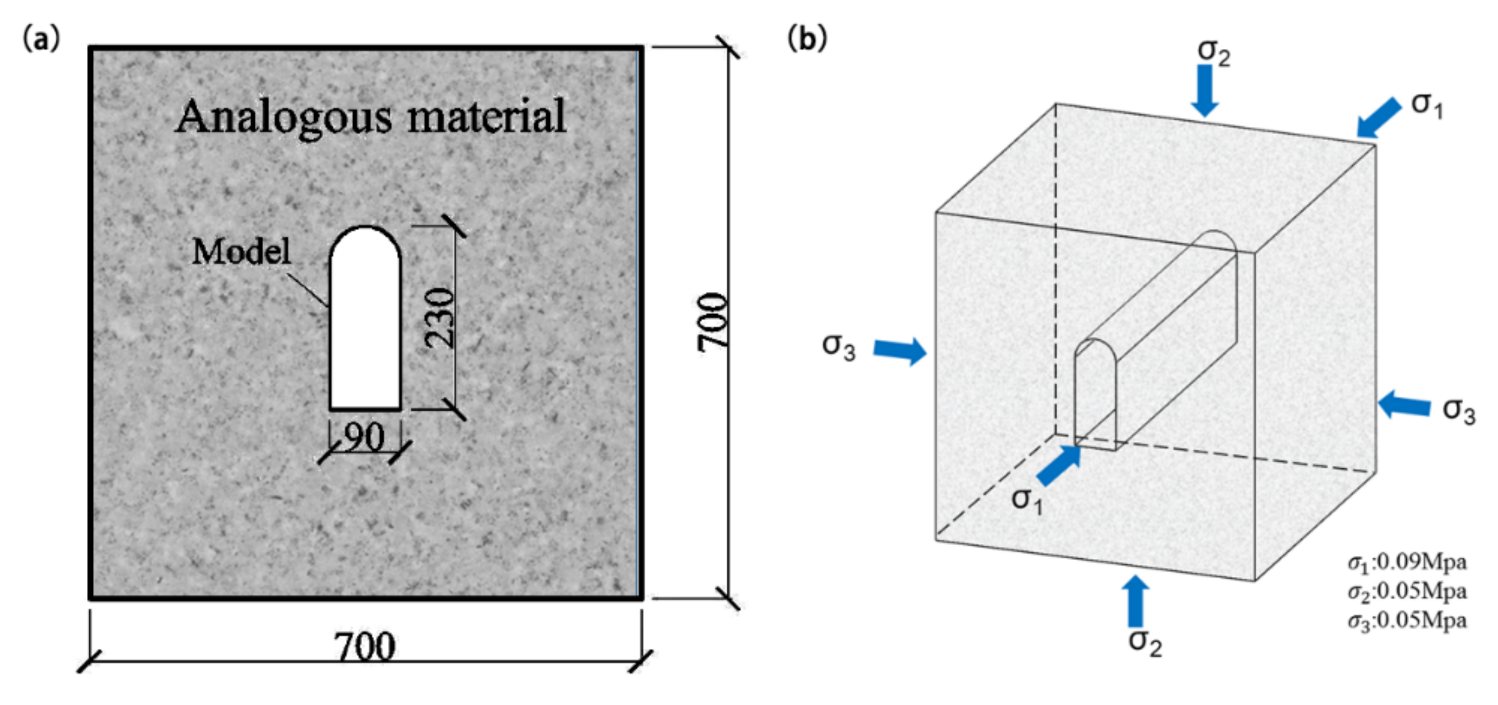
In this paper, the radial displacement, radial stress, and tangential stress distribution of the high sidewall cavern are obtained using rock parameters (Table 2) of the Pubugou Hydropower Station as calculation parameters. The top of the main powerhouse is 360 m from the ground surface and the cross-section size of the cavern cross-section is measures 26.8 m × 70.1 m. Then, the theoretical calculation results are compared and analyzed with the geomechanical model test results [50] to initially verify the applicability of the splitting failure elastic-plastic damage model in the study of splitting damage in a deep cavern. The geomechanical model test program and results are shown in Figure 8 and Figure 9, respectively.
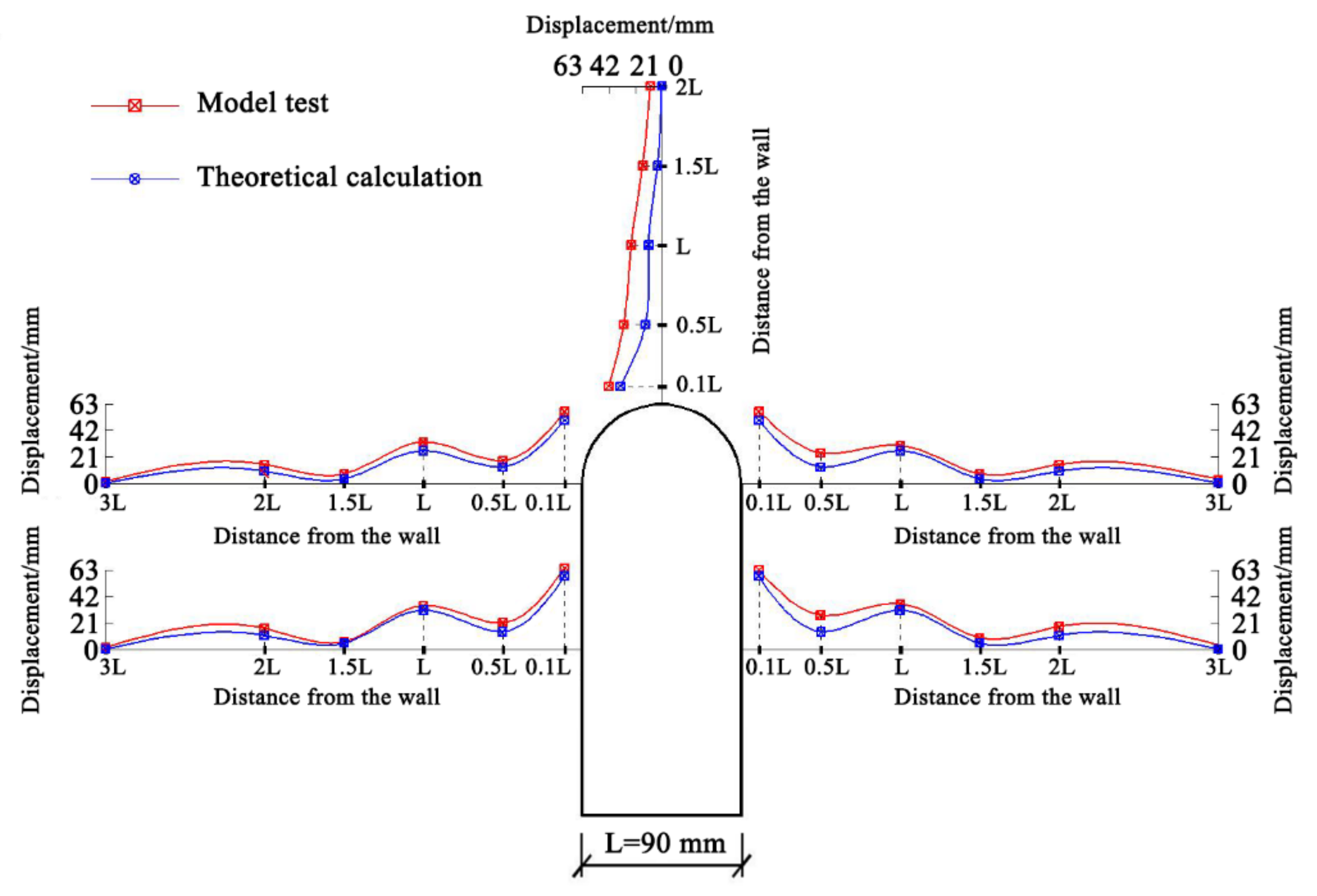
Using the above calculation parameters, the numerical solution of the radial displacement, radial stress, and tangential stress of the rock of the high sidewall cavern is calculated according to the solution process shown in Figure 7. In this section, in order to facilitate the comparison between theoretical calculation results and model test results, all model test results are converted into prototypes based on the principles of similitude. Figure 10 shows the radial displacement distribution diagram of the surrounding rock of the high sidewall cavern. The theoretically calculated values and experimentally measured values of the radial displacement, radial stress, and tangential stress at the corresponding positions of the measuring points around the cavern are listed in Table 3.
It can be seen from Figure 10 that the radial displacement at the high sidewall of the cavern obtained by using the elastic-plastic damage model of splitting failure shows an oscillating attenuation, and the oscillation amplitude gradually decreases with an increase in the distance from the sidewall, which is consistent with the variation measured by the model test. Because the theoretical model ignores the influence of excavation damage, the calculated displacement value is less than the displacement value of the model test. The difference close to the sidewall is as small as no more than 13%, and the value at the trough of the oscillating change is quite different, with the maximum difference being 12.66 mm. Comparing the measured values in Table 3 with the calculated values, it can be seen that they are very close in most positions. It is preliminarily confirmed that the elasto-plastic damage model of splitting failure is applicable to the study of splitting failure of high sidewall cavern.
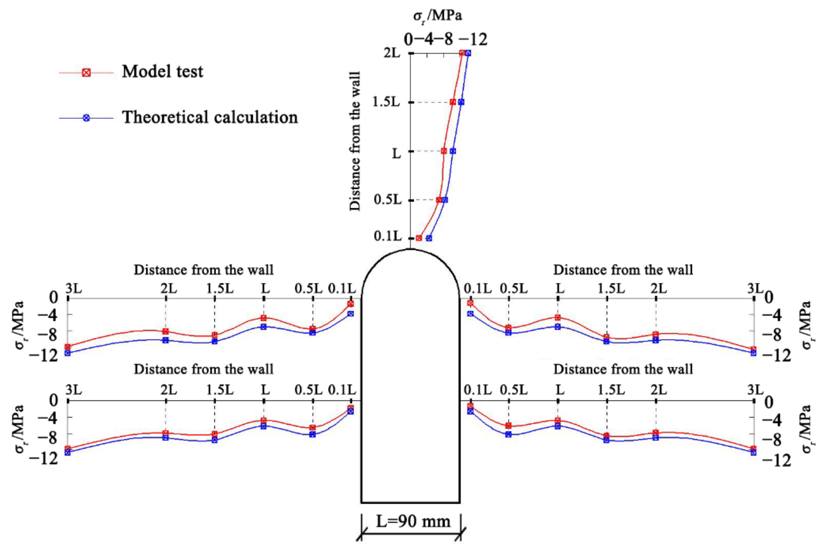
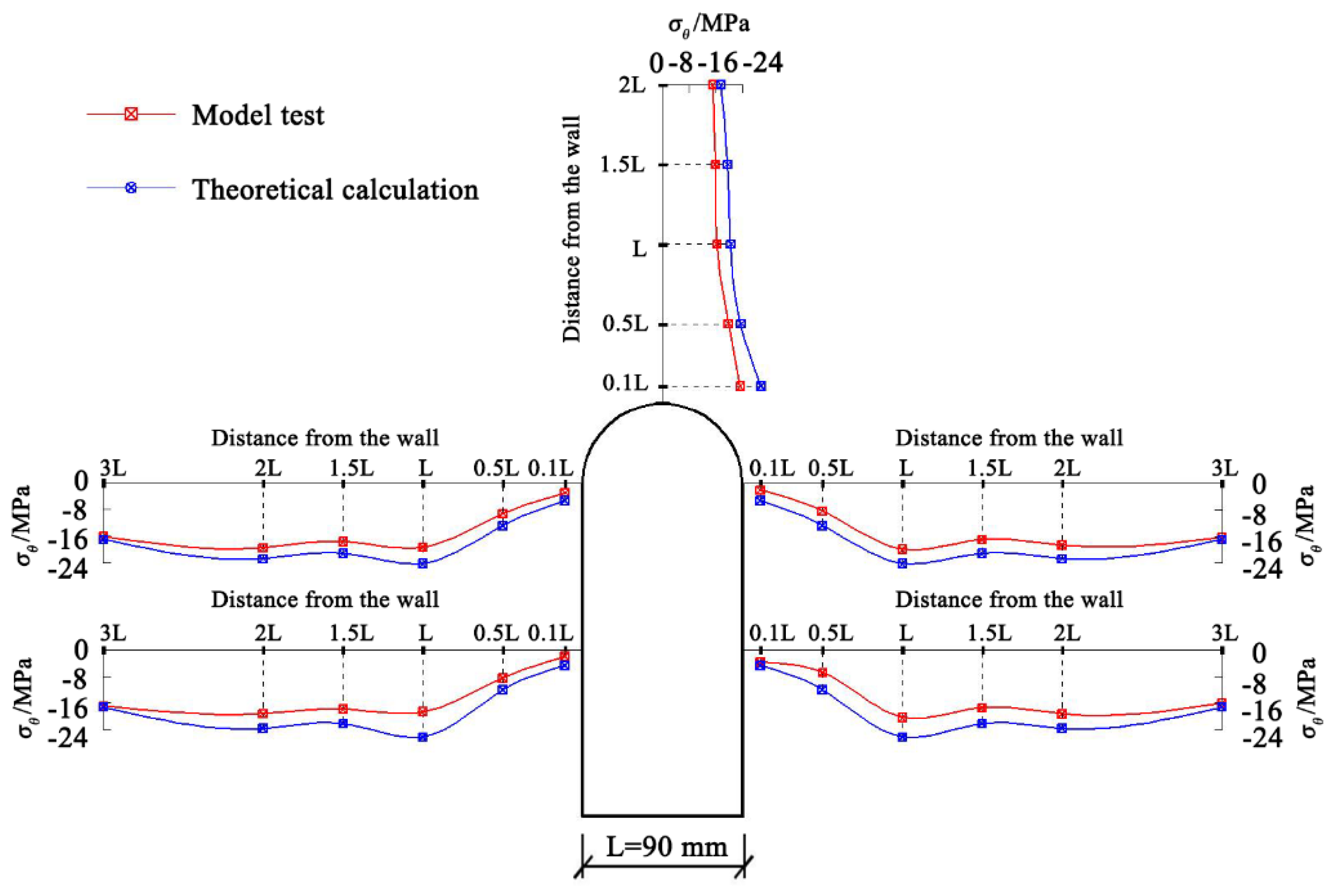
The stress distribution of rock of the high sidewall cavern was also obtained by using the splitting failure elastoplastic damage model, as shown in Figure 11 and Figure 12. Table 4 and Table 5 present the radial and tangential stresses of theoretical calculations and model tests, respectively. Figure 11 shows the comparison of the radial stress distribution between theoretical calculation and model test. We find that the distribution of radial stresses is similar to that of displacements. The calculated radial stress value is relatively close to the test monitoring result, and the maximum difference does not exceed 2 MPa. As shown in Figure 12, the theoretically calculated tangential stress distribution is also consistent with the model test. When the distance from the sidewall is less than L, the rock is in a plastic state and the tangential stress is released; when the distance from the sidewall is greater than L, the tangential stress is concentrated and the rock is in an elastic state. The tangential stresses at the vault are all greater than the in-suit value (σθ = 15.25 MPa). Due to ignoring the excavation disturbance, the calculated value of the tangential stress is generally greater than the test value. When the tangential stress just appears to be concentrated, the gap is large, and the maximum gap between the two is 28.83%.
The numerical solution of the radial displacement and radial stress of the surrounding rock of the high side wall cavern using the splitting failure elastoplastic damage softening model for theoretical calculations shows that the oscillation attenuation occurs alternately with wave crests and wave troughs. This is completely different from the monotonic attenuation obtained by using the classic continuous elastoplastic model and is consistent with the change rule obtained by the geomechanical model test. This indicates that the split failure elastoplastic damage model can explain the split failure of high side wall caverns under high ground stress conditions.
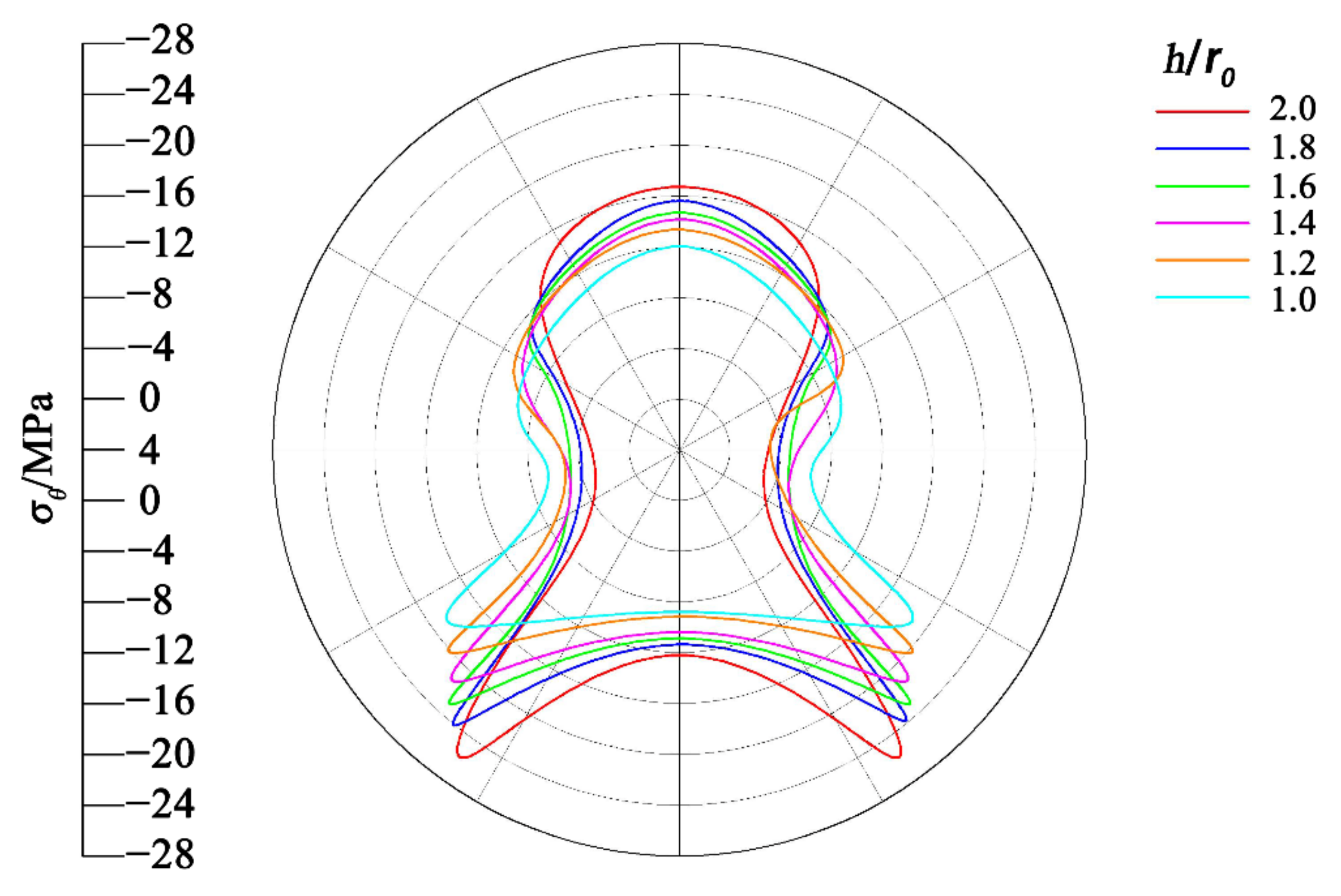
In order to study the formation mechanism of splitting failure of high sidewall caverns of hydropower stations, we compared the distribution of tangential stress around the high sidewall caverns under different height–span ratios, as shown in Figure 13. We find that the stress distribution of the surrounding rock of the high side wall cavern is significantly affected by the height–span ratio. The tangential stress is unevenly distributed along the boundary of the cavern and is symmetrically distributed along the central axis of the cavern. There are obvious stress fluctuations in surrounding rock near the vault, arch toe, and lower corner of the side wall. With an increase in the height–span ratio of the cavern, the tangential stress of the vault and the lower corner becomes larger and larger. The maximum tangential stress at the midpoint of the side wall shows a decreasing trend. The release of the tangential stress increases gradually, and the damage of the surrounding rock increases gradually.
6. Conclusions
Based on the strain gradient theory and continuum damage mechanics, the splitting failure elasto-plastic damage model is established. By using complex variable function mapping, the variations of radial displacement, radial stress, and tangential stress of surrounding rock of high sidewall cavern are obtained. The theoretical calculation results and model test results are compared and analyzed, and the following research conclusions are obtained:
- (1)
- A yield function with strain gradient is established, which can describe the plastic hardening and softening of quasi-brittle materials such as rock at the same time. Based on this, an elastic-plastic damage softening constitutive model considering strain gradient is established.
- (2)
- The calculation program is compiled by MATLAB software, and the variations of radial displacement, radial stress, and tangential stress of surrounding rock of circular cavern are calculated. Then, the variations of high side wall cavern under high ground stress are mapped by using the obtained mapping function.
- (3)
- The theoretical calculation value and the measured value of the model test are in good agreement in both the value and the variations, which confirms the applicability of the splitting failure elasto-plastic damage model.
- (4)
- Through comparison, the variations of tangential stress in high side wall caverns with different height–span ratios are obtained: as the height-to-span ratio of the cavern increases, the tangential stress release at the sidewall gradually increases, and the damage to the surrounding rock also gradually increases.
7. Recommendations for Future Research
In this paper, an elastoplastic damage softening constitutive model that can simultaneously describe the plastic hardening and softening processes of rock and other quasi-brittle materials considering the strain gradient is established. In addition, we use the model to calculate the displacement and stress values of the split failure of the high side wall cavity. Among them, the internal length parameter of the material is related to the internal microstructure of the rock material and is a key parameter in the strain gradient theory. At present, the method of determining the internal length parameters of materials by measuring the width of the shear band can only be applied to specific models and materials and does not have broad significance. Therefore, it is necessary to further study the corresponding relationship between the internal length parameters and their internal microstructure in order to accurately determine the internal length parameters.
Author Contributions
Conceptualization, Q.Z.; methodology, F.L.; software, F.L.; validation, F.L.; formal analysis, F.L.; investigation, F.L.; resources, F.L.; data curation, W.X.; writing—original draft preparation, F.L.; writing—review and editing, Q.Z.; visualization, W.X.; supervision, Q.Z.; project administration, W.X.; funding acquisition, Q.Z. All authors have read and agreed to the published version of the manuscript.
Funding
This research was funded by the Natural Science Foundation of China, grant number NO:41772282 and the Taishan Scholars Project Foundation of Shandong Province and the National Key Research Development Project of China, grant number No. 2016YFC0401804.
Institutional Review Board Statement
Not applicable.
Informed Consent Statement
Not applicable.
Conflicts of Interest
The authors declare no conflict of interest.
Nomenclature
| Euler strain tensor | |
| Cauchy stress tensor | |
| Higher-order strain terms | |
| Higher-order stress tensors | |
| Elastic strain tensor | |
| Plastic strain tensor | |
| Elastic higher-order strain terms | |
| Plastic higher-order strain terms | |
| Virtual work | |
| V | Internal unit volume |
| Micro stress tensor | |
| Normal vector | |
| Traction | |
| Higher-order external force | |
| Yield function | |
| H | Hardening parameter |
| Material weight function | |
| R | Radius |
| Influence coefficient | |
| l | Internal length parameter of the material |
| Constant | |
| κ | Hardening modulus |
| J2 | Second invariant of stress deviation |
| Equivalent plastic strain | |
| Friction angle | |
| Expansion angle | |
| Effective stress | |
| L | Dissipative length parameter |
| Dissipative plastic micro-stress tensor | |
| Dissipative plastic high-order stress tensor | |
| Fourth-order elastic tensor | |
| Sixth-order elastic strain gradient damage tensor | |
| Fourth-order plastic damage tensor | |
| G | Shear modulus |
| Kronecker symbol | |
| D | Modified damage variable |
| Correction parameter of the damage variable | |
| d | Damage variable |
| Fourth-order plastic tensor | |
| Complex plane | |
| z | Physical plane |
| Displacements | |
| Radius of the circular cavern | |
| Radius of the plastic zone | |
| Uniform geostress | |
| Generalized radial stresses | |
| Generalized tangential stresses | |
| Equivalent strain | |
| Yield strain | |
| Error vector | |
| Tolerance |
References
- Yoshida, T.; Ohnishi, Y.; Nishiyama, S.; Hirakawa, Y.; Mori, S. Behavior of discontinuties during excavation of two large underground caverns. Int. J. Rock Mech. Min. Sci. 2004, 41, 1–6. [Google Scholar] [CrossRef]
- Ortlepp, W.D.; Stacey, T.R. Rockburst mechanisms in tunnels and shafts. Tunn. Undergr. Sp. Technol. 1994, 9, 59–65. [Google Scholar] [CrossRef]
- Martin, C.D.; Maybee, W.G. The strength of hard-rock pillars. Int. J. Rock Mech. Min. Sci. 2000, 37, 1239–1246. [Google Scholar] [CrossRef]
- Hibino, S. Rock Mass Behavior of Large-scale Cavern during Excavation and Trend of Underground Space Use. Shigen-to-Sozai 2001, 117, 167–176. [Google Scholar] [CrossRef]
- Li, S.C.; Feng, X.D.; Li, S.C. Numerical model for the zonal disintegration of the rock mass around deep underground workings. Theor. Appl. Fract. Mech. 2013, 67, 65–73. [Google Scholar] [CrossRef]
- Tao, M.; Li, X.; Wu, C. 3D numerical model for dynamic loading-induced multiple fracture zones around underground cavity faces. Comput. Geotech. 2013, 54, 33–45. [Google Scholar] [CrossRef] [Green Version]
- Jia, P.; Yang, T.H.; Yu, Q.L. Mechanism of parallel fractures around deep underground excavations. Theor. Appl. Fract. Mech. 2012, 61, 57–65. [Google Scholar] [CrossRef]
- Gao, Q.; Zhang, Q.; Xiang, W. Mechanism of Zonal Disintegration Phenomenon (ZDP) Around Deep Roadway Under Dynamic Excavation. Geotech. Geol. Eng. 2019, 37, 25–41. [Google Scholar] [CrossRef]
- Zbib, H.M.; Aifantis, E.C. On the structure and width of shear bands. Scr. Metall. 1988, 22, 703–708. [Google Scholar] [CrossRef]
- Zbib, H.M.; Aifantis, E.C. A gradient-dependent model for the Portevin-Le Chatelier effect. Scr. Metall. 1988, 22, 1331–1336. [Google Scholar] [CrossRef]
- Zhang, Q.; Zhang, X.; Wang, Z.; Xiang, W.; Xue, J. Failure mechanism and numerical simulation of zonal disintegration around a deep tunnel under high stress. Int. J. Rock Mech. Min. Sci. 2017, 93, 344–355. [Google Scholar] [CrossRef]
- Steinmann, P. A micropolar theory of finite deformation and finite rotation multiplicative elastoplasticity. Int. J. Solids Struct. 1994, 31, 1063–1084. [Google Scholar] [CrossRef]
- Fleck, N.A.; Muller, G.M.; Ashby, M.F.; Hutchinson, J.W. Strain gradient plasticity: Theory and experiment. Acta Metall. Mater. 1994, 42, 475–487. [Google Scholar] [CrossRef]
- Fleck, N.A.; Hutchinson, J.W. A phenomenological theory for strain gradient effects in plasticity. J. Mech. Phys. Solids 1993, 41, 1825–1857. [Google Scholar] [CrossRef]
- Shu, J.Y.; Fleck, N.A. Strain gradient crystal plasticity: Size-dependentdeformation of bicrystals. J. Mech. Phys. Solids 1999, 47, 297–324. [Google Scholar] [CrossRef]
- Fleck, N.A.; Willis, J.R. A mathematical basis for strain-gradient plasticity theory. Part II: Tensorial plastic multiplier. J. Mech. Phys. Solids 2009, 57, 1045–1057. [Google Scholar] [CrossRef]
- Fleck, N.A.; Hutchinson, J.W. A reformulation of strain gradient plasticity. J. Mech. Phys. Solids 2001, 49, S0022–S5096. [Google Scholar] [CrossRef] [Green Version]
- Fleck, N.A.; Willis, J.R. A mathematical basis for strain-gradient plasticity theory-Part I: Scalar plastic multiplier. J. Mech. Phys. Solids 2009, 57, 161–177. [Google Scholar] [CrossRef]
- Fleck, N.A.; Hutchinson, J.W. Strain Gradient Plasticity. Adv. Appl. Mech. 1997, 33, 295–361. [Google Scholar] [CrossRef]
- Menzel, A.; Steinmann, P. On the continuum formulation of higher gradient plasticity for single and polycrystals. J. Mech. Phys. Solids 2000, 48, 1777–1796. [Google Scholar] [CrossRef]
- Zeng, G.S.; Wang, H.N.; Jiang, M.J.; Luo, L.S. Analytical solution of displacement and stress induced by the sequential excavation of noncircular tunnels in viscoelastic rock. Int. J. Rock Mech. Min. Sci. 2020, 134, 104429. [Google Scholar] [CrossRef]
- Shen, Q.; Rao, Q.; Zhang, Q.; Li, Z.; Sun, D.; Yi, W. A New Method for Predicting Double-Crack Propagation Trajectories of Brittle Rock. Int. J. Appl. Mech. 2021, 13, 2150026. [Google Scholar] [CrossRef]
- Oughstun, K.; Sherman, G. Theory of crack initiation and propagation in rock. Int. J. Rock Mech. Min. Sci. Geomech. Abstr. 1988, 25, A202. [Google Scholar] [CrossRef]
- Zhang, X.; Jiang, Y.; Sugimoto, S. Anti-plane dynamic response of a non-circular tunnel with imperfect interface in anisotropic rock mass. Tunn. Undergr. Sp. Technol. 2019, 87, 134–144. [Google Scholar] [CrossRef]
- Deng, T.; Wei, W.; Guan, Z.C.; Miao, Y.B. Complex variable function solution and its application for road tunnel excavation. Zhongguo Gonglu Xuebao/China J. Highw. Transp. 2015, 28, 90–97. [Google Scholar]
- Lu, A.Z.; Chen, H.Y.; Qin, Y.; Zhang, N. Shape optimisation of the support section of a tunnel at great depths. Comput. Geotech. 2014, 61, 190–197. [Google Scholar] [CrossRef]
- Yang, Z.; Jiang, G.; Sun, C.; Tang, T.; Yang, Y. The role of soil anisotropy on SH wave scattering by a lined circular elastic tunnel in an elastic half-space soil medium. Soil Dyn. Earthq. Eng. 2019, 125, 105721.1–105721.4. [Google Scholar] [CrossRef]
- Tang, C.A.; Lin, P.; Wong, R.H.C.; Chau, K.T. Analysis of crack coalescence in rock-like materials containing three flaws—Part II: Numerical approach. Int. J. Rock Mech. Min. Sci. 2001, 38, 925–939. [Google Scholar] [CrossRef]
- Liu, H.Y.; Kou, S.Q.; Lindqvist, P.A. Numerical simulation of the fracture process in cutting heterogeneous brittle material. Int. J. Numer. Anal. Methods Geomech. 2002, 26, 1253–1278. [Google Scholar] [CrossRef]
- Fang, Z.; Harrison, J.P. Development of a local degradation approach to the modelling of brittle fracture in heterogeneous rocks. Int. J. Rock Mech. Min. Sci. 2002, 39, 443–457. [Google Scholar] [CrossRef]
- Sahouryeh, E.; Dyskin, A.V.; Germanovich, L.N. Crack growth under biaxial compression. Eng. Fract. Mech. 2002, 69, 2187–2198. [Google Scholar] [CrossRef]
- Dyskin, A.V.; Sahouryeh, E.; Jewell, R.J.; Joer, H.; Ustinov, K.B. Influence of shape and locations of initial 3-D cracks on their growth in uniaxial compression. Eng. Fract. Mech. 2003, 70, 2115–2136. [Google Scholar] [CrossRef]
- Bauch, E.; Lempp, C. Rock Splitting in the Surrounds of Underground Openings: An Experimental Approach Using Triaxial Extension Tests. In Engineering Geology for Infrastructure Planning in Europe; Springer: Berlin/Heidelberg, Germany, 2004. [Google Scholar]
- Wong, R.H.C.; Law, C.M.; Chau, K.T.; Zhu, W.S. Crack propagation from 3-D surface fractures in PMMA and marble specimens under uniaxial compression. Int. J. Rock Mech. Min. Sci. 2004, 41, 37–42. [Google Scholar] [CrossRef]
- Li, D.; Li, C.C.; Li, X. Influence of sample height-to-width ratios on failure mode for rectangular prism samples of hard rock loaded in uniaxial compression. Rock Mech. Rock Eng. 2011, 44, 253–267. [Google Scholar] [CrossRef] [Green Version]
- Jiang, Q.; Feng, X.T.; Fan, Y.; Fan, Q.; Liu, G.; Pei, S.; Duan, S. In situ experimental investigation of basalt spalling in a large underground powerhouse cavern. Tunn. Undergr. Sp. Technol. 2017, 68, 82–94. [Google Scholar] [CrossRef]
- Liu, G.; Feng, X.; Jiang, Q.; Yao, Z.; Li, S. In situ observation of spalling process of intact rock mass at large cavern excavation. Eng. Geol. 2017, 226, 52–69. [Google Scholar] [CrossRef]
- Gong, F.Q.; Luo, Y.; Li, X.B.; Si, X.F.; Tao, M. Experimental simulation investigation on rockburst induced by spalling failure in deep circular tunnels. Tunn. Undergr. Sp. Technol. 2018, 81, 413–427. [Google Scholar] [CrossRef]
- Gong, Q.M.; Yin, L.J.; Wu, S.Y.; Zhao, J.; Ting, Y. Rock burst and slabbing failure and its influence on TBM excavation at headrace tunnels in Jinping II hydropower station. Eng. Geol. 2012, 124, 98–108. [Google Scholar] [CrossRef]
- Zhu, W.S.; Li, X.J.; Zhang, Q.B.; Zheng, W.H.; Xin, X.L.; Sun, A.H.; Li, S.C. A study on sidewall displacement prediction and stability evaluations for large underground power station caverns. Int. J. Rock Mech. Min. Sci. 2010, 47, 1055–1062. [Google Scholar] [CrossRef]
- Wang, Z.; Li, Y.; Zhu, W.; Xue, Y.; Yu, S. Splitting failure in side walls of a large-scale underground cavern group: A numerical modelling and a field study. Springerplus 2016, 5, 1–15. [Google Scholar] [CrossRef] [Green Version]
- Wowk, D.; Alousis, L.; Underhill, P.R. An adaptive remeshing technique for predicting the growth of irregular crack fronts using p-version finite element analysis. Eng. Fract. Mech. 2019, 207, 36–47. [Google Scholar] [CrossRef]
- Karimi Sharif, L.; Elmo, D.; Stead, D. Improving DFN-geomechanical model integration using a novel automated approach. Comput. Geotech. 2019, 105, 228–248. [Google Scholar] [CrossRef]
- Gurtin, M.E. On a framework for small-deformation viscoplasticity: Free energy, microforces, strain gradients. Int. J. Plast. 2003, 19, 47–90. [Google Scholar] [CrossRef]
- Gurtin, M.E. A gradient theory of single-crystal viscoplasticity that accounts for geometrically necessary dislocations. J. Mech. Phys. Solids 2002, 50, 5–32. [Google Scholar] [CrossRef]
- Gurtin, M.E. On the plasticity of single crystals: Free energy, microforces, plastic-strain gradients. J. Mech. Phys. Solids 2000. [Google Scholar] [CrossRef]
- Gudmundson, P. A unified treatment of strain gradient plasticity. J. Mech. Phys. Solids 2004, 52, 1379–1406. [Google Scholar] [CrossRef]
- Gurtin, M.E.; Anand, L. A theory of strain-gradient plasticity for isotropic, plastically irrotational materials. Part I: Small deformations. J. Mech. Phys. Solids 2005, 53, 1624–1649. [Google Scholar] [CrossRef]
- Liu, Z.Q.; Yu, D.M. Elastoplastic stress and displacement analytical solutions to deep-buried circular tunnels considering intermediate principal stress and dilatancy. Gongcheng Lixue/Eng. Mech. 2012, 8, 289–296. [Google Scholar] [CrossRef]
- Zhang, Q.; Li, F.; Duan, K.; Yu, G.; Cheng, L.; Guo, X. Experimental investigation on splitting failure of high sidewall cavern under three-dimensional high in-situ stress. Tunn. Undergr. Sp. Technol. 2021, 108, 103725. [Google Scholar] [CrossRef]
Figure 1.
Splitting failure of hydropower stations. (a) Jinping I Hydropower Station; (b) Jinping II Hydropower Station; (c) Pubugou Hydropower Station.
Figure 1.
Splitting failure of hydropower stations. (a) Jinping I Hydropower Station; (b) Jinping II Hydropower Station; (c) Pubugou Hydropower Station.

Figure 2.
Schematic diagram of stratification and sectional cross-section of underground cavern group in Pubugou Hydropower Station.
Figure 2.
Schematic diagram of stratification and sectional cross-section of underground cavern group in Pubugou Hydropower Station.

Figure 3.
The area of influence at a point in the material.

Figure 4.
Stress–strain curve of rocks [8].
Figure 4.
Stress–strain curve of rocks [8].

Figure 5.
(a) Polar coordinates system in ζ plane; (b) orthogonal curvilinear coordinates in z plane.
Figure 5.
(a) Polar coordinates system in ζ plane; (b) orthogonal curvilinear coordinates in z plane.

Figure 6.
Mechanical state diagram of the surrounding rock of circular cavern.

Figure 7.
The calculation flow chart of the solution process.

Figure 8.
(a) Model dimensions of surrounding rock (Unit: mm); (b) geo-mechanical model test loading scheme.
Figure 8.
(a) Model dimensions of surrounding rock (Unit: mm); (b) geo-mechanical model test loading scheme.

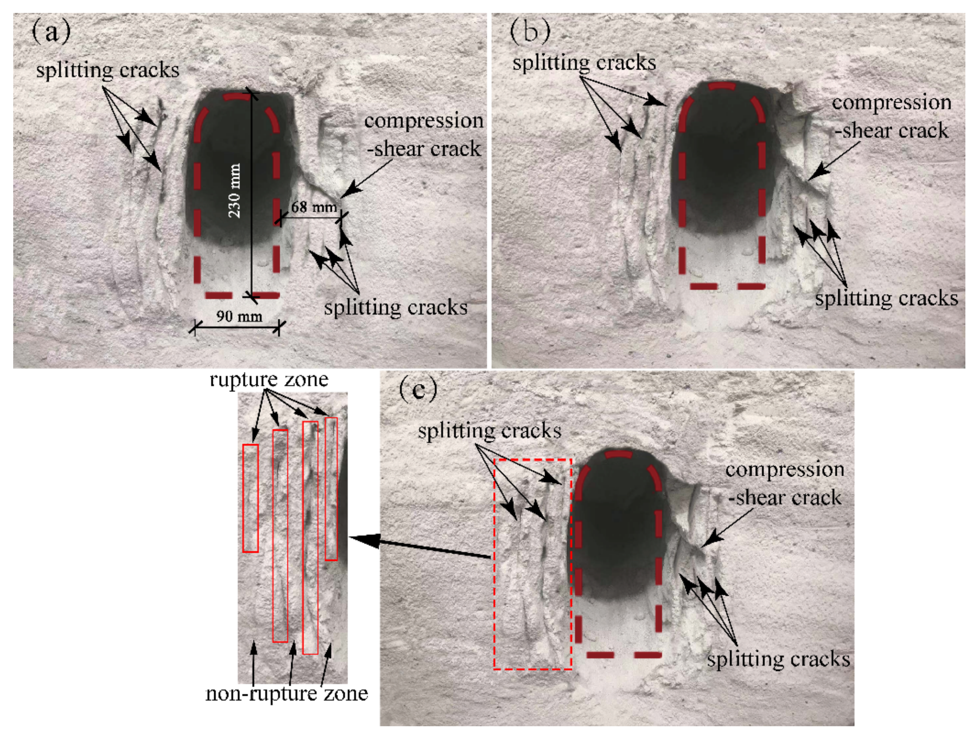
Figure 9.
The fracture mode of the splitting failure model test of the high sidewall cavern. (a) 100 mm from the front boundary of the model; (b) 200 mm from the front boundary of the model; (c) 300 mm from the front boundary of the model [50].
Figure 9.
The fracture mode of the splitting failure model test of the high sidewall cavern. (a) 100 mm from the front boundary of the model; (b) 200 mm from the front boundary of the model; (c) 300 mm from the front boundary of the model [50].

Figure 10.
Variation of the radial displacement around the cavern.

Figure 11.
Variation of the radial stress around the cavern.

Figure 12.
Variation of the tangential stress around the cavern.

Figure 13.
Variation of tangential stress of high side wall caverns with different height–span ratios.
Figure 13.
Variation of tangential stress of high side wall caverns with different height–span ratios.


Table 1.
The parameters of the mapping function.
| c | a1 | a2 | a3 | a4 |
|---|---|---|---|---|
| 1.512308 | 0.269926 | 0.029007 | 0.366010 | −0.158103 |
Table 2.
Rock parameters in theoretical calculation.
| Initial Elastic Modulus/GPa | Unit Weight/(KN·m−3) | Compressive Strength/MPa | Tensile Strength/MPa | Peak Strain | Ultimate Strain | Poisson’s Ratio | Lame Constant/GPa | Internal Length Parameter/m |
|---|---|---|---|---|---|---|---|---|
| 41.50 | 26.60 | 128.80 | 8.00 | 0.27 | 16.34 | 0.01 |
Table 3.
Radial displacement around the cavern.
| Location | Category | Radial Displacement Value/mm | |||||
|---|---|---|---|---|---|---|---|
| 0.1 L | 0.5 L | L | 1.5 L | 2 L | 3 L | ||
| Right sidewall | Model test | 63.0 | 27.0 | 36.0 | 9.0 | 18.0 | 3.0 |
| Theoretical calculation | 58.30 | 14.34 | 30.82 | 4.82 | 10.94 | 0.30 | |
| Right hance | Model test | 57.0 | 24.0 | 30.0 | 7.5 | 15.0 | 3.0 |
| Theoretical calculation | 49.92 | 12.98 | 25.48 | 3.50 | 9.71 | 0.30 | |
| Vault | Model test | 42.0 | 30.0 | 24.0 | 15.0 | 9.0 | |
| Theoretical calculation | 32.75 | 12.81 | 10.17 | 3.24 | 0.14 | ||
| Left hance | Model test | 57.0 | 18.0 | 33.0 | 7.5 | 15.0 | 1.5 |
| Theoretical calculation | 49.92 | 12.98 | 25.48 | 3.50 | 9.71 | 0.30 | |
| Left sidewall | Model test | 64.5 | 21.0 | 34.5 | 6.0 | 16.5 | 1.5 |
| Theoretical calculation | 58.30 | 14.34 | 30.82 | 4.82 | 10.94 | 0.30 | |
Table 4.
Radial stress around the cavern.
| Location | Category | Radial Stress Value/MPa | |||||
|---|---|---|---|---|---|---|---|
| 0.1 L | 0.5 L | L | 1.5 L | 2 L | 3 L | ||
| Right sidewall | Model test | −1.32 | −6.20 | −4.90 | −8.61 | −7.96 | −11.77 |
| Theoretical calculation | −2.62 | −8.33 | −4.90 | −9.68 | −9.13 | −12.76 | |
| Right hance | Model test | −1.22 | −7.24 | −4.79 | −9.59 | −8.89 | −12.57 |
| Theoretical calculation | −3.82 | −8.53 | −7.07 | −10.67 | −10.31 | −13.45 | |
| Vault | Model test | −2.08 | −6.94 | −8.21 | −10.39 | −12.63 | |
| Theoretical calculation | −4.50 | −8.36 | −10.41 | −12.41 | −14.08 | ||
| Left hance | Model test | −1.38 | −7.57 | −4.90 | −9.12 | −8.21 | −11.93 |
| Theoretical calculation | −3.82 | −8.53 | −7.07 | −10.67 | −10.31 | −13.45 | |
| Left sidewall | Model test | −1.82 | −6.60 | −4.88 | −8.17 | −7.98 | −11.85 |
| Theoretical calculation | −2.62 | −8.33 | −4.90 | −9.68 | −9.13 | −12.76 | |
Table 5.
Tangential stress around the cavern.
| Location | Category | Tangential Stress Value/MPa | |||||
|---|---|---|---|---|---|---|---|
| 0.1 L | 0.5 L | L | 1.5 L | 2 L | 3 L | ||
| Right sidewall | Model test | −3.83 | −6.94 | −20.36 | −17.48 | −19.38 | −16.08 |
| Theoretical calculation | −4.82 | −12.13 | −26.29 | −22.34 | −23.51 | −17.28 | |
| Right hance | Model test | −2.09 | −8.39 | −19.91 | −16.99 | −18.68 | −16.39 |
| Theoretical calculation | −5.33 | −12.77 | −24.16 | −21.16 | −22.75 | −16.79 | |
| Vault | Model test | −23.39 | −19.83 | −16.4 | −15.88 | −15.12 | |
| Theoretical calculation | −26.59 | −23.49 | −20.46 | −19.55 | −17.62 | ||
| Left hance | Model test | −2.92 | −9.24 | −19.35 | −17.72 | −19.55 | −16.18 |
| Theoretical calculation | −5.33 | −12.77 | −24.16 | −21.16 | −22.75 | −16.79 | |
| Left sidewall | Model test | −2.07 | −8.58 | −18.71 | −17.95 | −19.29 | −16.97 |
| Theoretical calculation | −4.82 | −12.13 | −26.29 | −22.34 | −23.51 | −17.28 | |
Publisher’s Note: MDPI stays neutral with regard to jurisdictional claims in published maps and institutional affiliations. |
© 2021 by the authors. Licensee MDPI, Basel, Switzerland. This article is an open access article distributed under the terms and conditions of the Creative Commons Attribution (CC BY) license (https://creativecommons.org/licenses/by/4.0/).
Share and Cite
MDPI and ACS Style
Li, F.; Zhang, Q.; Xiang, W. Mechanism of Splitting Failure for High Sidewall Cavern of Hydropower Station Based on Complex Function and Strain Gradient. Energies 2021, 14, 5870. https://0-doi-org.brum.beds.ac.uk/10.3390/en14185870
AMA Style
Li F, Zhang Q, Xiang W. Mechanism of Splitting Failure for High Sidewall Cavern of Hydropower Station Based on Complex Function and Strain Gradient. Energies. 2021; 14(18):5870. https://0-doi-org.brum.beds.ac.uk/10.3390/en14185870
Chicago/Turabian StyleLi, Fan, Qiangyong Zhang, and Wen Xiang. 2021. "Mechanism of Splitting Failure for High Sidewall Cavern of Hydropower Station Based on Complex Function and Strain Gradient" Energies 14, no. 18: 5870. https://0-doi-org.brum.beds.ac.uk/10.3390/en14185870
Note that from the first issue of 2016, this journal uses article numbers instead of page numbers. See further details here.