
A Two-Stage Short-Term Load Forecasting Method Using Long Short-Term Memory and Multilayer Perceptron

1
Research Center for Advanced Science and Technology, School of Engineering, The University of Tokyo, 4-6-1 Komaba Meguro-ku, Tokyo 1538904, Japan
2
School of Engineering, Tokyo University of Science, 6-3-1 Niijuku Katsushika-ku, Tokyo 1258585, Japan
*
Author to whom correspondence should be addressed.
Energies 2021, 14(18), 5873; https://0-doi-org.brum.beds.ac.uk/10.3390/en14185873
Submission received: 18 August 2021
/
Revised: 5 September 2021
/
Accepted: 7 September 2021
/
Published: 16 September 2021
(This article belongs to the Section F: Electrical Engineering)
Abstract
:Load forecasting is an essential task in the operation management of a power system. Electric power companies utilize short-term load forecasting (STLF) technology to make reasonable power generation plans. A forecasting model with low prediction errors helps reduce operating costs and risks for the operators. In recent years, machine learning has become one of the most popular technologies for load forecasting. In this paper, a two-stage STLF model based on long short-term memory (LSTM) and multilayer perceptron (MLP), which improves the forecasting accuracy over the entire time horizon, is proposed. In the first stage, a sequence-to-sequence (seq2seq) architecture, which can handle a multi-sequence of input to extract more features of historical data than that of single sequence, is used to make multistep predictions. In the second stage, the MLP is used for residual modification by perceiving other information that the LSTM cannot. To construct the model, we collected the electrical load, calendar, and meteorological records of Kanto region in Japan for four years. Unlike other LSTM-based hybrid architectures, the proposed model uses two independent neural networks instead of making the neural network deeper by concatenating a series of LSTM cells and convolutional neural networks (CNNs). Therefore, the proposed model is easy to be trained and more interpretable. The seq2seq module performs well in the first few hours of the predictions. The MLP inherits the advantage of the seq2seq module and improves the results by feeding artificially selected features both from historical data and information of the target day. Compared to the LSTM-AM model and single MLP model, the mean absolute percentage error (MAPE) of the proposed model decreases from 2.82% and 2.65% to 2%, respectively. The results demonstrate that the MLP helps improve the prediction accuracy of seq2seq module and the proposed model achieves better performance than other popular models. In addition, this paper also reveals the reason why the MLP achieves the improvement.
1. Introduction
Electricity is an essential guarantee for industrial production and social life. To meet the consumers’ satisfaction and generate profit, electric power companies should balance the supply and need by scheduling a series of generators in the most efficient manner. In the long term, the investment in power grids and power plants also needs to keep pace with the increasing power demand. Both in short-term generation dispatch and long-term planning, load forecasting is indispensable for decision-making. Studies have shown that only a 1% decrease in the mean absolute percentage error (MAPE) of load forecasting has a consequential impact of 3∼5% on the supply side by reducing the cost of generation by about 0.1∼0.3% [1]. For instance, a 1% increase in load forecasting error resulted in incremental operating costs of up to 10 million pounds per year in the thermal British power system, reported in 1986 [2]. Load forecasting can be categorized into four types [3] according to different predicted periods: very short-term load forecasting (VSTLF), short-term load forecasting (STLF), medium-term load forecasting (MTLF), and long-term load forecasting (LTLF), shown in Table 1.
In this paper, we focus on the STLF, which is essential to generation dispatch. The operators of power system need to make power generation plans in advance to achieve economical and reliable operation. With the economic growth, the electricity demand continues to increase. The emergence of a large number of electric vehicles and various household appliances has brought more uncertainties to the management of power grids. In addition, the increase in intermittent renewable energy sources (RES) connected to the electricity networks, especially photovoltaic and wind turbine, makes the management of power systems more challenging. The increased RES penetration has raised the need for spinning reserves to offset the fluctuation of RES generation [4]. These two new challenges have forced electric power companies to improve their operational capabilities. Therefore, decision-makers have higher requirements for the accuracy of load forecasting.
A wide variety of methods for STLF have been reported in the literature. The conventional techniques for STLF include knowledge-based approaches and statistical models. The expert system [5] is a classical approach that uses expert knowledge and experience to predict the load demand. However, the expert system has some drawbacks, such as difficulty in creating inference rules, inability to learn by itself, and heavy manual updates. Relatively speaking, statistical methods are more popular, including general exponential smoothing (GES) [6], multiple linear regression (MLR) [7], and autoregressive integrated moving average (ARIMA) [8,9]. Although these methods can build understandable models, the prediction accuracy for STLF is poor due to the inherent non-linearity of electricity consumption.
In recent years, computational intelligence (CI) methods are widely used in research works. The CI is a set of nature-inspired computational algorithms to address complex real-world problems to which mathematical or traditional modeling can be useless [10]. The unique strength of CI methods is their powerful ability of autonomous mapping between the input and output without complicated mathematical formulation, namely black box. Furthermore, the CI methods are expert in dealing with non-linear problems. The most commonly used CI methods in STLF are fuzzy logic [11,12], support vector machine (SVM) [13,14], and artificial neural networks (ANN) [15,16,17,18,19,20,21,22,23]. Researchers used shallow neural networks, such as multilayer perceptron (MLP) and simple recurrent neural network (RNN), to construct the load forecasting model in early literature. In [16], Hayati M. et al. proposed a MLP model to forecast the next 24 h load of Illam region in Nepal. The model directly uses the previous 24 h load and meteorological data as the inputs without feature selection. Thus, the performance of the model is poor, which gives the MAPE of 18%. In [17], Ding N. et al. presented the model selection and feature selection methods to optimize the MLP model. The results show that the design methodology helps to obtain the optimal model given the available data. However, authors did not take the impacts of holidays and seasons on power consumption into account. Lee K.Y. et al. [18] reported that the RNN model performs better than the MLP model because it uses fewer neurons and weights, trains faster, and gives higher accuracy. In 1992, Lee K.Y. et al. [19] presented a diagonal recurrent neural network (FRNN) to improve training efficiency and prediction accuracy. The RNN uses its internal memory cell to process sequences of inputs. However, when the sequences become very long, gradient vanishing and exploding problems often lead to failure in training. A variant of RNN, long short-term memory (LSTM), was initially introduced by Hochreiter et al. [24] to tackle these problems. Applications of the LSTM networks have been reported in different areas, especially in natural language processing [20]. To develop the LSTM’s potential, it is generally used in deep neural networks to solve practical problems. Marino D.L. et al. [21] investigated two deep neural networks (DNN) using the LSTM to forecast the next 60 h load demand for an individual building. The results showed that the LSTM-based sequence to sequence (seq2seq) architecture outperforms the standard LSTM network. Both models solely take the historical load as the inputs without considering temperature, holidays, and seasons. The accuracy of predictions over peaks and valleys is poor. In [22], the presented LSTM framework for the STLF of residential households. The results demonstrated that the proposed model is superior to other algorithms and performs better in aggregating load forecast than individual load forecast. Similarly to the former work, none of the temperature, holidays, and seasons are considered. The MAPE of aggregating load forecast reaches up to 8%. Another type of ANN, the convolutional neural networks (CNN), which is good at feature extraction and widely used for image recognition, was adopted to make load forecasts. Kuo P.H. et al. [23] presented a one-dimensional (1D) CNN with three convolution layers for STLF. The results show that the CNN model outperforms other single machine learning methods under the given dataset. The power consumption is highly related to the type of day, season, and temperature. Meanwhile, the power consumption is an inertial and non-linear system. The load itself is strongly correlated to the load of the previous hours. The MLP is good at modeling non-linear tasks. However, it is highly dependent on proper feature selection. Nevertheless, artificial feature selection will inevitably lead to information loss, especially temporal features. The LSTM and CNN models can extract temporal features from the inputs. However, limited to the network topologies in previous literature, none of those models considers all essential features.
To take advantage of different methods, researchers try to find out proper combinations of them to make more precise predictions. A hybrid STLF model using ARIMA and SVM is proposed by Nie H. et al. [25]. It firstly uses ARIMA to obtain the preliminary 24-h forecasts and then uses SVM to correct the deviation of the previous predictions. The results show that the MAPE decreases from 4.5% to 3.85%. Because the ARIMA model can only handle one-sequence to one-sequence tasks, it takes the load itself as the input without considering other features. In addition, the feature selection for the SVM is not reported. In [26], Tian C. et al. presented a DNN model for STLF based on SLTM and CNN. The CNN and LSTM are used to extract the local trend and temporal features of the load, respectively. None of the temperature, holiday, and season is considered. The results show that the CNN-LSTM model gives the lowest average MAPE but fails to show the improvement over peaks and valleys. David K. et al. [27] presented a convolutional LSTM for short-term temperature forecasts. The results reveal that the univariate LSTM network performs well in the first few hours but is outperformed by the multivariate LSTM network. Moon J. et al. [28] proposed a hybrid STLF model for different buildings in a university campus combining random forest (RF) and the MLP. The RF is used to group different buildings into an academic cluster, engineering cluster, and dormitory cluster. The results demonstrate that the proposed model is superior to other popular models. However, this method is inapplicable for regional load forecast. In 2017, Google teams shouted, “Attention is all you need”. Ref. [29] making the attention mechanism (AM) more famous in deep learning (DL). Wang S.X. et al. [30] presented a bi-directional LSTM model with the AM. The results show that the MAPE decreases from 3.43% to 2.77% by adding an attention layer to the traditional Bi-LSTM model.
We found that the LSTM-based hybrid model predominates in STLF. The LSTM-base model performs very well over the first few hours of the predictions but is unsatisfactory for the next few hours. How to obtain preliminary predictions with high accuracy using LSTM-based model and improve the predictions over the entire time horizon is an open issue. Based on the outcomes of the previous works, we presents a two-stage STLF method using the LSTM, AM, and MLP. An LSTM-based seq2seq forecasting module with the AM is constructed to make 24-h predictions in the first stage, which can process a multi-sequence of input. When training the seq2seq module, the LSTM can only learn from the known information before the target day. However, the knowledge of the target day also plays an important role in the predictions. Therefore, in the second stage, the preliminary results obtained in the first stage are fed into the MLP network to make point to point (p2p) predictions along with the information about temperature and holiday of the target day and the missing features that the seq2seq module cannot capture. We evaluate the performance of the seq2seq module under different lengths of the input window, namely timestep. For example, when using the previous seven days’ data to predict the next 24 h load, the timestep is 168 h. We collected the power cunsumption and weather records of Kanto region from 2016 to 2019 to train the proposed model. The contributions of this study are as follows:
- A two-stage method for STLF that consists of an LSTM-based seq2seq module and an MLP-based p2p module, which outperforms other popular models, is proposed. The seq2seq module is capable to handle a multi-sequence of input, so that the model can capture more features. In the second stage, given proper input features, the forecasting errors of the predictions obtained by the seq2seq module are reduced;
- The impact of the timestep for the seq2seq module is investigated. The experimental result shows that a timestep of 24 h is the best choice in this case. The hyperparameters tunning results are presented for reference;
- This study reveals that feeding multi-sequence of input to the LSTM makes it adapt to variations of seasons, holidays, and temperature. Therefore, the model does not need to be frequently updated. Although the MLP module inherits the advantage of the seq2seq module and improves the residual distribution by learning the variation tendency of load affected by holidays, seasons, and temperature;
- Research directions regarding the improvement and generalization in time series forecasting problems, using the MLP as a residual modifier, are highlighted.
The rest of this paper is organized as follows. Section 2 introduces the methodologies employed in this paper. In Section 3, we describe the proposed model and evaluation indices. Section 4 presents the dataset, data preprocessing, and experimental results. In Section 5, we discuss the results and point out future research directions.
2. Applied Methodologies
To better understand the framework of the proposed STLF model, this section introduces the relevant methods, including RNN, LSTM, AM, and MLP.
2.1. Recurrent Neural Network
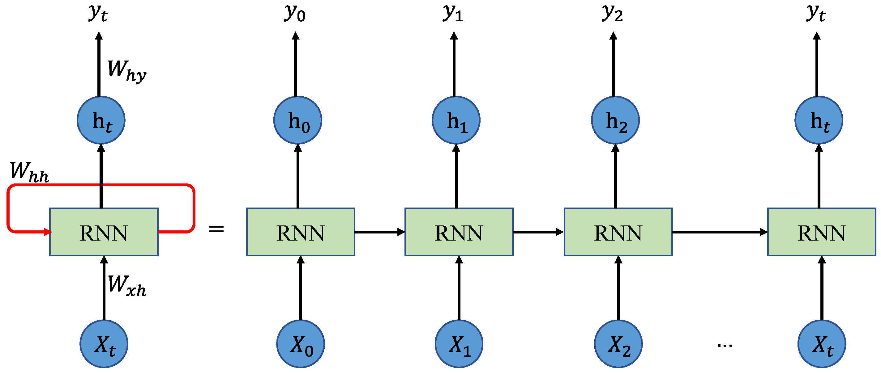
The RNN is a generalization of feedforward neural network that has an internal state (i.e., memory), making it applicable to process sequences of inputs, such as speech recognition [31], natural language processing [32], and time series prediction [18,19]. When processing a sequence of input, the RNN performs the same function for each input of data. After producing the output of current input of data, it is duplicated and sent back into the RNN as a component of the next input. Figure 1 shows the structure of a simple RNN. The mapping from the input to output can be described using following equations [31]:
where is the hidden state at time t; , , and are shared weight matrix at current input state, previous hidden state, and output state, respectively; and are the activation functions.
Initially, the RNN takes from the sequence of input and generates hidden state and output . In the next step, and are the input. The RNN repeats this process till the end of the sequence. In this way, the RNN keeps remembering the previous information. Thus, it is good at processing the sequence whose contexts are intrinsically related. However, the RNN is trained using backpropagation algorithm, and, therefore, gradient vanishing problem may occur when the sequence became very long.
2.2. Long Short-Term Memory
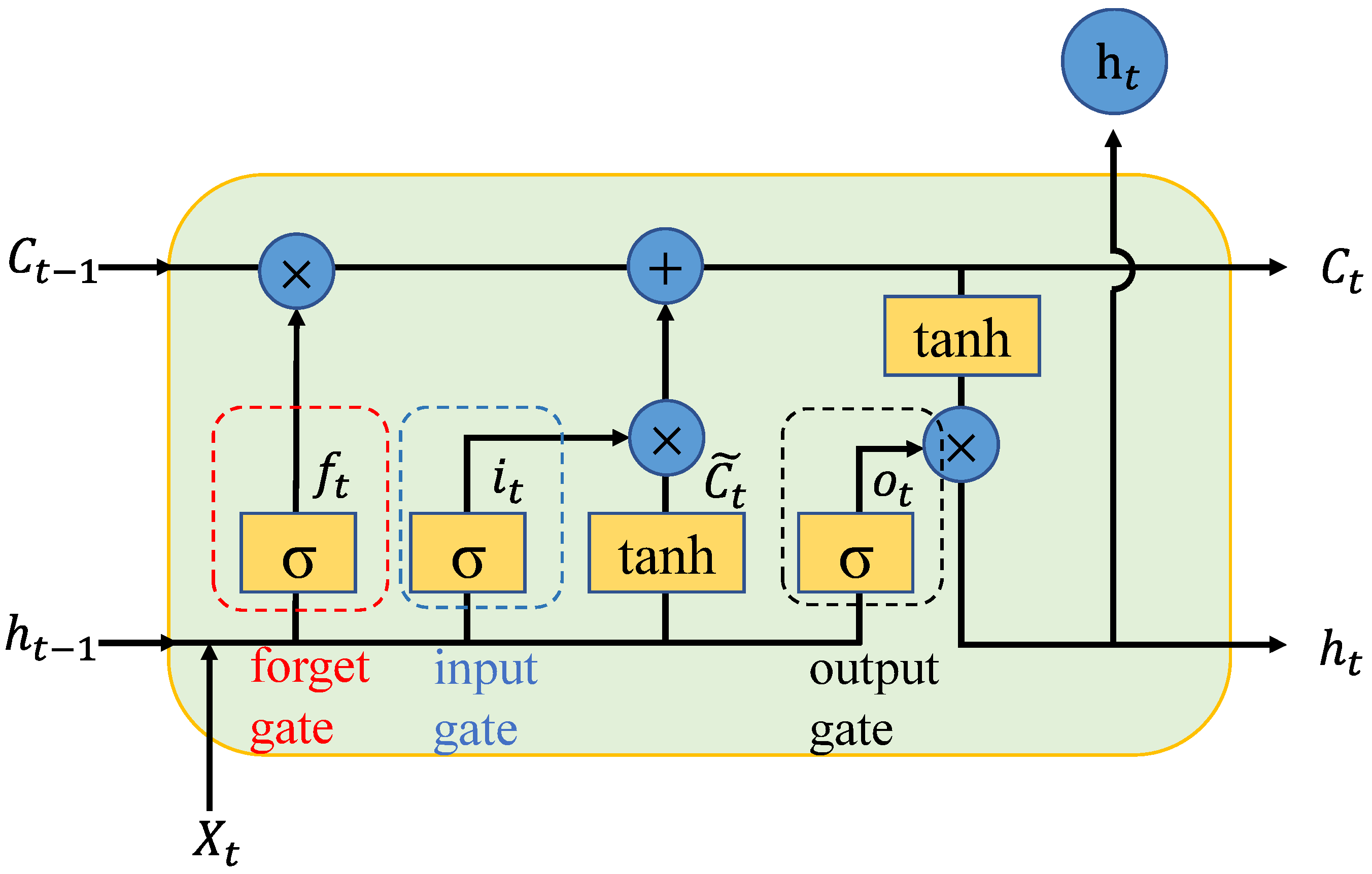
The LSTM network is a variant of RNN, which has several gates to control the input, memory (i.e., cell state), and output, making it remembers past information more efficiently [26]. So that the gradient vanishing problem is resolved. The structure of an LSTM network is shown in Figure 2.
When the LSTM processing a sequence, the first step is to decide what information in the memory will be thrown. The decision is made by the forget gate via the Sigmoid function, whose output is a value between 0 and 1. The larger the output value is, the more past information is kept in the memory. The calculation of the forget gate can be expressed as [27]:
where and are the weight matrix and bias of the forget layer, is the output (i.e., hidden state) at time , is the input of current state.
The next step is to determine what new information will be stored in the memory by the input gate. The tanh layer creates a candidate of the input. Meanwhile, the input gate will generate a value between 0 and 1 through the Sigmoid layer. The candidate, , will be scaled by and added to the memory to update the cell state . The calculations of , , and are as follows [27]:
where and are the weight matrix and bias of the tanh layer, and are the weight and bias of the Sigmoid layer of the input gate, respectively.
Finally, the LSTM gives the output controlled by the output gate. We put the current cell state through a tanh layer and multiply it by the scalar generated by the output gate. The scalar and output of the LSTM can be computed by [27]
where and are the weight and bias of the Sigmoid layer of the output gate, respectively.
2.3. Attention Mechanism
The AM in DL is based on the concept of directing the focus, making the networks pay greater attention to certain factors when processing the input of data. In this study, we employed a self-attention layer to enhance the performance of the seq2seq model [33]. It is used to manage and quantify the interdependence within the elements of the input sequence. Therefore, when generating the output over any timestep, this layer has viewed the whole input sequence and captured the relationships between any two timeslots.
An self-attention mechanism can be described as mapping a query and a set of key-value pairs to an output. The self-attention layer operates an input sequence, where , and generates a new sequence where . The query, keys, and values are computed by [33]
where , , are the training parameters.
The output is computed as weighted sum of a linear transformed input elements [33]:
The represents the weight coefficient between elements and , which is computed using a softmax function [33]:
The attention score can be calculated by [33]
2.4. Multilayer Perceptron
The MLP is a class of feedforward ANNs, consisting of a series of interconnected neurons (i.e., nodes). The structure of a simple MLP network [34] with one hidden layer is shown in Figure 3. The network consists of an input layer with d units, one hidden layer with m units, and one output layer with one node. Since MLP networks are fully connected, each node in one layer connects with a certain weight to every node in the following layer. The outcomes of the MLP can be described by Equation (15) [34].
where denotes the weight from neuron of input layer to neuron of hidden layer, denotes the weight from neuron of hidden layer to output layer, and is the activation function. One commonly used activation function is the rectified linear unit (ReLU) function, which can be written as:
The MLP can approximate highly non-linear functions between the input and output without any complex mathematical formula. It has been approved that the performance of MLP in forecasting applications outperforms regression-based methods [35]. Depending on different cases, the MLP may have more than one hidden layer and multiple units in the output layer.
3. The Proposed Model
This section presents the framework of the two-stage forecasting model. A seq2seq forecasting module is used to forecast the next 24 h load demand in the first stage. In the second stage, the MLP module makes p2p predictions based on the outcomes of the seq2seq module, which functioned as a residual modifier. Each element of the output sequence obtained in the first stage will be fed into the MLP along with holiday and temperature information, as well as lagged load demand, giving the final predictions. To evaluate the forecasting accuracy, several criteria are introduced.
3.1. The Framework of the Proposed Model
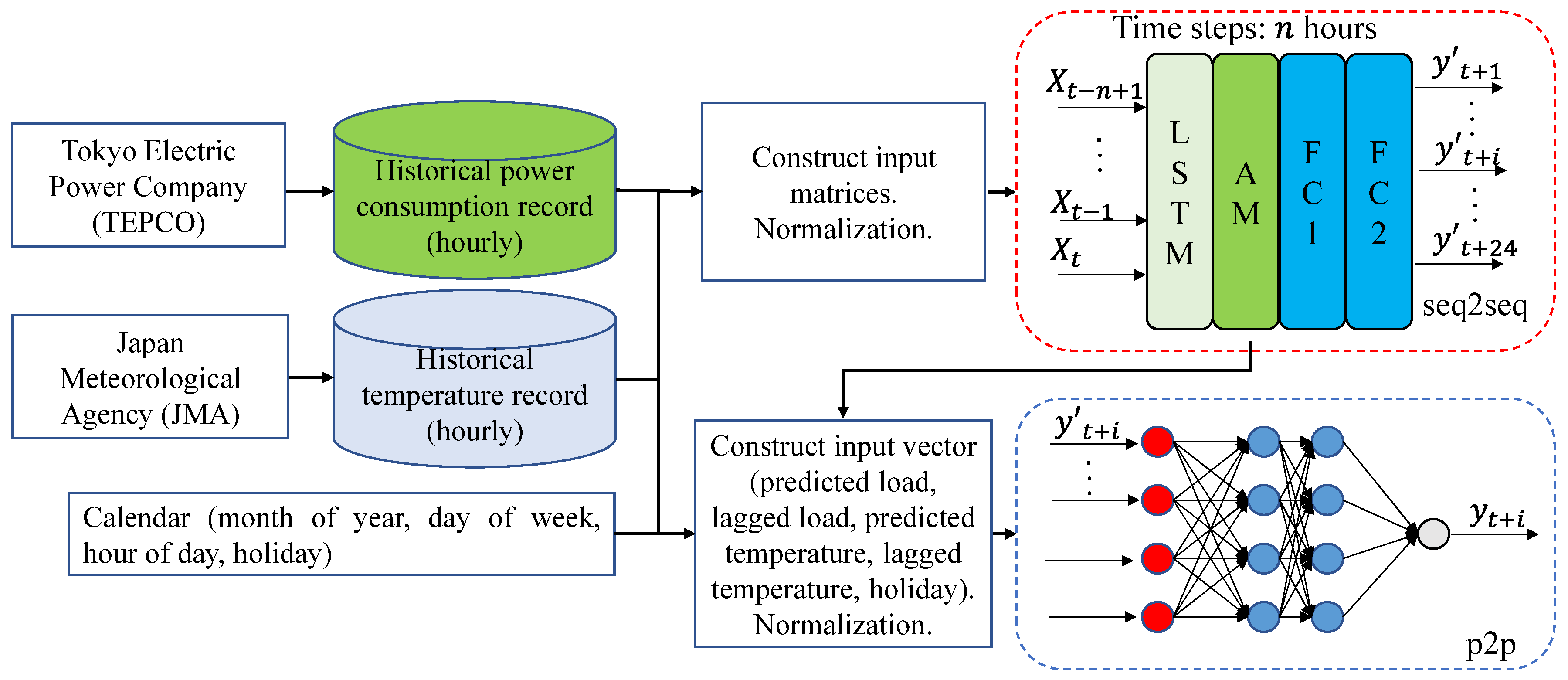
The framework of the two-stage forecasting model is shown in Figure 4. The proposed model consists of an LSTM-based module with the AM for multi-step forecasting and an MLP-based module for residual modification. The inputs of the seq2seq module are over the past n hours where n is the length of the input window, including (month of year, 1 to 12 represent January to December), (day of week, 1 to 7 represent Monday to Sunday), (hour of day, 0 to 23 represent 0:00∼1:00 to 23:00∼24:00), (load), and (temperature). At time t, the seq2seq module processes the input, , where and outputs the predictions of the next 24 h load demand via the fully connected (FC) layer, .
We selected ten features as the input of the MLP network, including , , (holiday, 1 represents holiday, 0 represents workday), (holiday to workday, 1 represents that the previous day is a holiday and the target day is a workday, otherwise is 0), (168-h lagged load), (mean load of the same hour of previous three days), (predicted load in the first stage), (168-h lagged temperature), (24-h lagged temperature), (predicted temperature by a trained ARIMA model [9]). The input vector, , , is fed into the MLP module to modify the residue of the predicted load , giving the final prediction.
3.2. Evaluation Indices
Several criteria are used as the evaluation indices to justify the performance of load forecasting models, also called key performance indicator (KPI). In this paper, we choose the mean absolute percentage error (MAPE) and root mean squared error (RMSE) as the indicators. The calculations of these two indices [25] are as follows:
where k is the size of the samples, and represent the predicted value and observed value, respectively. The MAPE shows the mean of the dispersion between predictions and ground truth. On the other hand, the RMSE describes the standard deviation of the differences between the predicted values and observed values. The smaller values of the above KPIs, the better performance of the model is.
4. Experiments
The experiments are carried out under the environment of Python 3.6 with the Keras (2.2.4) [36] of Tensorflow 2.1.0, using a computer with following specification: window 10, 1.80 GHz 64-Bit Intel Core i7-8565U processor.
The proposed model is trained and examined using the load record and temperature record of Tokyo. In this section, experiments regarding the selection of timestep are presented. The performance of the proposed model is compared with the conventional models.
4.1. Dataset Description
The dataset used in the paper consists of load records, temperature records, and calendar. The load records of Tokyo are collected from the website of Tokyo Electric Power Company (TEPCO), and the temperature records are obtained from the website of Japan Meteorological Agency (JMA). The service areas of TEPCO includes Tokyo and other adjacent cities. We use the mean temperature of three major cities (Tokyo, Kanagawa, Gunma) for training. The interval of the load records and temperature records is one hour. The information about holiday is extracted from the calendar of Japan. The period of the dataset is from 1 April 2016 to 31 December 2019. The dataset, which contains 32,880 samples, is split into a training set (80%) and a validation set (20%). We test the losses of the seq2seq model under different splitting ratios. The results are listed in Table 2. We choose the splitting ratio with lower validation loss. Figure 5 shows the hourly load profile.
4.2. Data Preprocessing
4.2.1. Data Cleaning
Both the load dataset and temperature dataset have no outlier, which is examined by Tukey‘s test (i.e., box-plot). In the temperature dataset, there are 30 discrete missing points in total. The missing values are filled using the value of the previous hour, considering the inertia of temperature.
4.2.2. Temperature Adjustment
In the MLR and MLP model, the temperature is adjusted by Equation (19) considering the load is non-linear to the temperature.
where is the temperature at time i, is the baseline which is set to 18 C. The load demand increases for cooling while the temperature is getting higher comparing to the baseline. Likewise, the load demand increases for heating along with the decrease in the temperature. The Person correlation between load and temperature increases from 0.09 to 0.56 after the adjustment.
4.2.3. Feature Scaling
Feature scaling is an essential step for training neural networks. In this paper, standardization is applied, which transforms the data to have zero mean and a variance of one using the following equation:
where and are the mean value and standard deviation of feature X, respectively.
4.3. Experimental Results
4.3.1. Experimental Setting
In the seq2seq module, we used an LSTM layer with 100 units. The hidden fully connected layer (FC1) has 64 nodes with an activation function of the ReLU. The loss is defined as the MAE. The epochs and batch size are 50 and 32, respectively. To select a proper length of input window, we performed a series of experiments by setting the length of input window .
In the p2p module, the number of nodes of the input layer and output layer are ten and one, respectively. The numbers of hidden layers and nodes of each hidden layer are two and 100, respectively. The activation function of hidden layers is the ReLU. The loss is defined as the MAE. The number of epochs is 100.
The arguments employed in the seq2seq module and p2p module are determined through a series of hyperparameter tuning tests. We evaluate the validation losses of the models under different hyperparameters. Table 3 and Table 4 show the results of the hyperparameter tuning for the seq2seq module. The results for the p2p module are listed in Table 5 and Table 6. We choose the settings whose validation loss is the lowest.
4.3.2. Selection of TimeStep
We experimented with the seq2seq model by changing the timestep from 24 to 168. For instance, when , it means that we use the previous seven days’ data to predict the load of the next day. The results are listed in Table 7.
According to the results, we set the timestep as 24 h to construct the seq2seq module. From the previous literature, we knew that the future load has strong correlations with the load over the same hour of the last three days and seven days. However, the seq2seq module with a timestep of 24 h resulted in missing the information mentioned earlier. Therefore, in the second stage, we consider involving the missing data in the MLP module.
4.3.3. Results and Comparison
In order to demonstrate the superiority of the proposed STLF model, the traditional MLR model, MLP model, CNN model, standard LSTM model with one sequence of input, standard LSTM model without AM, and LSTM model with AM are selected for comparison in terms of the MAPE and RMSE. Any LSTM model other than the LSTM(1seq), as hereinafter defined, has a default multi-sequence of input. Both the MLR model and MLP model select ten features, which is similar to the MLP module introduced in Section 3.1. The difference is that the (predicted load) is replaced by (24-h lagged load). In the CNN model, the kernel size of the Conv1D layer and the pool size of the MaxPooling1D are both 3. The settings of LSTM-based and MLP-based models are exactly the same as the settings presented in Section 4.3.1.
As shown in Table 8, the evaluation indices of the proposed model are the smallest among the six models. The results reveal that ANN-based models outperform the regression-based model. The MLP model gives a MAPE of 2.65% which lower than other single ANN networks. The results also show that the AM helps increase the forecasting accuracy of the LSTM-based model. By modifying the seq2seq module’s residual, the proposed model gives a MAPE and RMSE of 2% and 1, respectively. Compared to the LSTM-AM model and MLP model, the performance of the proposed model improves by 29.1% and 24.5% in terms of the MAPE, respectively.
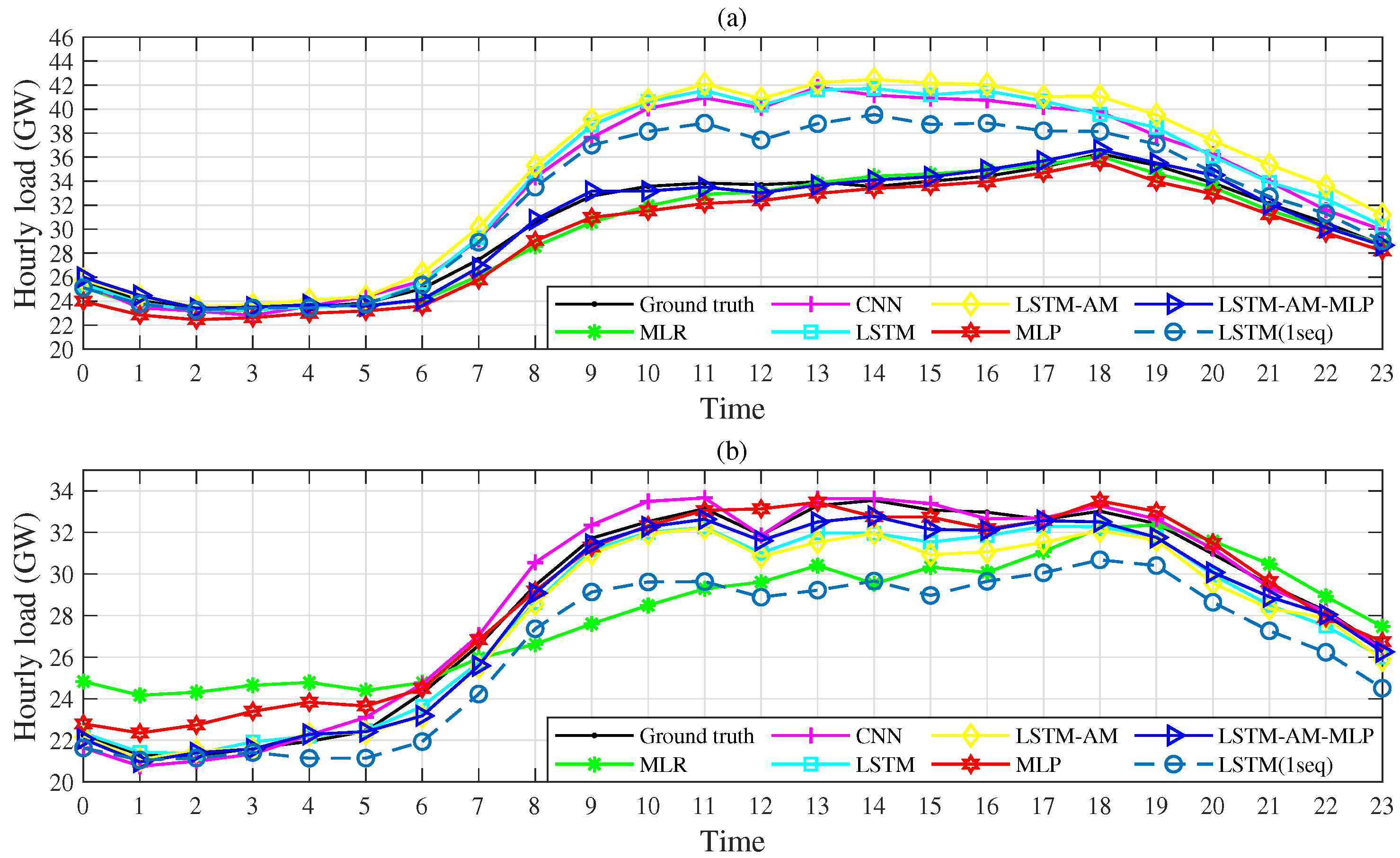
Figure 6 shows the forecasting results of six models on a specific holiday and a workday. As we can see, the results given by the LSTM-AM model perform very well during the morning time. That is because of the user’s behavior of inertial and less uncertainty. On the other hand, LSTM-based models are proficient in the analysis of time series. However, the forecasting errors become larger after 8:00 a.m. The predictions after 8:00 a.m. on the same day are either all underestimated or all overestimated. Fortunately, the trend is in line with the ground truth. Therefore, it is possible to calibrate the forecasting errors (i.e., residuals) following certain rules.
Compared to the LSTM-AM model, predictions of the proposed model change little before 8:00 am and are pulled towards the ground truth after 8:00 am. Both on the holiday and workday, the proposed model is superior to other models. We guess the MLP module helps improve the prediction accuracy because in the second stage of the proposed model it inherits the precise predictions of the seq2seq module in the morning time and modifies the residuals. To verify our hypothesis, we analyze the residuals of the LSTM-AM model and LSTM-AM-MLP model. The definition of the residual can be expressed by
where is the predicted value and is the observed value. Thus, a positive residual represents overestimation, and a negative residual represents an underestimate.
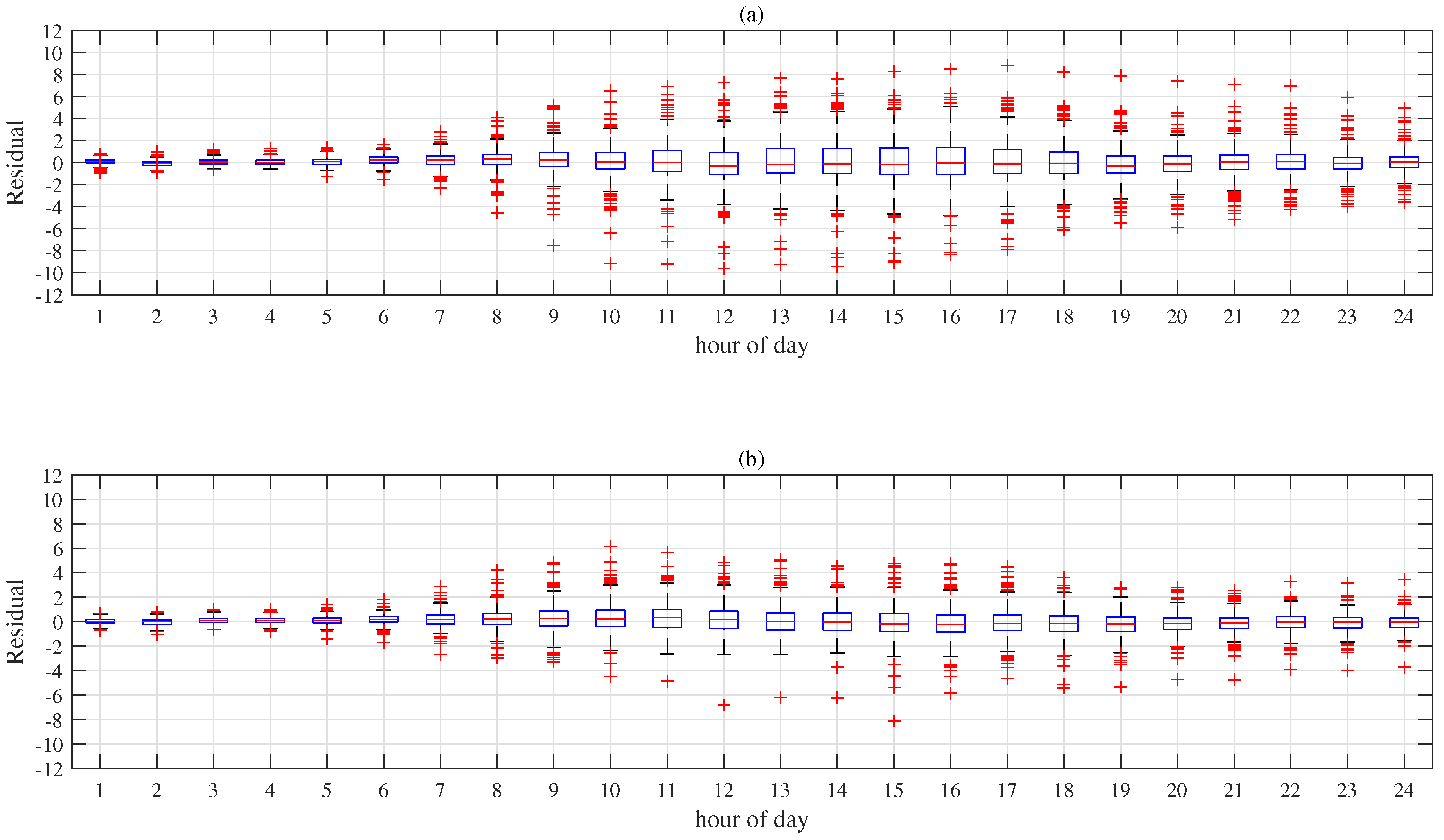
As we can see in Figure 7, the residuals of the LSTM-AM model in the morning time are relatively low and stable. The conclusion is consistent with the forecasting results on the specific holiday and workday. In the following hours of day, the residuals are gradually getting divergent. For the LSTM-AM-MLP model, the residual’s distributions in the morning time are very close to those of the LSTM-AM model. In the following hours of day, the heights of boxes are significantly shorter. In other words, the predictions during those hours are convergent to the ground truth. In order to show overall distribution of the residuals, we plot the histograms for both LSTM-AM model and LSTM-AM-MLP model, shown in Figure 8. The proposed model gives 78.9% of the predictions with a residual within −1 and 1, which is 9.4% higher than that of the LSTM-AM model. The results explain our assumption about the reason why the MLP module helps improve the performance.
5. Discussion
To determine the length of the input window, a series of experiments are carried out. Usually, when increasing the input of the neural network, the model is expected to have a better performance. However, in this case, the error is growing along with the increase in timestep. The result provides a reference for choosing an appropriate timestep, but it cannot explain the abnormal fact. It remains an open issue for future works.
This study compared six independent models for STLF, including the MLR, MLP, CNN, LSTM(1seq) without AM, LSTM without AM, and LSTM with AM. The MLR is a simple regression model. It is easy to understand the mapping from the input to the output. However, the MLR cannot deal with non-linear tasks so that the performance is far from the MLP in spite of given the same inputs. The MLP is outstanding among the six models because of the proper feature selection. However, the performance over the first few hours of the target day is not as good as the LSTM model both on the holiday and workday. The results also show that the LSTM(1seq) model performs poorly, while the LSTM model is greatly improved. In other words, feeding information about month of year, day of week, hour of day, and temperature to the LSTM helps reduce the forecasting error. The CNN model performs much better on workdays than on holidays. On the other hand, the LSTM model has a more balanced performance on both types of days. The MAPE of LSTM model is lower than that of CNN model. The LSTM model with AM is better than the model without AM. To sum up, the proposed LSTM-AM model with a multi-sequence of input outperforms other single models except for the MLP model, offering preferable preliminary predictions.
We notice that the LSTM-AM model gives stable and precise predictions during the morning time. The distribution of residuals is in accord with specific rules. Therefore, we consider the use of the MLP to improve the preliminary predictions. The MLP module inherits the advantage of the seq2seq module. On the other hand, the MLP is focusing on residual modification during peaks. The selected features are day type change (from a holiday to a workday), 168-h lagged load, mean load of the same hour of the previous three days, preliminary prediction, 168-h lagged temperature, 24-h lagged temperature, predicted temperature of the target day, etc. The MLP learns the characteristic of the residual pattern by decoupling the impacts of the holiday, day type change, and temperature change on the electricity consumption. The results demonstrate that the MLP module improves the residuals of the predictions over peaks from 9:00 to 22:00.
Compared to the hybrid LSTM-CNN model presented in [26], the proposed model can handle a multi-sequence of input so that the information about temperature, holidays, hour of day, and month can be fed into the LSTM. Therefore, the proposed model can be adaptive to the variation of temperature, month, date, and time. That is to say, the model does not need to be updated frequently. We observed the daily MAPE for the validation dataset from April to December of the year 2019. There is no significant change over time. We recommend the frequency of updating the network could be six months. However, the LSTM-CNN model can only learn the temporal features from the load of the previous 21 days. It requires frequent updates to adapt to unseen conditions. More importantly, the LSTM-CNN model is unexplainable. In contrast, the proposed model with two independent neural networks is partially interpretable. We know the LSTM-AM learns from the previous load and captures the impacts of season and temperature on power consumption. That is why the LSTM with a multi-sequence of input performs much better than the one with a one-sequence of input. The MLP module masters the variation tendency of load affected by holidays, seasons, and temperature, which has been proved by feeding different input features. Thus, the MLP module improves the residuals of the LSTM-AM’s predictions.
The results show that the MAPE of the proposed model decreases from 2.65% to 2% in comparison with the MLP model, which can reduce the cost of generation by 0.065∼0.195%, according to the conclusion stated in [1]. It is reported that the average cost of generation in 2011 in Japan was JPY 11.6 per kWh [37]. The total power generated by TECPO in the year 2011 was 249.2 billion kWh [38]. The cost savings reach JPY 1.88∼5.64 billion by the improvement of the proposed approach. The approach can be implemented on a generic computer with simple maintenance. The electric power companies will benefit a lot using the presented method at a meager cost.
The paper provides an approach for making multi-step load forecasts based on the LSTM without frequent updates and a method to improve the preliminary predictions. We found that the information of the target day is essential for load forecasting. For the LSTM, we cannot construct the input matrix on the target day with the same shape as historical data because of the unmatched number of features. If we try to feed the information of the target day to the LSTM, we need to extend the number of features of the input matrix but not increase the length of the sequence. However, the LSTM is better at extracting the correlations between different time steps rather than learning the intrinsic relationships of the features within the same time step. It might be better to employ CNN to capture the features to obtain more precise preliminary predictions in the first stage. We will verify this idea in future works.
In addition, it is possible to enrich the features fed into the MLP model in the second stage. Nanae K. et al. [39] identified the dominant factors affecting hourly electricity demand, such as indices of tertiary industry activity, producer index, and the number of internet searches (power-related words). The factors mentioned above may be helpful for residual modification. In the second stage, the temperature of the target day is predicted by a simple ARIMA model. Provided the records of temperature forecasts with a one-hour resolution from the weather forecast agency are available, which might be more reliable, the load forecasting errors could be lower.
Previously, researchers often use deep learning to improve the prediction accuracy of their model by increasing the number of layers within the neural network, which makes the model complex and unexplainable. This paper offers a new method to deal with time series forecasting applications. The proposed two-stage model is understandable, easy to train, and maintain. This method could be useful in solar irradiation forecasting, combining LSTM and CNN. Similarly, we can use the MLP to modify the residuals of the predictions obtained by the hybrid LSTM-CNN model with a multi-sequence of input. One candidate of the input features is the mean solar irradiation at the same hour of the similar days. In addition, the proposed approach can be easily applied in various types of load, such as regional, residential, and industrial. The indispensable data includes historical load, temperature, and information about holidays. The method can also be adaptive to datasets with different resolution.
Author Contributions
Conceptualization, Y.X.; methodology, Y.X.; software, Y.X.; validation, Y.X., Y.U. and M.S.; formal analysis, Y.X.; investigation, Y.X.; resources, Y.X.; data curation, Y.X.; writing—original draft preparation, Y.X.; writing—review and editing, Y.U. and M.S.; visualization, Y.X.; supervision, M.S.; project administration, M.S.; funding acquisition, M.S. All authors have read and agreed to the published version of the manuscript.
Funding
This research is partially supported by “Knowledge Hub Aichi”, Priority Research Project from Aichi Prefectural Government.
Institutional Review Board Statement
Not applicable.
Informed Consent Statement
Not applicable.
Data Availability Statement
Publicly available datasets were analyzed in this study. The data is collected from TEPCO (https://www.tepco.co.jp/en/forecast/html/download-e.html) and JMA (http://www.jma.go.jp/jma/menu/menureport.html) (accessed on 20 February 2020). The raw data can be downloaded via Google Drive (https://drive.google.com/file/d/1aq7393samv7HTMJwiayQIM5DvpJbmv-L/view?usp=sharing).
Conflicts of Interest
The authors declare no conflict of interest.
Abbreviations
The following abbreviations are used in this manuscript:
| AM | Attention mechanism |
| ANN | Artificial neural networks |
| ARIMA | Autoregressive integrated moving average |
| CI | Computational intelligence |
| CNN | Convolutional neural network |
| DL | Deep learning |
| DNN | Deep neural network |
| FC | Fully connected |
| FRNN | Diagonal recurrent neural network |
| GES | General exponential smoothing |
| JMA | Japan Meteorological Agency |
| KPI | Key Performance Indicator |
| LSTM | Long short-term memory |
| LTLF | Long-term load forecasting |
| MAPE | Mean absolute percentage error |
| MLP | Multilayer perceptron |
| MLR | Multiple linear regression |
| MTLF | Medium-term load forecasting |
| p2p | Point to point |
| ReLU | Rectified Linear Unit |
| RES | Renewable energy sources |
| RMSE | Root mean square error |
| RNN | Recurrent neural network |
| STLF | Short-term load forecasting |
| seq2seq | Sequence to sequence |
| TEPCO | Tokyo Electric Power Company |
| VSTLF | Very short-term load forecasting |
References
- Mamun, A.A.; Sohel, M.; Mohammad, N.; Haque Sunny, M.S.; Dipta, D.R.; Hossain, E. A Comprehensive Review of the Load Forecasting Techniques Using Single and Hybrid Predictive Models. IEEE Access 2020, 8, 134911–134939. [Google Scholar] [CrossRef]
- Bunn, D.; Farmer, E.D. Comparative Models for Electrical Load Forecasting; Wiley: New York, NY, USA, 1985; p. 232. [Google Scholar]
- Singh, P.; Dwivedi, P. Integration of new evolutionary approach with artificial neural network for solving short term load forecast problem. Appl. Energy 2018, 217, 537–549. [Google Scholar] [CrossRef]
- Javadi, M.S.; Lotfi, M.; Gough, M.; Nezhad, A.E.; Santos, S.F.; Catalão, J.P.S. Optimal Spinning Reserve Allocation in Presence of Electrical Storage and Renewable Energy Sources. In Proceedings of the 2019 EEEIC/I&CPS Europe, Genova, Italy, 11–14 June 2019; pp. 1–6. [Google Scholar]
- Ho, K.L.; Hsu, Y.Y.; Yang, C.C. Short term load forecasting of Taiwan power system using a knowledge expert system. IEEE Trans. Power Syst. 1990, 5, 1214–1221. [Google Scholar]
- Christiaanse, W.R. Short-term load forecasting using general exponential smoothing. IEEE Trans. Power Appl. Syst. 1971, 2, 900–911. [Google Scholar] [CrossRef]
- Charytoniuk, W.; Chen, M.S.; Olinda, P.V. Nonparametric regression based short-term load forecasting. IEEE Trans. Power Syst. 1998, 13, 725–730. [Google Scholar] [CrossRef]
- Cho, M.; Hwang, J.; Chen, C. Customer short term load forecasting by using arima transfer function model. In Proceedings of the 1995 International Conference on Energy Management and Power Delivery EMPD’95, Singapore, 21–23 November 1995; Volume 1, pp. 317–322. [Google Scholar]
- Lee, C.M.; Ko, C.N. Short-term load forecasting using lifting scheme and ARIMA models. Expert Syst. Appl. 2011, 38, 5902–5911. [Google Scholar] [CrossRef]
- Nazmul, S.; Hojjat, A. Computational Intelligence: Synergies of Fuzzy Logic, Neural Networks and Evolutionary Computing; John Wiley & Sons: New York, NY, USA, 2013; ISBN 978-1-118-53481-6. [Google Scholar]
- Liang, R.H.; Cheng, C.C. Short-term load forecasting by a neuro-fuzzy based approach. Int. J. Electr. Power Energy Syst. 2002, 24, 103–111. [Google Scholar] [CrossRef]
- Lou, C.W.; Dong, M.C. Modeling data uncertainty on electric load forecasting based on type-2 fuzzy logic set theory. Eng. Appl. Artif. Intell. 2012, 25, 1567–1576. [Google Scholar] [CrossRef]
- Chen, B.J.; Chang, M.W. Load forecasting using support vector machines: A study on eunite competition 2001. IEEE Trans. Power Syst. 2004, 19, 1821–1830. [Google Scholar] [CrossRef] [Green Version]
- Ceperic, E.; Ceperic, V.; Baric, A. A strategy for short-term load forecasting by support vector regression machines. IEEE Trans. Power Syst. 2013, 28, 4356–4364. [Google Scholar] [CrossRef]
- Hippert, H.S.; Pedreira, C.E.; Souza, R.C. Neural networks for short-term load forecasting: A review and evaluation. IEEE Trans. Power Syst. 2001, 16, 44–55. [Google Scholar] [CrossRef]
- Hayati, M.; Shirvany, Y. Artificial Neural Network Approach for Short Term Load Forecasting for Illam Region. Eng. Technol. 2007, 22, 280–284. [Google Scholar]
- Ding, N.; Benoit, C.; Foggia, G.; Besanger, Y.; Wurtz, F. Neural network-based model design for short-term load forecast in distribution systems. IEEE Trans. Power Syst. 2016, 31, 72–81. [Google Scholar] [CrossRef]
- Lee, K.Y.; Cha, Y.T.; Ku, C.C. A study on neural networks for short-term load forecasting. In Proceedings of the First International Forum on Applications of Neural Networks to Power Systems, Seattle, WA, USA, 23–26 July 1991; pp. 26–30. [Google Scholar]
- Lee, K.Y.; Choi, T.I.; Ku, C.C.; Park, J.H. Short-term load forecasting using diagonal recurrent neural network. In Proceedings of the Second International Forum on Applications of Neural Networks to Power Systems, Yokohama, Japan, 19–22 April 1992; pp. 227–232. [Google Scholar]
- Sutskever, I.; Vinyals, O.; Le, Q.V. Sequence to sequence learning with neural networks. In Proceedings of the Advances in Neural Information Processing Systems, Montreal, QC, Canada, 8–13 December 2014; pp. 3104–3112. [Google Scholar]
- Marino, D.L.; Amarasinghe, K.; Manic, M. Building energy load forecasting using Deep Neural Networks. In Proceedings of the IECON 2016—42nd Annual Conference of the IEEE Industrial Electronics Society, Florence, Italy, 23–26 October 2016; pp. 7046–7051. [Google Scholar]
- Kong, W.; Dong, Z.Y.; Jia, Y.; Hill, D.J.; Xu, Y.; Zhang, Y. Short-Term Residential Load Forecasting Based on LSTM Recurrent Neural Network. IEEE Trans. Smart Grid 2016, 10, 841–851. [Google Scholar] [CrossRef]
- Kuo, P.H.; Huang, C.J. A High Precision Artificial Neural Networks Model for Short-Term Energy Load Forecasting. Energies 2018, 11, 213. [Google Scholar] [CrossRef] [Green Version]
- Hochreiter, S.; Schmidhuber, J. Long Short-Term Memory. Neural Comput. 1997, 9, 1735–1780. [Google Scholar] [CrossRef]
- Nie, H.; Liu, G.; Liu, X.; Wang, Y. Hybrid of ARIMA and SVMs for Short-Term Load Forecasting. Energy Procedia 2012, 16, 1455–1460. [Google Scholar] [CrossRef] [Green Version]
- Tian, C.; Ma, J.; Zhang, C.; Zhan, P. A Deep Neural Network Model for Short-Term Load Forecast Based on Long Short-Term Memory Network and Convolutional Neural Network. Energies 2018, 11, 3493. [Google Scholar] [CrossRef] [Green Version]
- David, K.; Michael, M.; Stephan, S. Short-term temperature forecasts using a convolutional neural network—An application to different weather stations in Germany. Mach. Learn. Appl. 2020, 2, 100007. [Google Scholar]
- Moon, J.; Kim, Y.; Son, M.; Hwang, E. Hybrid Short-Term Load Forecasting Scheme Using Random Forest and Multilayer Perceptron. Energies 2018, 11, 3283. [Google Scholar] [CrossRef] [Green Version]
- Vaswani, A.; Shazeer, N.; Parmar, N.; Uszkoreit, J.; Jones, L.; Gomez, A.N.; Kaiser, L.; Polosukhin, I. Attention Is All You Need. In Proceedings of the 31st Conference on Neural Information Processing Systems (NIPS 2017), Long Beach, CA, USA, 4–9 December 2017. [Google Scholar]
- Wang, S.X.; Wang, X.; Wang, S.M.; Wang, D. Bi-directional long short-term memory method based on attention mechanism and rolling update for short-term load forecasting. Int. J. Electr. Power Energy Syst. 2019, 109, 470–479. [Google Scholar] [CrossRef]
- Mikolov, T.; Kombrink, S.; Burget, L.; Černocký, J.; Khudanpur, S. Extensions of recurrent neural network language model. In Proceedings of the 2011 IEEE International Conference on Acoustics, Speech and Signal Processing (ICASSP), Prague, Czech Republic, 22–27 May 2011; pp. 5528–5531. [Google Scholar]
- Yin, W.P.; Kann, K.; Yu, M.; Schütze, H. Comparative Study of CNN and RNN for Natural Language Processing. arXiv 2017, arXiv:1702.01923. [Google Scholar]
- Shaw, P.; Uszkoreit, J.; Vaswani, A. Self-Attention with Relative Position Representations. 2018. Available online: https://arxiv.org/pdf/1803.02155.pdf (accessed on 5 September 2021).
- Attali, J.G.; Pagès, G. Approximations of Functions by a Multilayer Perceptron: A New Approach. Neural Netw. 1997, 10, 1069–1081. [Google Scholar] [CrossRef]
- Gardner, M.W.; Dorling, S.R. Artificial neural networks (the multilayer perceptron)—A review of applications in the atmospheric sciences. Atmos. Environ. 1998, 32, 2627–2636. [Google Scholar] [CrossRef]
- Ketkar, N. Introduction to Keras. In Deep Learning with Python; Apress: Berkeley, CA, USA, 2017; pp. 97–111. [Google Scholar]
- Yuji, M.; Yuji, Y.; Tomoko, M. Historical Trends in Japan’s Power Generation Costs and Their Influence on Finance in the Electric Industry. In Proceedings of the 3rd IEEJ Asian, Kyoto, Japan, 22 February 2012. [Google Scholar]
- Factbook of Tokyo Electric Power Company Holdings, Inc. Available online: https://www.tepco.co.jp/en/hd/index-e.html (accessed on 5 September 2021).
- Nanae, K.; Yu, F.; Satoshi, K.; Motonari, H.; Yasuhiro, H. Sparse modeling approach for identifying the dominant factors affecting situation-dependent hourly electricity demand. Appl. Energy 2020, 265, 114752. [Google Scholar]
Figure 1.
The structure of a simple recurrent neural network (RNN).

Figure 2.
The structure of long short-term memory (LSTM).

Figure 3.
A multilayer perceptron (MLP) network with one hidden layer.

Figure 4.
The framework of the two-stage short-term load forecasting (STLF) model.

Figure 5.
The hourly load profile.

Figure 6.
Forecasting results of different models on a specific holiday (a) and a workday (b). The value at time 0 represents the mean load over 0:00∼1:00 a.m.
Figure 6.
Forecasting results of different models on a specific holiday (a) and a workday (b). The value at time 0 represents the mean load over 0:00∼1:00 a.m.

Figure 7.
Residual distributions of the LSTM−AM model (a) and LSTM−AM−MLP model (b) on each hour of days (1 represents the first hour of days). The red bar inside the blue box denotes the median of the collection. The black bars above and below the box are maximum and minimum, the upper edge and bottom edge of the box are the third quartile and first quartile, respectively. The red crosses are outliers.

Figure 8.
Overall residual distributions of the LSTM−AM model (a) and LSTM−AM−MLP model (b).


Table 1.
Categories of load forecasting.
| Category | Predicted Period | Application |
|---|---|---|
| VSTLF | few seconds to few minutes | preventive and emergency control |
| STLF | few hours to few days | generation and storage scheduling |
| MTLF | few days to few months | maintanance scheduling |
| LTLF | few months to serval years | planning of power grids and generators |
Table 2.
Losses of the training set and validation set under different splitting ratios. The setting of the seq2seq model is presented in Section 4.
Table 2.
Losses of the training set and validation set under different splitting ratios. The setting of the seq2seq model is presented in Section 4.
| Splitting Ratio | 9:1 | 8:2 | 7:3 | 6:4 |
|---|---|---|---|---|
| Training loss | 0.1496 | 0.1549 | 0.1562 | 0.1453 |
| Validation loss | 0.1900 | 0.1541 | 0.1813 | 0.1835 |
Table 3.
Validation losses and training time (s) of the seq2seq module with different hyperparameters.
Table 3.
Validation losses and training time (s) of the seq2seq module with different hyperparameters.
| Number of Nodes in FC1 Layer | Number of Units of the LSTM Layer | ||
|---|---|---|---|
| 50 | 100 | 200 | |
| 24 | 0.1580, 40.4 | 0.1573, 57.3 | 0.1583, 90.7 |
| 48 | 0.1575, 38.9 | 0.1549, 56.8 | 0.1566, 91.0 |
| 64 | 0.1532, 38.9 | 0.1496 56.1 | 0.1531, 90.4 |
| 72 | 0.1662, 40.9 | 0.1565, 58.1 | 0.1570, 89.5 |
| 96 | 0.1641, 39.4 | 0.1584, 57.8 | 0.1560, 99.2 |
| 120 | 0.1639, 39.1 | 0.1595, 57.2 | 0.1613, 97.7 |
Table 4.
Validation losses and training time (s) of the seq2seq module under different epochs while the number of nodes of FC1 is 64 and number of units of LSTM is 100.
Table 4.
Validation losses and training time (s) of the seq2seq module under different epochs while the number of nodes of FC1 is 64 and number of units of LSTM is 100.
| Number of Epochs | 30 | 50 | 70 | 100 |
|---|---|---|---|---|
| Validation loss | 0.1760 | 0.1496 | 0.1510 | 0.1575 |
| Training time | 33.7 | 56.1 | 75.4 | 107.6 |
Table 5.
Validation losses and training time (s) of the p2p module with different hyperparameters.
| Number of Hidden Layers | Number of Nodes of Each Hidden Layer | ||||
|---|---|---|---|---|---|
| 10 | 15 | 20 | 25 | 30 | |
| 1 | 0.1068, 143.7 | 0.1049, 143.3 | 0.1083, 142.9 | 0.1083, 145.3 | 0.1058, 146.0 |
| 2 | 0.1066, 150.9 | 0.1033, 148.4 | 0.1061, 146.4 | 0.1090, 148.9 | 0.1068, 152.4 |
| 3 | 0.1049, 155.5 | 0.1053, 155.2 | 0.1039, 152.3 | 0.1055, 157.8 | 0.1064, 158.2 |
Table 6.
Validation losses and training time (s) of the p2p module under different epochs while the number of hidden layers is two and number of nodes of each hidden layer is 15.
Table 6.
Validation losses and training time (s) of the p2p module under different epochs while the number of hidden layers is two and number of nodes of each hidden layer is 15.
| Number of Epochs | 30 | 50 | 100 | 150 | 200 |
|---|---|---|---|---|---|
| Validation loss | 0.1088 | 0.1039 | 0.1033 | 0.1080 | 0.1062 |
| Training time | 45.4 | 77.4 | 148.4 | 220.7 | 296.4 |
Table 7.
Evaluation indices of the seq2seq module under different lengths of input window.
| Timestep n | 24 | 48 | 72 | 96 | 120 | 144 | 168 |
|---|---|---|---|---|---|---|---|
| MAPE (%) | 2.82 | 2.88 | 2.91 | 2.93 | 3.01 | 2.96 | 3.02 |
| RMSE | 1.53 | 1.55 | 1.54 | 1.55 | 1.55 | 1.54 | 1.55 |
Table 8.
Evaluation indices of the validation set (4 April 2019∼31 December 2019) under different models.
Table 8.
Evaluation indices of the validation set (4 April 2019∼31 December 2019) under different models.
| Model | MAPE (%) | RMSE | ||||
|---|---|---|---|---|---|---|
| Workday | Holiday | Total | Workday | Holiday | Total | |
| MLR | 3.77 | 4.32 | 3.95 | 1.69 | 1.61 | 1.66 |
| MLP | 2.54 | 2.84 | 2.65 | 1.21 | 1.17 | 1.19 |
| CNN | 2.85 | 3.99 | 3.24 | 1.65 | 1.56 | 1.63 |
| LSTM(1seq) | 4.59 | 4.89 | 4.69 | 2.38 | 2.07 | 2.28 |
| LSTM | 2.78 | 3.09 | 2.88 | 1.54 | 1.51 | 1.53 |
| LSTM-AM | 2.76 | 2.97 | 2.82 | 1.56 | 1.48 | 1.54 |
| LSTM-AM-MLP | 1.96 | 2.06 | 2.00 | 1.03 | 0.94 | 1.00 |
Publisher’s Note: MDPI stays neutral with regard to jurisdictional claims in published maps and institutional affiliations. |
© 2021 by the authors. Licensee MDPI, Basel, Switzerland. This article is an open access article distributed under the terms and conditions of the Creative Commons Attribution (CC BY) license (https://creativecommons.org/licenses/by/4.0/).
Share and Cite
MDPI and ACS Style
Xie, Y.; Ueda, Y.; Sugiyama, M. A Two-Stage Short-Term Load Forecasting Method Using Long Short-Term Memory and Multilayer Perceptron. Energies 2021, 14, 5873. https://0-doi-org.brum.beds.ac.uk/10.3390/en14185873
AMA Style
Xie Y, Ueda Y, Sugiyama M. A Two-Stage Short-Term Load Forecasting Method Using Long Short-Term Memory and Multilayer Perceptron. Energies. 2021; 14(18):5873. https://0-doi-org.brum.beds.ac.uk/10.3390/en14185873
Chicago/Turabian StyleXie, Yuhong, Yuzuru Ueda, and Masakazu Sugiyama. 2021. "A Two-Stage Short-Term Load Forecasting Method Using Long Short-Term Memory and Multilayer Perceptron" Energies 14, no. 18: 5873. https://0-doi-org.brum.beds.ac.uk/10.3390/en14185873
Note that from the first issue of 2016, this journal uses article numbers instead of page numbers. See further details here.