Optimal Scheduling of Movable Electric Vehicle Loads Using Generation of Charging Event Matrices, Queuing Management, and Genetic Algorithm

Abstract

The extensive adoption of electric vehicles (EVs) can introduce negative impacts on electric infrastructure in the form of sporadic and excessive charging demands, line overload, and voltage quality. Because EV loads can be movable around the system and time-dependent due to human daily activities, it is therefore proposed in this research to investigate the spatial effects of EV loads and their impacts on a power system. We developed a behavior-based charging profile simulation for daily load profiles of uncontrolled and controlled charging simulations. To mitigate the impact of increased peak demand, we proposed an optimal scheduling method by genetic algorithm (GA) using charging event matrices and EV queuing management. The charging event matrices are generated by capturing charging events and serve as an input of the GA-based scheduling, which optimally defines available charging slots while maximizing the system load factor while maintaining user satisfaction, depending on the weight coefficients prioritized by the system operator. The EV queuing management strategically selects EVs to be filled in the available slots based on two qualification indicators: previous charging duration and remaining state of charge (SoC). The proposed methodology was tested on a modified IEEE-14 bus system with 3 generators and 20 transmission lines. The simulation results show that the developed methodology can efficiently manage the peak demand while respecting the system’s operational constraints and the user satisfaction level.

1. Introduction

Electric car technology is rapidly advancing, and this is impacting the widespread adoption of electric vehicles (EVs) around the world. EVs outperform internal combustion engine vehicles in terms of technology, emissions, and economy [1], offering a promising solution for the clean energy revolution. Despite the fact that the impact of COVID-19 has slowed the growth of EVs, yearly sales of EVs are still expected to reach 26 million by 2030 [2]. Furthermore, [3] found that government support and regulation, as well as decreasing battery prices, have also accelerated the shift.

As a result, the transportation sector is facing a significant challenge in converting the principal energy source from fossil fuel energy to electrification. The increased use of EVs has a considerable impact on the electrical system, particularly in terms of the enormous spike in peak power consumption that can occur when EV drivers arrive at their homes to recharge their vehicles. When charging is not regulated, it is anticipated that every 10% increase in the number of EVs will result in an 18% increase in peak power consumption, directly affecting the equipment in the power system [4]. In the same way, a case study in Perth, Western Australia, [5] indicated that 100% EV penetration with an uncontrol charging strategy could produce a peak demand that exceeds generation capacity.

To estimate the additional power demand from EV charging demand, the studies in [6,7] analyzed the power consumption created by charging EVs using the data from driving and charging behaviors. Their study focused primarily on the analysis of power consumption resulting from automobile driving behaviors with a consideration of the possibility of charging at various locations and times. Likewise, [8] predicted the load profile of EV charging demand using driving behaviors and types of vehicles, including private vehicles, taxis, and buses. Another study examined electricity demand as a load profile based on the data obtained from public charging stations in a study area. Reference [9] investigated and developed a system for estimating power consumption for fast-charging stations based on electric car driving behaviors and station locations.

Reference [10] has demonstrated that the impact of EVs can be divided into three areas: power system, environment, and economics. As for power system impacts, EVs have introduced a number of damaging events such as voltage, peak power demand, power quality, power loss, and overloading. It was reported in [11] that EVs could make the power system more vulnerable in terms of harmonic and voltage fluctuation, emphasizing that the charging of EVs requires a controlled charging framework and technique to mitigate the effects of high-power demands. Similarly, Ref. [12] studied the impact of charging demand on power quality in Brazil, and the result of this research indicated that EV charging demand significantly reduced the electric power supply quality.

To mitigate the negative impact of charging demand, there are different types of control methods and different algorithms. Reference [13] demonstrated a framework to arrive at optimal EV demand at a high penetration level and renewable resources by using a point estimate method and support vector machine for optimizing the total microgrid cost. A new strategy introduced in [14] had the capability of peak shaving and of flattening the load curve by using a particle swarm optimization technique. Reference [15] presented one of the most efficient ways to control the charging demand in terms of V2G services by using a predictive control model. An extension concept of V2G can be found in [16] for a technique to manage charging demand by developing a mathematical formula for dealing with discharging and charging demand based on the V2G technology concept.

The above research works have been mainly focused on a load profile simulation of EVs and on the impacts on power systems with various techniques for charging demand management. EV loads were usually treated as static loads and the investigation of dynamic EV loads is yet to be addressed in detail for power system analysis. Because EV loads can be movable around the system, and time-dependent due to human daily activities, it is therefore proposed in this research to investigate the spatial effects of EV load profiles and their impacts on a composite generation and transmission system. To begin with, this paper examines charging demand profiles of EVs by developing a behavior-based charging profile simulation based on driving behavior data and the performance of each EV model currently sold in Thailand. The load profile of uncontrolled charging that represents the worst-case scenario of power demand can be generated by a Monte Carlo simulation.

In addition, to control charging demand by using a direct control strategy in which the operator can manage to allow electric vehicles to be recharged, this research also proposes a new direct control technique using charging event matrices, genetic algorithm (GA)-based scheduling algorithms, and EV queuing management. The charging event matrices capture and store charging events to create the charging probability matrix, average charging duration matrix, and the average parking duration matrix. The GA-based scheduling uses the probability-based matrices as inputs to create an optimal charging plan with two domains: timeslots and locations depending on the weight coefficients prioritized by the system operator. The charging plan determines how many vehicles can be charged at each location and timeslot appropriately. The objective function of the scheduling algorithm is to maximize the system load factor while respecting the operational constraints of bus voltage, bus power, and line loading capability while maintaining user satisfaction. In addition, The EV queuing management selects EVs with two qualification indicators at each timeslot: the previous charging duration and the remaining SoC.

The subsequent sections of the paper are organized as follows. Section 2 summarizes, the key contribution of this paper. Section 3 describes the key parameters of EV modeling consisting of EV models, types of chargers, and driving behaviors. In Section 4, the behavior-based charging profile simulation algorithm is clearly presented. The proposed smart charging by a direct load control technique using EV queuing management and charging slot optimization by the genetic algorithm is comprehensively covered in Section 5. The results of a case study with analysis and discussion are given in Section 6, looking first at EV load profile simulations, and then considering optimal scheduling and impacts on a composite generation and transmission system. Section 7 concludes the paper.

2. Key Contributions

The methodology that was developed and the case study that was conducted allowed the following contributions to be reached:

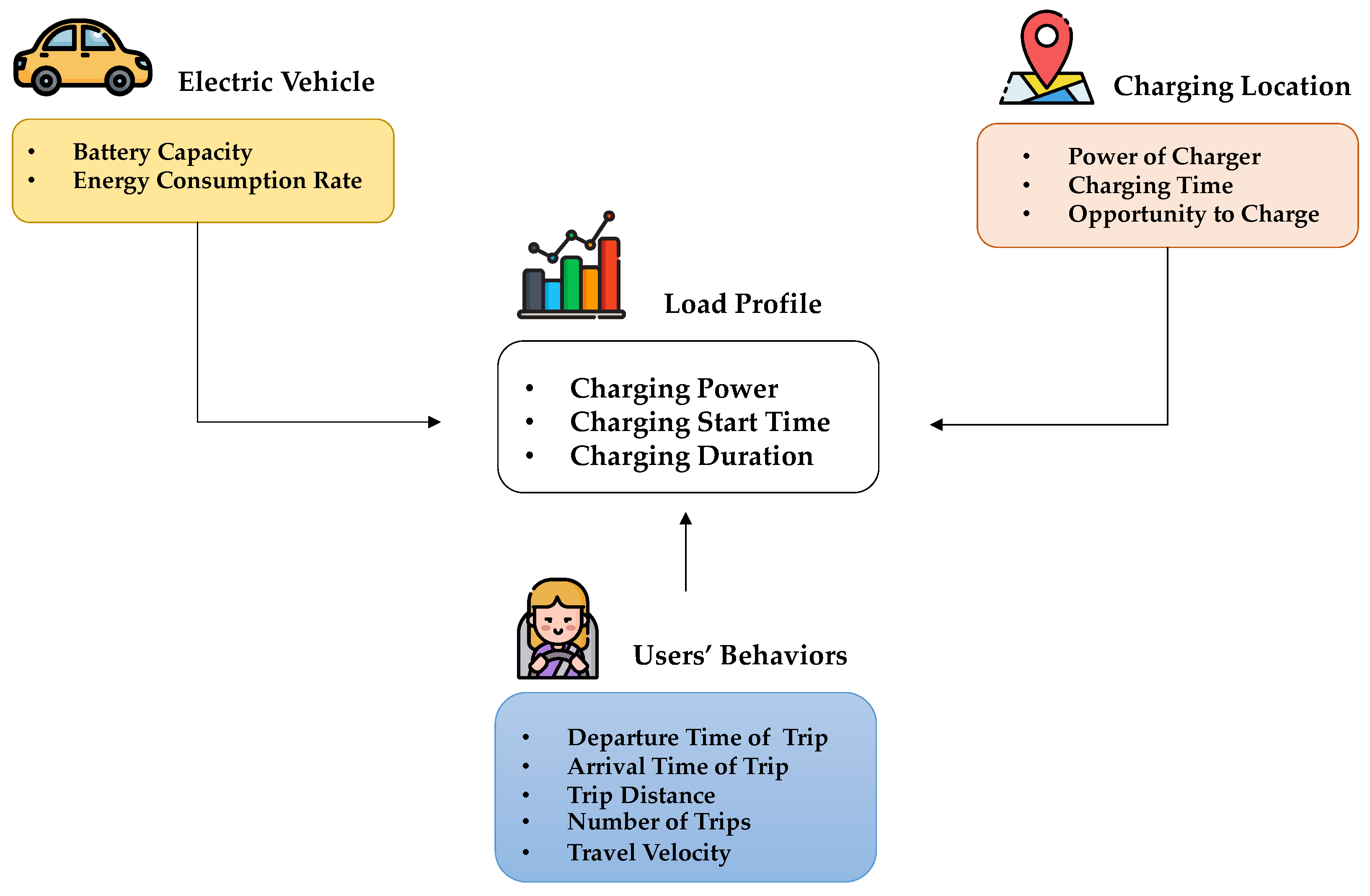
• The nature of EV loads can be movable around the system and time-dependent due to daily human activities; for example, users can charge their EVs at home in the evening, while the next day, they may recharge their EVs again at the workplace. Therefore, the EV loads can be moved around in the power system at different locations and times. These spatial effects were included in the load profile simulation and the optimization models developed in this research.
• A load profile simulation of the growing electricity demand from EVs was developed with two data sets: vehicle registration and a travel survey. The first set of data was used to formulate a density function of battery sizes of EVs on the market and obtained from the registration database of the Department of Land Transport (DLT), a government agency under the Ministry of Transport. The second set of data used for calculating the amount of electricity required to travel and to be recharged was obtained from the Office of Transport and Traffic Policy and Planning (OTP), a government agency under the Ministry of Transport, which conducted a travel demand survey of 18,833 house-holds in the city of Bangkok and neighboring provinces. The data obtained were statistically derived for giving the probability density functions of stochastic variables required in EV simulations, such as mileage driven, start charging time, departure time from homes, and the number of trips per day.
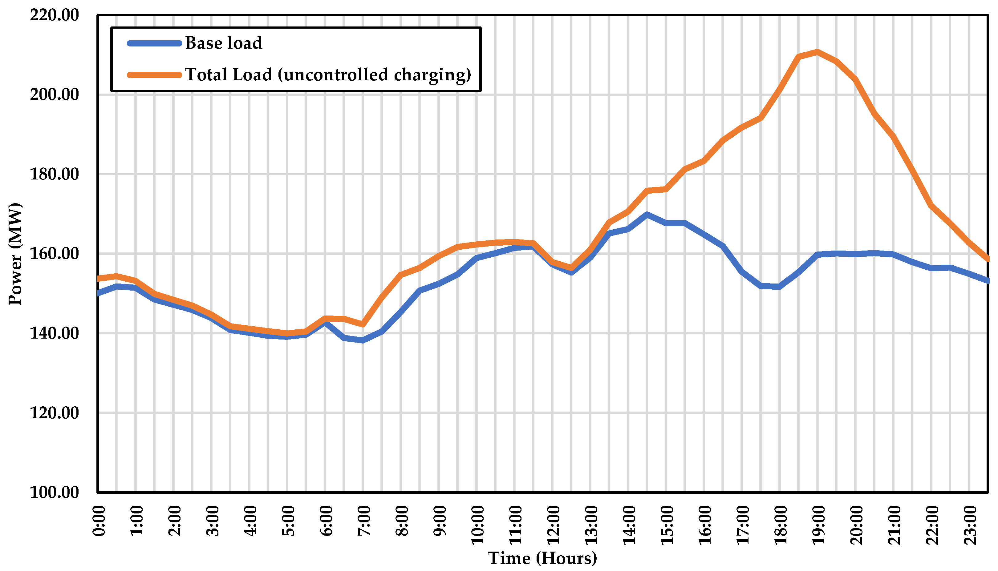
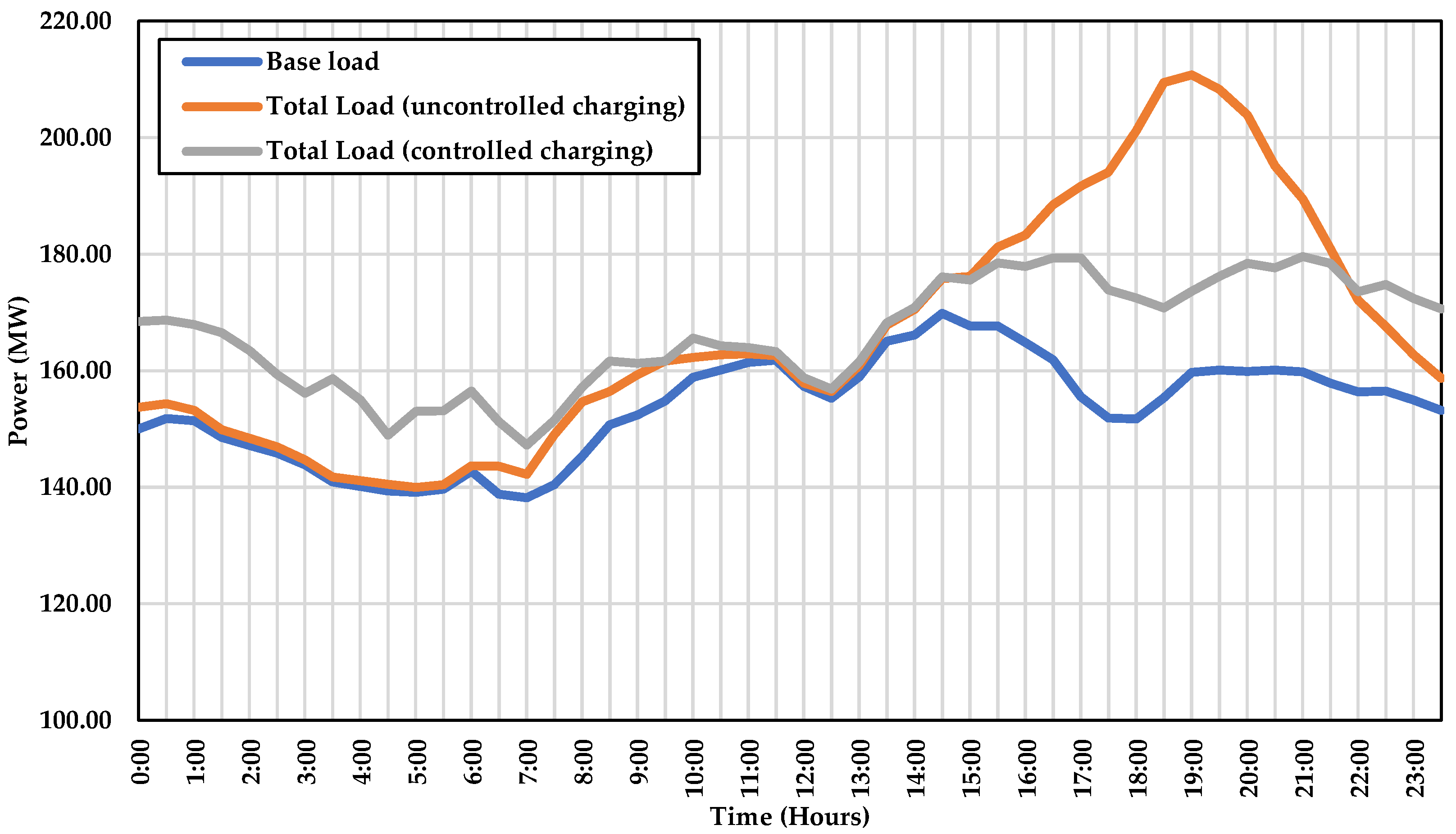
• Load profiles with uncontrolled charging (also known as dumb charging) were simulated with a behavior-based simulation with a number of EVs of 80,000. The simulation results of the charging demand of EVs reveal that the maximum demand would move from 2:30 p.m. to around 7:00 p.m., as most drivers return to their homes and recharge their EVs. Under the conditions of this study, the addition of EV demand could significantly lift the total peak load from 170 to 210 MW. This result can imply that higher levels of EV usage would lead to an outstanding increase in peak power demand and could directly impact the grid. Therefore, the rise of EVs would result in utilities having to invest in power system reinforcement to support the growing demand.
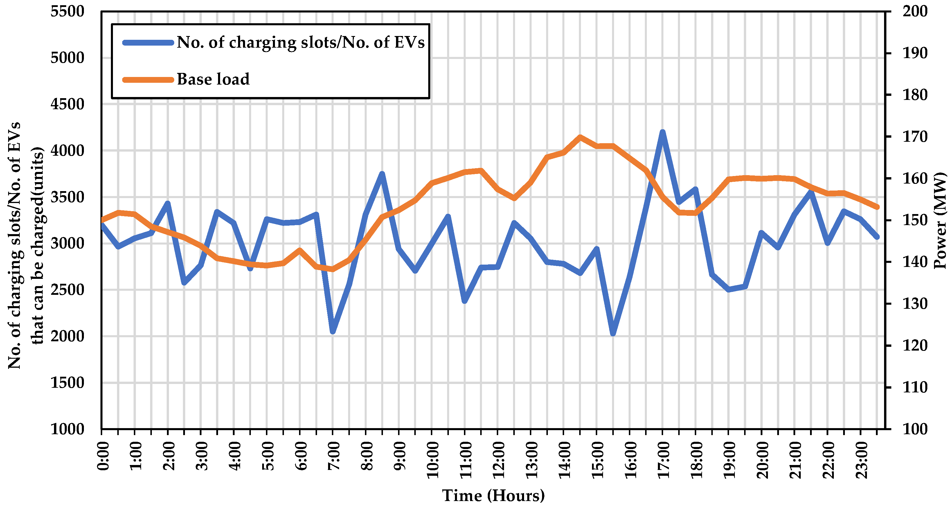
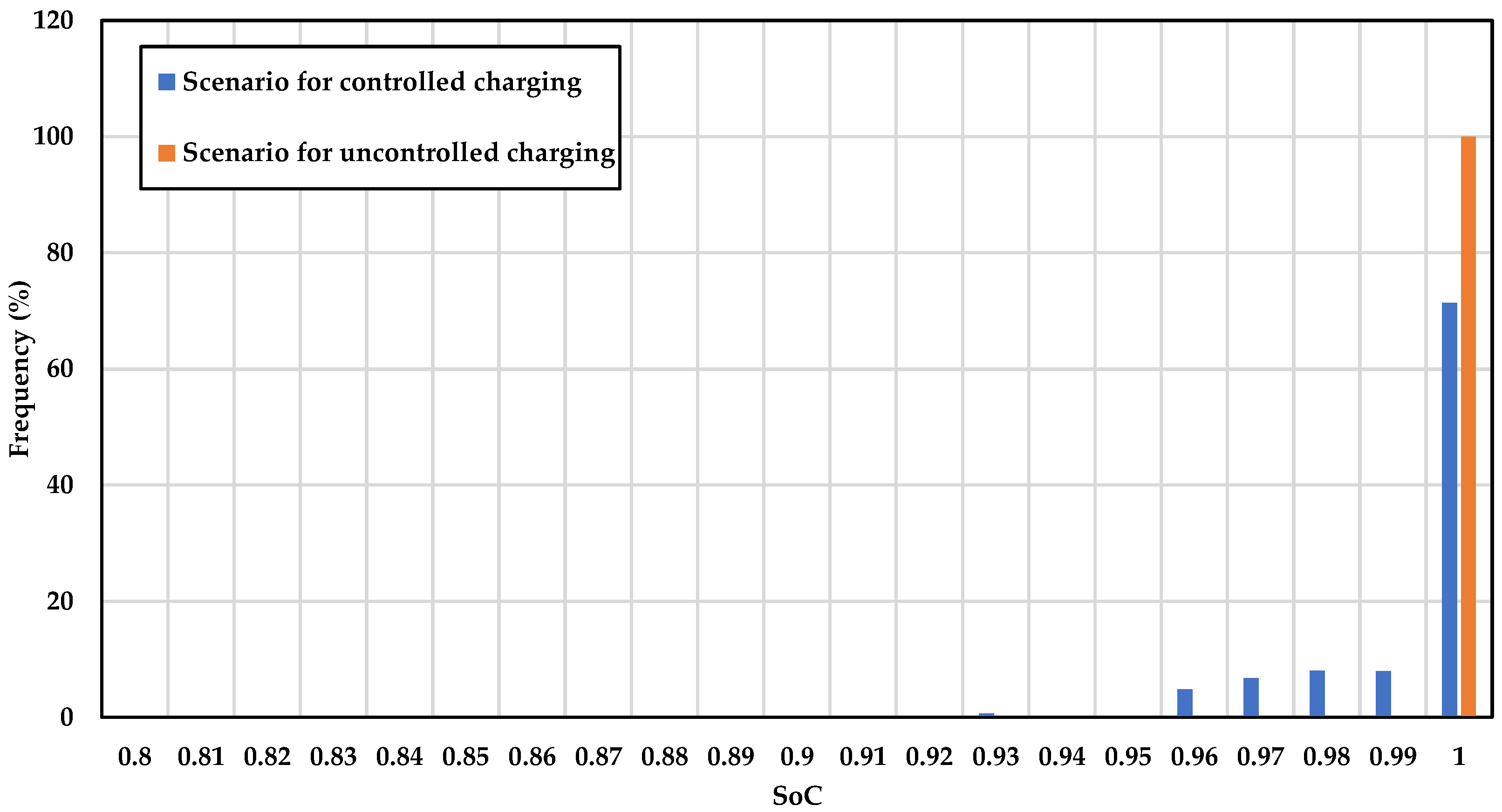
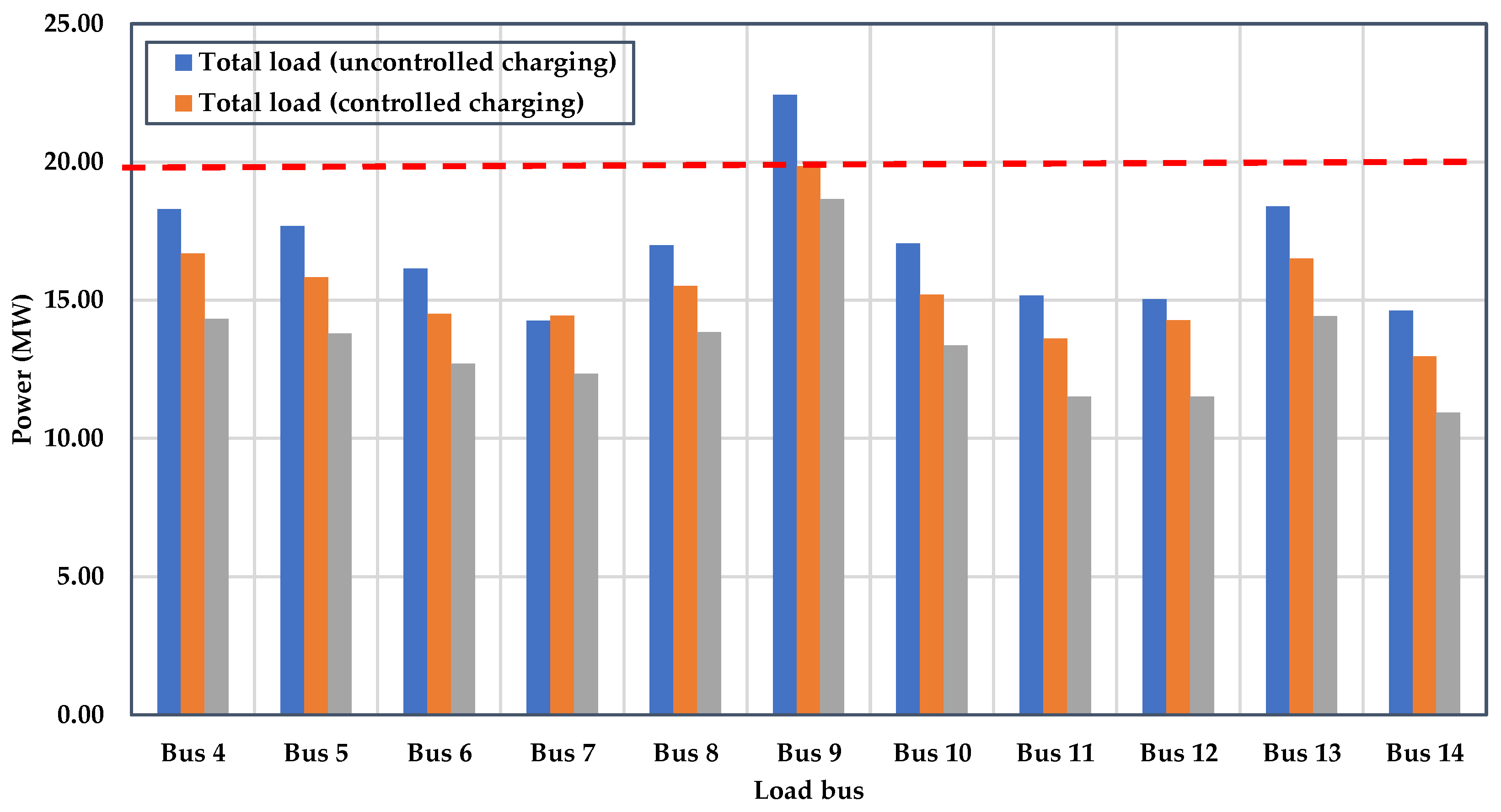
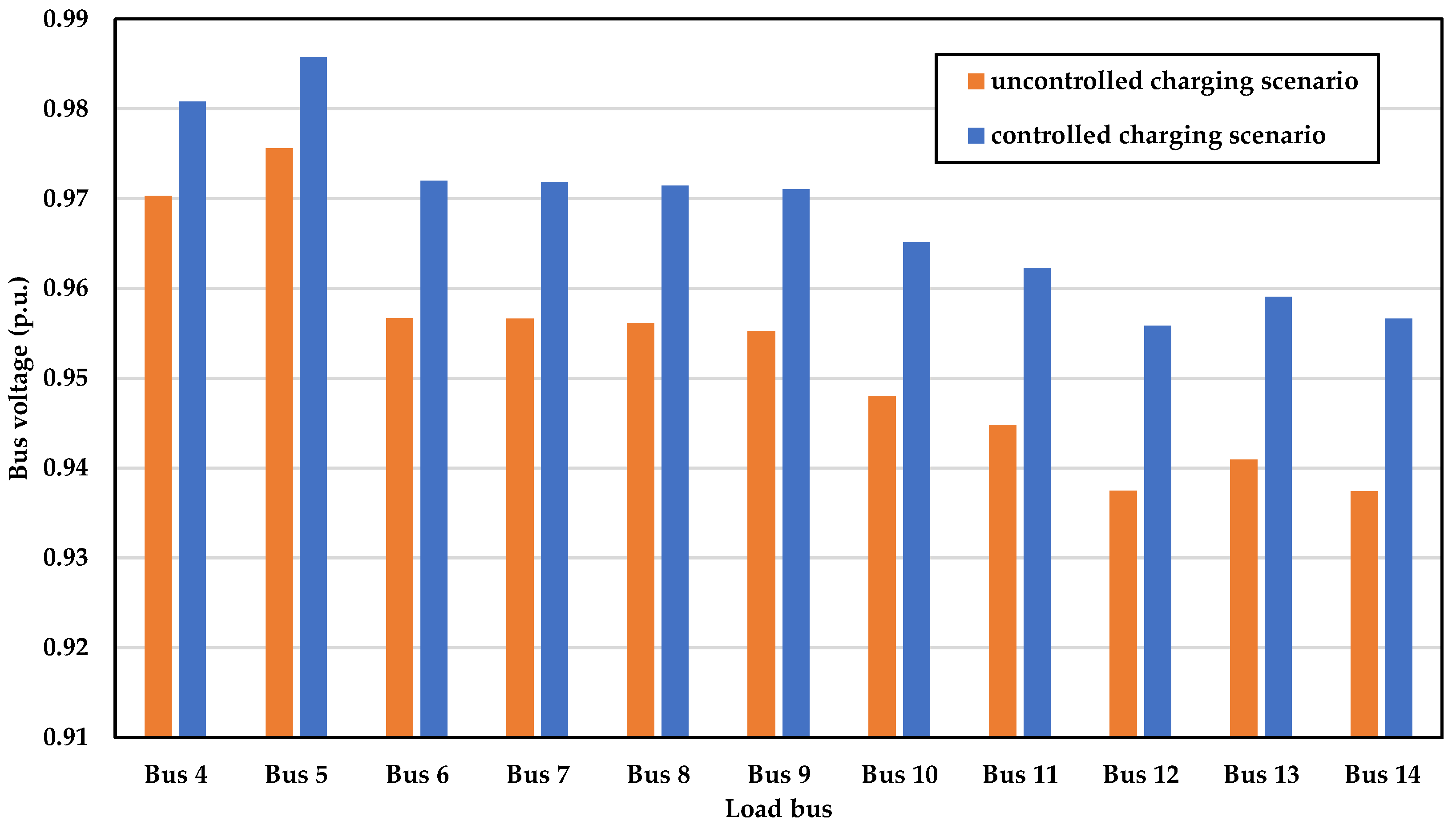
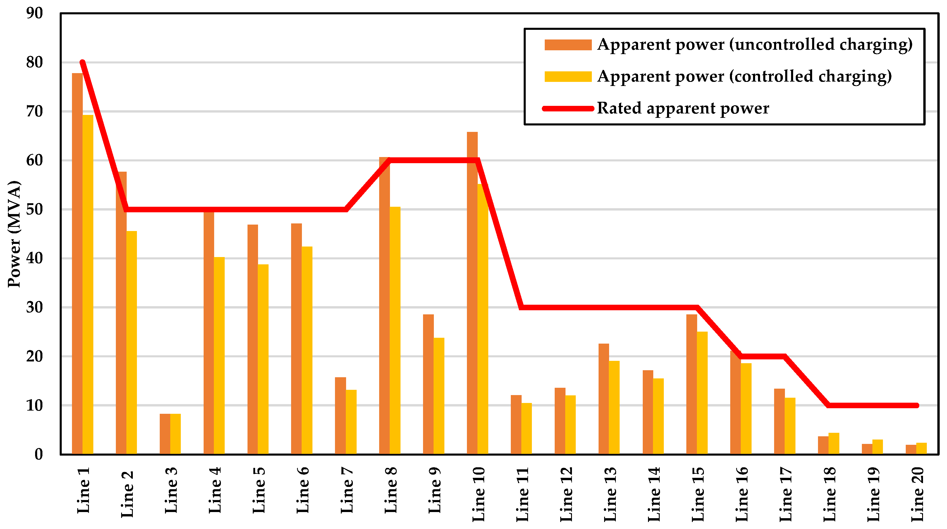
• A scheduling algorithm based on a genetic algorithm (GA) was proposed to define an optimal charging plan (properly available charging slots) in two domains: timeslots and locations. The scheduling algorithm operates along with charging event matrices to capture the charging events of all EVs, taking into account charging location, charging duration, parking duration, charging power, and start charging time. This set of metrics is updated each time EVs are charged. The algorithm can use these matrices as an input to simulate charging events and to define charging slots at each bus on each duration. The objective function of this algorithm is to maximize the system load factor and user satisfaction, subject to three operational constraints: bus voltages, bus powers, and line flow. After obtaining the optimal charging plan, EV queuing management was developed to select those qualified for each timeslot based on two indicators: previous charging duration and SoC. The test results from the modified IEEE 14 bus system can confirm the effectiveness of the developed GA.

3. Key Parameters of EV Modeling

3.1. EV Models

EVs are currently produced or imported into Thailand, and they come in a variety of brands and models. Because there are so many different brands and types of EVs, the characteristics of each model play a role in determining how people charge their cars.

The various types of EVs constitute essential factors that affect the charging patterns of EV users. Each type of EV model has a different battery size and energy consumption rate [17]. The different power consumption rates and battery sizes lead to different charging requirements in terms of charging duration and energy required.

Table 1. EV models are available in the Thailand market [18,19].

Model	Battery Size (kWh)	Energy Consumption Rate (kWh/km)	Market Share (%)
ZS EV	44.5	0.193	63.91
ONE	11.8	0.067	13.36
E6	80	0.260	5.34
LEAF	40	0.164	4.76
MODEL 3 PERFORMANCE	82.0	0.162	1.60
MODEL 3 LONG RANGE	75	0.154	1.51
E-TRON 55 Q	95	0.237	1.46
Others	-	-	8.06

shows the market share of EV models available in the Thailand market.

3.2. Types of Chargers

Another critical parameter that affects the charging power demand is the type of charger, each with a different range of power consumption. The study of [20] demonstrated that if EV owners were allowed to charge their EVs anytime and anywhere, the charging demand could increase the peak load at peak hours, the time at which users arrive at their destination. In addition, such an increased charging power resulted in shorter charging times, leading to increased load discontinuity. While there are many types of EV chargers available in the market, they can be broadly classified into three levels by the Society of Automotive Engineers (SAE) standard: AC Level 1, AC Level 2, and direct current fast charging (DCFC) Level 3. DCFC Level 3 is further divided into two sub-levels: DC Level 1 and DC Level 2. The detail of the charger standard based on the SAE is shown in

Table 2. Classification of chargers based on SAE J1772 standard.

Level	Charging Power (kW)	Location
Charging Level 1 (AC)	1.4–1.9 kW (single-phase)	Residential and Commercial building
Charging Level 2 (AC)	7.7–25.6 kW (single-phase/three-phase)	Private or Public
Charging Level 3 (DC Level 1)	13–39 kW (three-phase)	Public
Charging Level 3 (DC Level 2)	33–96 kW (three-phase)	Public

[10,21].

3.3. Driving Behaviors

Many studies have investigated the impact of users’ driving patterns on charging profiles and total charging demand. Reference [22] indicated that the charging pattern is based on user driving behaviors and vehicle performance, for example, the departure time and travel distance of the users. To reveal the relationship between energy needs and the behaviors of EV users, the study [23] showed that the minimum charging demand power period was around 4:00 a.m. according to the normal departure time, and the maximum peak time of residential charging demand was between 8:00 and 9:00 p.m., depending on connecting time and parking duration. The parking duration is purpose-specific, such as parking at the office during working hours, parking at home during night hours, and parking at a public charging station during charging. If an EV has been parked for a long period, it can be charged by using an AC Level 1 or an AC Level 2 charger to reduce the impact on the system [24]. The number of trips per day, trip distance, and travel velocity is other important parameters that influence the available time for charging and energy usage per day. The energy consumption, therefore, depends on charging duration and the remaining state of charge (SoC).

In this research, the driving style was determined using data from a driving behaviors study conducted in the city of Bangkok and surrounding areas by the OTP, and from [25]. The raw data were statistically examined and organized as the input data for EV driving and charging behaviors simulation, as shown in Figure 1. Five parameters could be derived from the survey consisting of the probability of the number of trips, velocity, distance per trip, departure time, and parking duration. It can be seen from Figure 1 that the number of trips is mostly two trips per day, and the average travel speeds are lower between 7 a.m. and 6 p.m. compared with other periods. Most of all the travel distances per trip did not exceed 10 km and the departure time of people is between 6 a.m. and 10 a.m. in the morning. The parking duration is divided into three cases depending on the number of trips. For the first trip, most parking durations are between 8–10 h, while the most likely parking duration stays within 4 h for second and third trips. It was also found that the everyday driving behaviors of personal vehicle users during weekdays are in the form of a roundtrip, people leaving their homes in the morning and returning home in the evening. Furthermore, more than 93% of roundtrips are a basic loop, which is a typical journey between two points, such as a roundtrip between home and workplace.

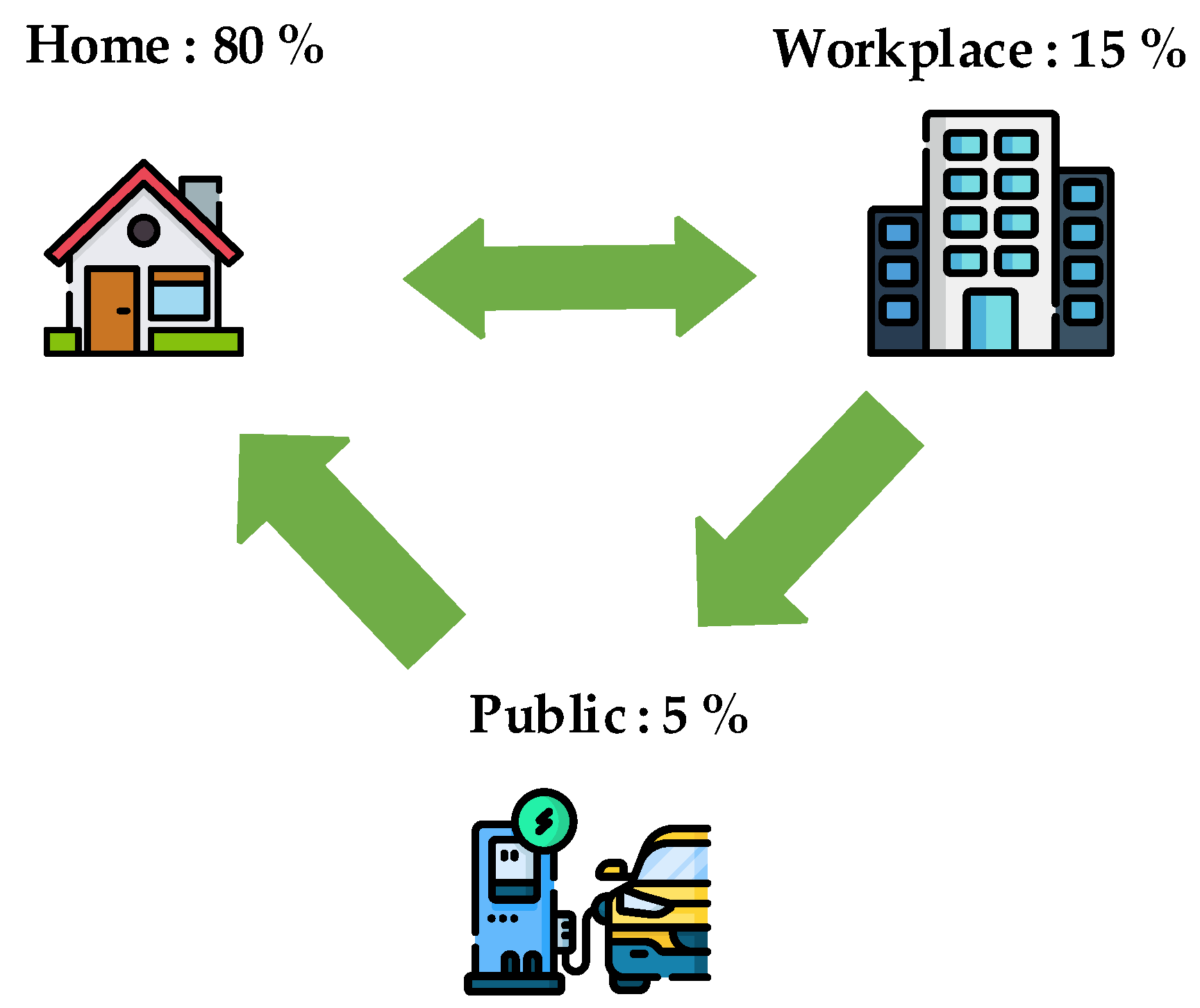
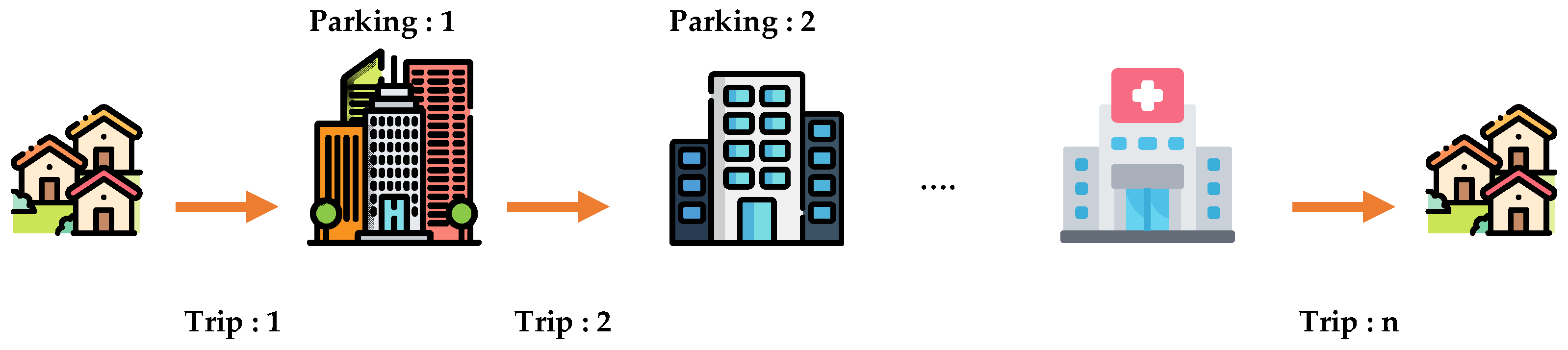
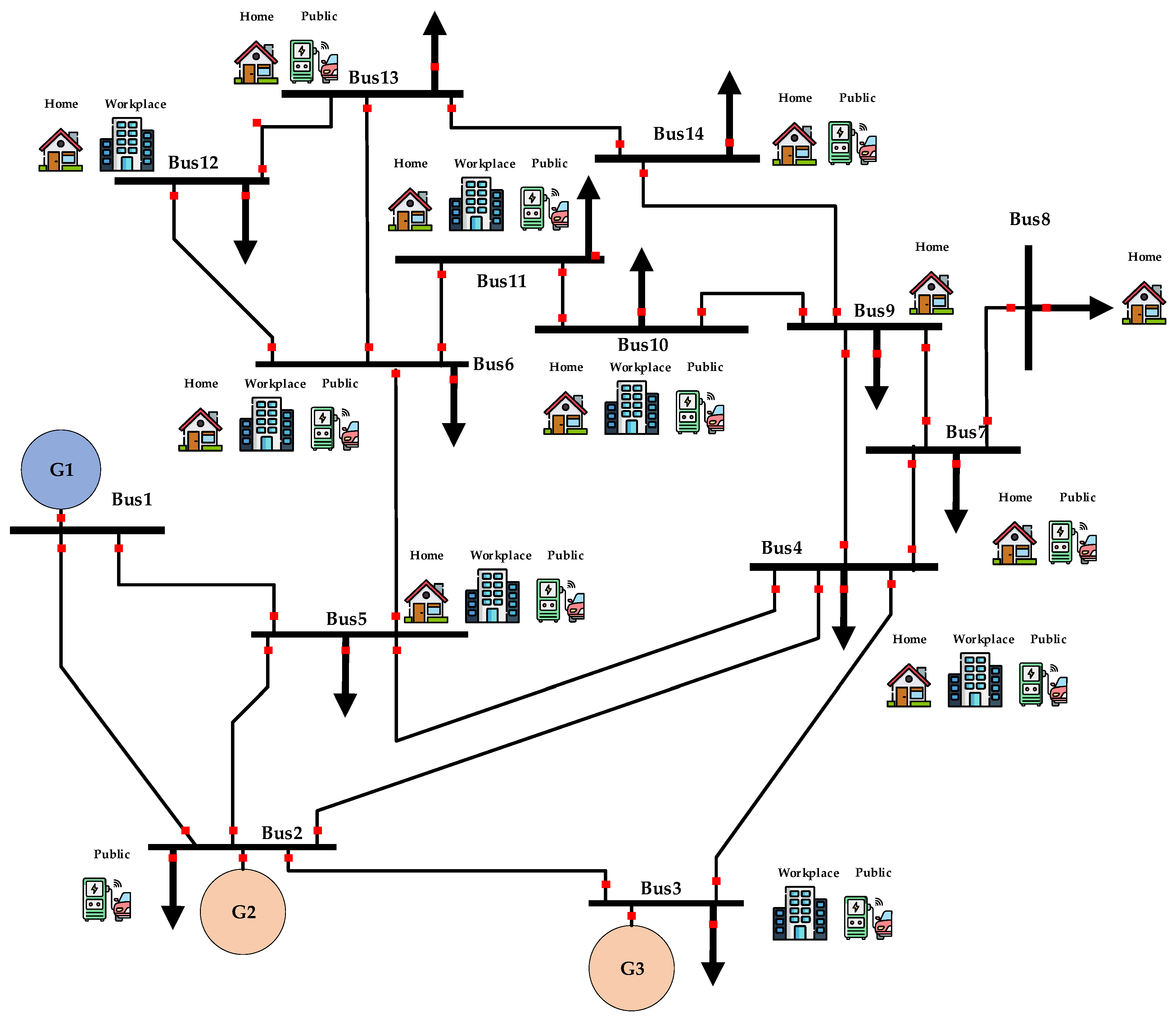
3.4. Charging Locations

EV users can choose their charging locations depending on satisfaction. They can charge their vehicles at work during working hours or at their homes/residencies during night hours. A charging station is one of the locations where users can charge their EVs while they are outside their homes. Many studies have investigated the charging probability of charging EVs at each location. For example, Ref. [26] presented a charging likelihood of 80% at homes/residents, 15% at workplaces, and 5% at public charging stations, as shown in Figure 2. Other research [27] also confirmed a similar proportion of charging. Due to users’ driving behaviors, most of them can generally charge EVs at home using AC chargers. Many research publications have indicated that users always start to charge their vehicles when they arrive at their destination immediately in the evening. In contrast, some users prefer to charge their EVs as soon as they arrive at their offices in the morning.

While home charging seems to have a typical pattern, charging EVs at public stations can occur at different times. For instance, the data collected from charging data in the UK [28] showed that low-power chargers were installed in public charging stations, and charging occurred from morning to afternoon while people were still working. However, other studies revealed that users in Denmark usually charged their EVs with DC chargers during peak hours after work due to the charging duration being shorter than AC chargers [29].

With the above charging behaviors, three possible charging sites with different likelihoods are of interest: approximately 80% at home, 15% at work, and 5% at public charging stations, as shown in Figure 2. In this research, we developed a behavior-based simulation algorithm to study the load profile of EV charging demand using driving behavior data. Three groups of input data, as shown in Figure 3, are required in the model: users’ behaviors, EV characteristics, and charging locations. With these input parameters, the load profile can be derived in the forms of charging power, charging start time, and charging duration.

4. Behavior-Based Charging Profile Simulation Algorithm

To analyze charging demand and to simulate uncontrolled charging conditions, this study used data combined from both survey and research publications. These stochastic data are used in our activity-based Monte Carlo simulation [30]. However, achieving an accurate analysis requires a thorough analysis of travel behavior together with an analysis of the efficiency of EVs. From the survey data, weekday driving patterns can be investigated with the assumption all drivers travel in the form of a trip chain [31]. In addition, the study found that most of them start traveling from their homes/residences in the morning and arrive home in the evening in the form of a round trip, as shown in Figure 4. Although the number of daily trips varies according to the behavior of each driver, the state of travel can be divided into two typical patterns: static and dynamic.

• Static state is the parking status of EVs. In this state, EVs can be charged or uncharged (idle) based on user decisions. When an EV is charged, it draws electrical power and energy from the network and increases the system load.
• The dynamic state is the mobility state in which EVs are moving from one location to another, meaning that battery power is consumed during the trips.

The algorithm for simulating an EV charging profile, which is a chronological variation in the EV power demand versus time, is detailed step-by-step in Algorithm 1 with the following conditions. EVs must be recharged daily, and the charging sites are randomly selected based on their likelihood, which is 80% at home, 15% at work, and 5% at public charging stations. The charging power ($P_j$) for each of these sites is respectively 7.7 kW ($P_1$), 22 kW ($P_2$), and 50 kW ($P_3$). Every trip is a round trip, namely starting from home in the morning and returning home in the evening, while there can be at least one parking place during the daily journey. The algorithm sequentially analyzes and simulates the driving behaviors of individual EVs at each timeslot.

Note that in step 6-2 of the algorithm, two options are selectable. In the first option, there is no centralized control over EVs charging scheduling technique. In this option, Algorithm 1 is simulated with a predefined number of iterations to find the possible maximum power demand for all timeslots and iterations according to (7). The daily load profile containing maximum peak demand can represent the worst possible case of uncontrolled charging and can serve as a benchmark for peak reduction in controlled load profiles as derived in Algorithms 2 and 3. The second option has a centralized control equipped with communication between EVs and the control center, which allocates individual EVs to be charged to each timeslot. Step 6-3 collects charging events to create the charging event matrices (detail given in Algorithm 2).

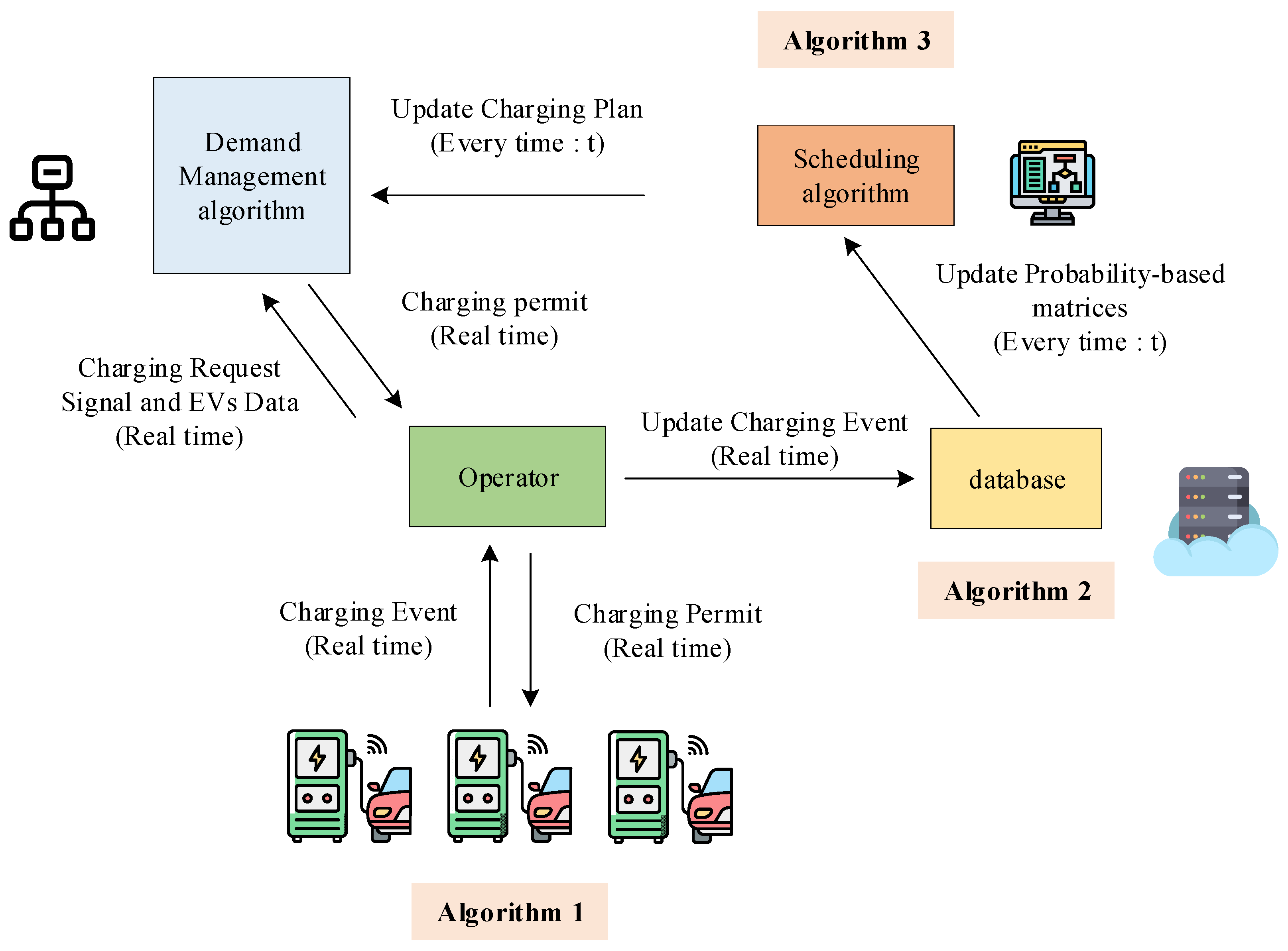
Algorithm 1: Pseudocode for behavior-based charging profile
Input	EVs parameters, driving behaviors data, number of EVs, and number of timeslots
Output	EVs charging profile at each location (i.e., each bus in the network) and power flow result at each timeslot
1	Create the characteristics of the EVs by Randomize the battery size, and energy consumption rate of each EV based on the model and market share as shown in Table 1 Randomize the initial location of EVs (i.e., always starting at home) at each bus on the system.
2	Randomize initial departure times ($t_i^{depart}$), next locations ($next\_lo{c}_i$) of EVs, and max trips per day of EVs ($tri{p}_i^{\max }$)
3	Set initial locations of all EVs at home ($lo{c}_i$), and $tri{p}_i=0$
4	Set all EVs statuses ($statu{s}_i=‘park’$)
5	Randomize initial charging locations ($c\_lo{c}_i$) of all EVs
6	For$t=1$ to $NTS$
6-1	For $i=1$ to $NEV$
6-1-1	IF $statu{s}_i=‘park’$ , and $t=t_i^{depart}$
6-1-1-1	$statu{s}_i=‘drive’$
6-1-1-2	Calculate $So{C}_i$, and $t_i^{arrive}$ by (1) and (2)
	ELSE IF $statu{s}_i=‘drive’$, and $t=t_i^{arrive}$
6-1-1-3	$statu{s}_i=‘park’$
6-1-1-4	$lo{c}_i=next\_lo{c}_i$
6-1-1-5	$tri{p}_i=tri{p}_i+1$
6-1-1-6	IF $tri{p}_i<tri{p}_i^{\max }$
6-1-1-6-1	Randomize $next\_lo{c}_i$, and parking duration ($\Delta t_i^{park}$)
6-1-1-6-2	Calculate $t_i^{depart}$ based on (3)
	ELSE
6-1-1-6-3	Randomize departure time ($t_i^{depart}$), next location ($next\_lo{c}_i$), and charging location ($c\_lo{c}_i$) for the next day
6-1-1-6-4	Set $tri{p}_i=0$
	END IF
	END IF
6-1-2	IF $statu{s}_i=‘park’$ and $So{C}_i<1$, and $lo{c}_i=c\_lo{c}_i$
6-1-2-1	$c\_statu{s}_i=1$ ($E{V}_i$ needs charging)
	ELSE
6-1-2-2	$c\_statu{s}_i=0$ ($E{V}_i$ is idle)
	END IF
	END FOR
6-2	Define charging permission of EVs ($pm\_statu{s}_i$)   •  For uncontrolled charging, all EVs are allowed to be charged and continue to Step 6-3   •  For controlled charging, only some of the EVs are allocated using the EV queuing management defined by Algorithm 3 then continue to Step 6-3
6-3	Collect EV charging events (refer to Algorithm 2)
6-4	For $i=1$ to $NEV$
6-4-1	IF $pm\_statu{s}_i=1$
6-4-1-1	Charge $E{V}_i$, and calculate $So{C}_i$ by (4)
6-4-1-2	Calculate the charging load at each location ($loa{d}_{b,t}$) by (5)
	END IF
	END FOR
6-5	Calculate total load ($loa{d}^{total}$) by (6)
6-6	Perform power flow analysis by the Newton–Raphson iterative algorithm [32]
	END FOR

Algorithm 2: Pseudocode for charging event matrices
Input	EV charging event data, number of EVs, and number of timeslots
Output	Charging event matrices
1	For$t=1$ to $NTS$
1-1	For $i=1$ to $NEV$
1-1-1	IF $c\_statu{s}_i=1$ and $c\_statu{s}_{i (t-1)}=0$
1-1-1-1	Collect charging event (${\gamma }_{b,j,t}$) along with location (bus $b$), charging power ($P_j$) and time ($t$) of $E{V}_i$
1-1-1-2	Calculate charging duration ($\Delta t_i^{chg}$) and parking duration ($\Delta t_i^{park}$) by (8) and (9) respectively
1-1-1-3	Store all charging event data (${\gamma }_{b,j,t}$, $\Delta t_i^{chg}$, $\Delta t_i^{park}$) of this event to the database
	END IF
	END FOR
	END FOR
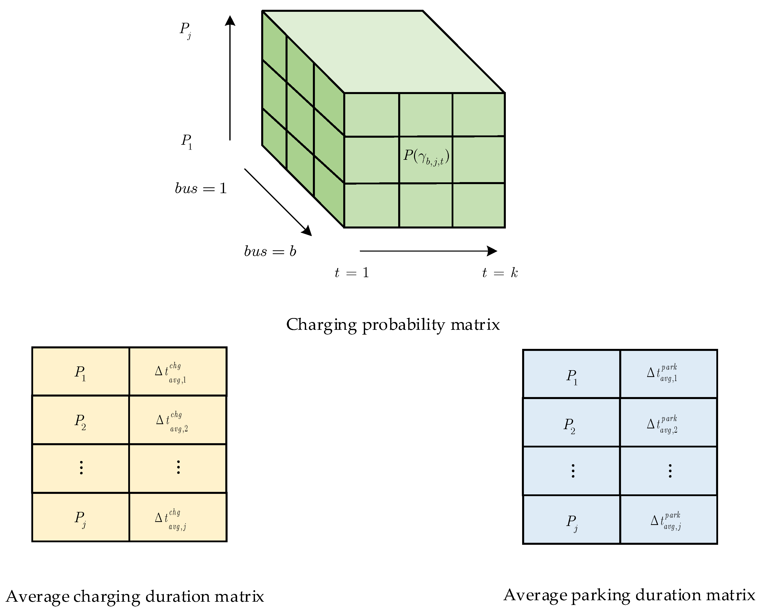
2	Calculate charging event matrices Calculate charging probability $(P({\gamma }_{b,j,t}))$ to obtain the charging probability matrix by (10) Calculate average charging duration $(\Delta t_{{}_{avg,j}}^{chg})$ to obtain the average charging duration matrix (11) Calculate average parking duration $(\Delta t_{avg,j}^{park})$ to obtain the average parking duration matrix (12)

Algorithm 3: Pseudocode for GA-based scheduling
Input	Charging event matrices, EVs, number of timeslots, number of chromosomes, and number of generations
Output	Charging plan (optimal charging slots at each timeslot)
1	Randomize initial values of first-generation chromosomes ${\left[\sigma \right]}_{b,t}$ (available charging slots)
2	For$iter=1$ to $NG$
2-2	For $p=1$ to $NC$
2-2-1	Create charging event characteristic of all EVs             •  Randomize charging location $(c\_lo{c}_i)$, power ($P_i$) and start time ($t_i^{start}$) based on the charging probability matrix             •  Determine the tentative charging duration of each EV $(\Delta t_i^{tent})$ and parking duration $(\Delta t_i^{park})$             •  Calculate available charging interval $[t_i^{start},t_i^{end}]$ using $\Delta t_i^{park}$ and $t_i^{start}$
2-2-2	For $t=1$ to $NTS$
2-2-2-1	For $i=1$ to $NEV$
2-2-2-1-1	IF $t\in [t_i^{start},t_i^{end}]$ and $\Delta t_i^{real}<\Delta t_i^{tent}$
2-2-2-1-1-1	$c\_statu{s}_i=1$ ($E{V}_i$ needs charging)
	ELSE
2-2-2-1-1-2	$c\_statu{s}_i=0$ ($E{V}_i$ is idle)
	END IF
	END FOR
2-2-2-2	Define charging permission of EVs ($pm\_statu{s}_i$) based on both the EV queuing management method and the available charging slots ${\left[\sigma \right]}_{b,t (p)}$
2-2-2-3	For $i=1$ to $NEV$
2-2-2-3-1	IF $pm\_statu{s}_i=1$
2-2-2-3-1-1	$\Delta t_i^{real}=\Delta t_i^{real}+1$
2-2-2-3-1-2	Calculate charging load ($loa{d}_{b,t}$) by (5)
	END IF
	END FOR
	END FOR
2-2-3	Calculate total load ($loa{d}^{total}$) by (6) and obtain maximum total load ($loa{d}_{total}^{\max }$)
2-2-4	Estimate preferred charging duration ($\Delta t_{total}^{pf}$) and controlled charging duration ($\Delta t_{total}^{ct}$) by (14) and (15)
2-2-5	Perform power flow analysis to obtain the peak power at each bus, and active and reactive power flow of each line
2-2-6	Apply a penalty constant (e.g., 106) for constraint violation in (16) to (18)
2-2-7	Evaluate the fitness of chromosome by (13)
	END FOR
2-3	Select and keep the best fitness from population
2-4	Bring population to the crossover, mutation process, and chromosome reproduction
	END FOR

$$So{C}_i=So{C}_i-\frac{D_i\times E_i}{B_i}; i=1 \mathrm{to} NEV$$

(1)

$$t_i^{arrive}=t_i^{depart}+\frac{D_i}{v_t}; i=1 \mathrm{to} NEV, t=t_i^{depart}$$

(2)

$$t_i^{depart}=t_i^{arrive}+\Delta t_i^{park}; i=1 \mathrm{to} NEV$$

(3)

$$So{C}_i=So{C}_i+\frac{P_i\times \Delta t^{slot}}{B_i}; i=1 \mathrm{to} NEV$$

(4)

$$loa{d}_{b,t}=loa{d}_{b,t}+P_i; t=1 \mathrm{to} NTS, b=1 \mathrm{to} NB$$

(5)

$$loa{d}^{total}={\displaystyle \sum _{b=1}^{NB}loa{d}_{b,t}}; t=1 \mathrm{to} NTS$$

(6)

$$loa{d}^{\max }=Max\left\{loa{d}_{iter}^{total}\right\}; iter=1 \mathrm{to} NI$$

(7)

5. Smart Charging by Direct Load Control Technique

Because charging EVs occur almost instantly upon arrival and frequently at the same time during peak power consumption, as a result, the charging during this time raises the peak power requirement dramatically. The difference between peak and off-peak powers may be so great that a management framework is required for connecting EVs to smart grid systems and allowing system operators and utilities to control charging demand [33]. EV charging regulation is frequently required by demand side management like peak load shaving, which helps both utilities and customers to narrow the gap between new and existing peaks. Centralized scheduling with unidirectional power flow is one of the charging control technologies whereby EVs can only receive power from the grid in one way [34]. In this technology, EVs are connected with utilities or aggregators, which collect information and control EV charging requirements. Algorithms are created to manage charging demand while keeping the peak as low as possible by allocating the appropriate number of EVs to be charged at each timeslot. For this type of control, an EV queuing management method is introduced in this paper for selecting proper EVs to be charged at each timeslot based on two qualification indicators: previous charging duration and SoC. This study also proposes charging event matrices and a GA-based scheduling algorithm which were developed for optimizing charging slots at each timeslot based on users’ behaviors.

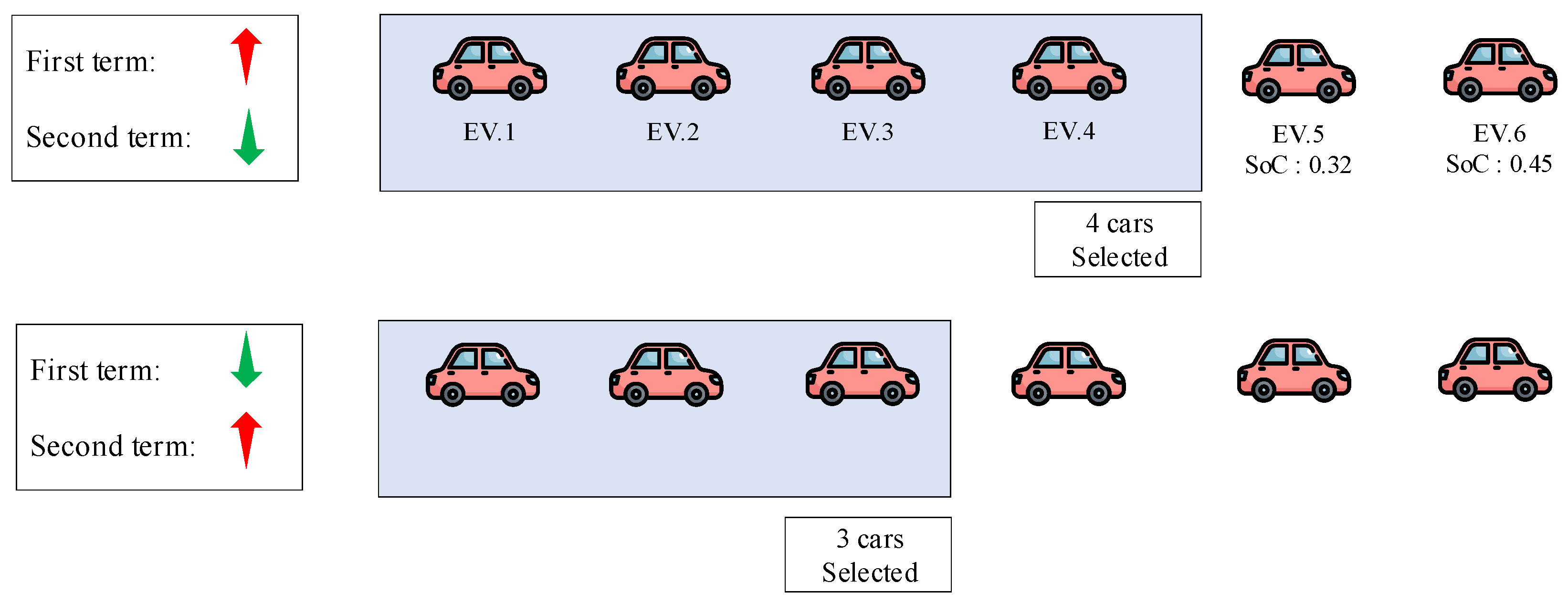
5.1. EV Queuing Management

For electric power utilities or demand management operators, selecting the correct and suitable EV to be able to be charged becomes essential, as it directly affects users’ satisfaction. Two useful indicators for selecting EVs are the previous charging duration and the remaining SoC received from each EV. This prioritization strategy is a straightforward and resource-saving method of fast computation.

One of the most effective algorithms for scheduling requirements is based on charging duration. Because it simply requires information regarding the charging duration of EVs, this method is practically simple and computationally fast to implement. In this strategy, it is reasonable to suppose that customers with longer charging periods already have a high SoC, whereas newcomers are expected to have a low SoC after their journeys. Some of the EVs that can be charged at any timeslot are strategically chosen based on how long they have been charged previously. As seen in Figure 5, their charging times are listed in ascending order. To enable the charging interchangeability of the EVs, this technique is repeated at each timeslot.

Charging management based on the SoC, alternatively, offers an innovative charging solution. The principal idea is that when an EV needs charging, it transmits a signal to the operator along with its charging information as in the previous technique. Suppose the system demand is surpassed in any timeslots. In that case, the operator can choose only a subset of the EVs that can be recharged based on their SoCs in ascending order, as depicted graphically in Figure 6. This process is recalculated at each timeslot.

5.2. Charging Slot Optimization by Genetic Algorithm

Although the direct charging control based on previous charging duration or SoC allows the system operator to systematically prioritize EVs, the maximum number of EVs (or the maximum available charging slots) that can be recharged at any given timeslot is another variable that needs to be set appropriately to attain the maximum peak reduction. This research proposes a GA-based scheduling algorithm to achieve this objective. However, because the GA is a time-consuming stochastic search, we have developed an improved mechanism for generating a proper input using charging event matrices, as shown in Algorithm 2. As the charging of EVs is an intertemporal process by which the system operator has to make decisions about how many and how long the EVs can be charged at various points in the timeslot, choices at one timeslot influence the availability at other timeslots. These charging event matrices can help solve this problem by estimating the likelihood of a charging pattern in each timeslot.

The algorithm stores EV charging data in different locations and times to create the charging event matrices, consisting of charging probability, average charging duration and average parking duration, as shown in Figure 7. These three matrices derived from Algorithm 2 will be applied to Algorithm 3 to define a proper charging plan. The charging probability matrix stores charging events at each bus with various charging powers over time for investigating the likelihood of charging events. It can be used as a guideline to forecast incoming charging demand. The average charging duration matrix operates with the charging probability matrix to capture the average charging duration at each power level. Likewise, the average parking duration matrix is similar to the average charging duration matrix in that it captures and analyzes the parking duration when users park and charge in each of three locations (i.e., workplace, public charging station, home). The advantage of the use of these three matrices is that they provide a convenient way to simulate charging behaviors in an area of interest.

$$\Delta t_i^{chg}=\frac{(1-So{C}_i)\times B_i}{P_i}; i=1 \mathrm{to} NEV$$

(8)

$$\Delta t_i^{park}=t_i^{depart}-t_i^{arrive}; i=1 \mathrm{to} NEV$$

(9)

$$P({\gamma }_{b,j,t})=\frac{{\gamma }_{b,j,t}}{{\displaystyle \sum _{z=1}^{NTS}{\displaystyle \sum _{y=1}^{NCP}{\displaystyle \sum _{x=1}^{NB}{\gamma }_{x,y,z}}}}}; b=1 \mathrm{to} NB, j=1 \mathrm{to} NCP, t=1 \mathrm{to} NTS$$

(10)

$$\Delta t_{{}_{avg,j}}^{chg}=\frac{{\displaystyle \sum _{i=1}^{NEV}\sum _{n=1}^{{NCE}_i}\Delta t_{i,n(y)}^{chg}}}{{\displaystyle \sum _{z=1}^{NTS}{\displaystyle \sum _{x=1}^{NB}{\gamma }_{x,y,z}}}}; y=P_j, j=1 \mathrm{to} NCP$$

(11)

$$\Delta t_{{}_{avg,j}}^{park}=\frac{{\displaystyle \sum _{i=1}^{NEV}\sum _{n=1}^{{NCE}_i}\Delta t_{i,n(y)}^{park}}}{{\displaystyle \sum _{z=1}^{NTS}{\displaystyle \sum _{x=1}^{NB}{\gamma }_{x,y,z}}}}; y=P_j, j=1 \mathrm{to} NCP$$

(12)

The objective function to be optimized by the GA, as shown in (13), consists of two terms, each attached with a weighted coefficient. The first term normalizes the maximum total load (load with EVs charging demand) by the maximum base load (load without EVs charging demand). The maximum total load ($loa{d}_{total}^{\max }$) can be obtained from a charging simulation in each chromosome, whereas the maximum base load ($loa{d}_{base}^{\max }$) is obtained from the actual original baseload. The second term represents user satisfaction calculated by comparing the preferred charging duration ($\Delta t_{total}^{pf}$) with the controlled charging duration ($\Delta t_{total}^{ct}$) obtained from the calculation process. To compute the maximum load, the preferred charging duration and the controlled charging, the charging event matrices is used as input data. The weighted coefficients (${\mu }_L,{\mu }_S$) determine the priority of each term, depending on whether the focus is on minimizing power demand or on maintaining user satisfaction. Both coefficients can be defined in the range [0, 1], and their summation equals to 1.

Objective function:

$$Min z = {\mu }_L\left(\frac{loa{d}_{total}^{\max }}{loa{d}_{base}^{\max }}\right)+{\mu }_S\left(\frac{\Delta t_{total}^{pf}}{\Delta t_{total}^{ct}}\right)$$

(13)

Subject to:

$$\Delta t_{total}^{pf}={\displaystyle \sum _{i=1}^{NEV}\Delta t_i^{tent}}$$

(14)

$$\Delta t_{total}^{ct}={\displaystyle \sum _{i=1}^{NEV}\Delta t_i^{real}}$$

(15)

$$V_b^l\le V_b\le V_b^u$$

(16)

$$p_b^l\le p_b\le p_b^u$$

(17)

$$s_l^l\le s_l\le s_l^u$$

(18)

To find an optimal solution of (13), we introduce chromosome ${\left[\sigma \right]}_{b,t}$, the structure of which is a matrix with a dimension of $b\times t$ and represents the available charging slots bus $b$ and time $t$. A high availability of charging slots in each timeslot will increase the first term and decreases the second term of the objective function. Conversely, when the number of available charging slots becomes limited, the value of the first term decreases while the second term will increase as shown in Figure 8. Nevertheless, if the fitness variable is properly configured, the value of the first term will decrease with little effect on the second term. This will cause the charge of EVs to be distributed over time, and the charging event will occur during the off-peak period while maintaining user satisfaction.

The objective function of the scheduling algorithm is subject to three constraints. First, the system operator must maintain the voltage magnitudes at all buses within prespecified limits expressed by (16). Second, the active power of all load buses must be maintained within a permissible value given by (17). Third, the power flow on the lines must not exceed their loading capability limits expressed by (18). The variables $V_b, p_b$ and $s_l$ are determined from power flow computation [32].

The process of the GA basically contains three main operators: chromosome reproduction, crossovers, and mutations for diversity [35], as shown in Algorithm 3. The procedure starts with the generation of a random population of chromosomes that represent possible solutions to the problem. Each solution is assessed based on measurable criteria, with each chromosome receiving a fitness score. To calculate the fitness of each chromosome that represents available charging slots, three main steps are required.

In the first step, the charging event matrices are used to randomize charging events of the existing number of EVs to obtain their charging locations, charging powers, and plug-in times. The tentative charging duration ($\Delta t_i^{tent}$) and the parking duration ($\Delta t_i^{park}$) of each EV are determined from the charging power using the average charging duration matrix and the average parking duration matrix.

In the second step, the charging demand profile of each chromosome is calculated by utilizing the charging events obtained from the first step and the available charging slots of each chromosome. The controlled charging duration $\Delta t_{total}^{ct}$ is obtained by counting the real charging duration ($\Delta t_i^{real}$), and the preferred charging duration $\Delta t_{total}^{pf}$ by the summation of $\Delta t_i^{tent}$. The charging load profile of this chromosome is then combined with the original baseload to give the total maximum demand ($loa{d}_{total}^{\max }$).

In the final step, the power flow calculation is performed to determine the fitness of the chromosome. If any the constraint violation is detected, a penalty is applied to this chromosome in the fitness evaluation. These three steps are repeated for all chromosomes in this generation. The second population (i.e., second-generation) is generated from the first population using the crossover and mutation processes. The GA search is terminated until the final generation has been reached. The best solution among all the generations is considered, as the optimal solution.

Figure 9 gives an overview of the coordination among the proposed three algorithms together with the EV queuing management module. The scheduling algorithm (Algorithm 3) can update the number of available slots ranging from every day to every hour in advance, which is suitable for day-ahead or intraday electric market trading. However, the charging plan can be updated more frequently, depending on the computational capacity of the computer device. For practical implementation of the operational process, when EVs are required to recharge their batteries, a signal will be sent to the operator and stored in the database to update the charging event matrices in real-time by Algorithm 2. The operator sends all charging requests along with the required data at each timeslot to the EV queuing management algorithm, which obtains the number of chargeable EVs at each timeslot from the scheduling algorithm, which performs the optimization procedure based on the updated charging event matrices. For this study, we would like to simulate the driving behaviors of EVs to analyze the shape of load profiles and to study the algorithms’ capability in controlling EV charging and scheduling the corresponding charging slots. For this reason, Algorithm 1 is served as a platform to simulate charging behaviors instead of obtaining the actual charging request as in real applications.

6. Case Study

The developed algorithms were tested with the modified IEEE-14 bus consisting of 3 generators and 20 transmission lines as shown in Figure 10. The generator data, and the transmission line data are shown in

Table 3. Generator data.

Generator No.	Bus	Type	Voltage (pu.)	Power (MW)
1	1	Slack	1.01	-
2	2	PV	1.01	55
3	3	PV	1.01	55

and

Table 4. Line data.

Line No.	From Bus	To Bus	Resistance (ohm)	Reactance (ohm)	Line Limit (MVA)
1	1	2	0.04	0.11	80
2	1	5	0.10	0.42	50
3	2	3	0.09	0.38	50
4	2	4	0.11	0.34	50
5	2	5	0.11	0.33	50
6	3	4	0.13	0.33	50
7	4	5	0.03	0.08	50
8	4	7	0.00	0.40	60
9	4	9	0.00	1.06	60
10	5	6	0.00	0.48	60
11	6	11	0.18	0.38	30
12	6	12	0.23	0.49	30
13	6	13	0.13	0.25	30
14	7	8	0.00	0.34	30
15	7	9	0.00	0.21	30
16	9	10	0.06	0.16	20
17	9	14	0.24	0.51	20
18	10	11	0.16	0.37	10
19	12	13	0.42	0.38	10
20	13	14	0.33	0.66	10

respectively. The system base voltage, and power are 13.8 kV and 100 MVA. It is assumed that at least one of the three charging locations (i.e., home, workplace, and public station) are placed at each bus as shown in Figure 10. The voltage at each bus must be maintained between 0.95 and 1.00 p.u.

It is also assumed that there are 80,000 EVs scattering over the system, and the initial load profile without this number of EVs is shown in Figure 11. The system has an initial load factor of 0.9, and the total maximum load is 170 MW at 2:30 p.m. When including the additional loads of the EVs, the load profiles of each bus are shown in Figure 12, and it is evident that the system has seen a sharp increase in power demand during the evening hours when most EV users return to their residences and charge their cars. As a result, the peak power demand in the system is increased to 210.67 MW, as shown in Figure 13 (about 40 MW increase from the initial system peak demand) and shifted from 2:30 p.m. to 7:00 p.m. However, because some buses do not have residential customers—for example, Bus 3, where there are only office buildings and charging stations nearby—the charging demand stays the same during the evening hours. Instead, the increased demand can be observed during the morning hours between 6:00–11:00 a.m. when people start arriving at their offices.

For the EV queuing management, the charging of EVs is arranged either based on their previous charging durations or the remaining SoCs, depending on the operator’s preference. Although the overall effect of using both indicators is the same, and improper allocation of charging timeslots to EVs can cause their SoCs to be lower than the users’ expectation, as shown in Figure 14. The figure shows that without control, an EV would be fully charged within 6 h (between 0:00 a.m.–6:00 a.m.). With an unsuitable control, it is possible that the vehicle might be forced to start and stop charging at certain intervals (e.g., four stops with different waiting times as shown in the figure) and therefore the SoC could be below the user’s expectation. Alternatively, a more suitable control could be to stop charging at 3:00 a.m. and to continue recharging at 5:00 a.m. in order to reach the users’ satisfaction before they leave home the next morning.

The scheduling algorithm was applied to define an optimal charging plan with weight coefficient, ${\mu }_L$= 0.8 and ${\mu }_S$= 0.2. In the GA process, the number of chromosomes and generations were respectively set at 300 and 40 with a uniform crossover rate of 0.3 and a mutation rate of 0.2. Figure 15 shows a comparison between the number of charging slots (namely, the number of EVs that can be charged) and the base load. It is obvious that the trend of the number of charging slots and the base loads move in opposite directions. In other words, when the baseload rose around from 2:00 p.m. to 11:00 p.m., the algorithm would try to reduce charging timeslots to mitigate the peak demand and maintain power at the proper level.

The results of the GA-based scheduling algorithm are shown in Figure 16, which shows the load profile in the case of controlled charging. Compared to the other scenario, the increase in power levels during the evening hours of mass charging of EV users is noticeably reduced due to the control algorithm that distributes the charging demand over time. As a result, many EV chargers are forced to delay starting charging during the low power demand of baseload. Considering the efficiency of the algorithm for controlling the charging of EVs, we find that the total maximum power demand is reduced to 179.56 MW, a 14.79% reduction from the uncontrolled charging peak power. The peak demand for controlled charging is slightly higher than the existing peak of the baseload at around 9.7 MW.

It is possible that the algorithm can cause dissatisfaction among EV users due to inadequate charging. For this reason, the EVs’ SoC must be compared after they have been charged before the next trip in both scenarios, as shown in Figure 17. The figure compares the distribution frequency of the SoC level before the EVs leave their homes between controlled and uncontrolled scenarios. It is very interesting to note that almost all of the users in the uncontrolled scenario can have their EVs fully charged, while about 70% in the controlled scenario can achieve this feature. However, full user satisfaction comes at the expense of a 40 MW increase in the system’s peak demand. Note that it would be worth doing this, as over 99% of EVs have a minimum SoC of 0.96 in the controlled scenario, which should be more than enough for the users to make a daily round trip.

In addition, if we wish to set the maximum power limit of each bus below 20 MW, the simulation result is shown in Figure 18. When analyzing each bus individually by comparing the maximum power demand at the load buses, we can observe that the maximum power demand at each bus in the controlled scenario is significantly lower than in the uncontrolled scenario. If users can charge their EVs independently, it would make the peak power demand on Bus 9 22.75 MW compared to 19.92 MW in the case of smart charging with direct load control. This can confirm that the developed algorithm can help the operator and utility to prevent a negative impact from the EV charging demand.

Figure 19 shows the daily voltage profile of each bus. At 7:00 p.m., the time at which charging a large number of EVs occurs simultaneously, the bus voltage drops sharply to as low as 0.937 p.u. at Bus 14. Buses 10–14 suffer a severe low voltage below 0.95 p.u. To alleviate this impact, the proposed algorithm not only managed to flatten the daily load profile but also kept all the bus voltages above 0.95 p.u., as shown in Figure 20. The comparison of the lowest bus voltage magnitude in each scenario is shown in Figure 21, demonstrating that the controlled charging scenario can completely mitigate the effect of voltage drop significantly.

The line flows are expected to increase for extensive use of EVs, as can be seen in Figure 22. In the uncontrolled scenario, most of the line flows still stay within their rated capacities, except for Line No. 2, 8, and 10. Line No. 2 is slightly overloaded, carrying 57.47 MVA, whereas Line 8 marginally exceeds 60 MVA by 0.49 MVA. Line No. 10 has seen its rated capacity of 60 MVA violated. Such overload problems can be prevented by the proposed algorithm (see Figure 22), which successfully managed to keep all the flows on the lines within their rated capacities.

Table 5. Performance comparison between uncontrolled charging and controlled charging.

	Uncontrolled Charging	Controlled Charging	Difference
Peak power demand (MW)	210.74	179.56	14.79%
Load factor	0.79	0.93	17.35%
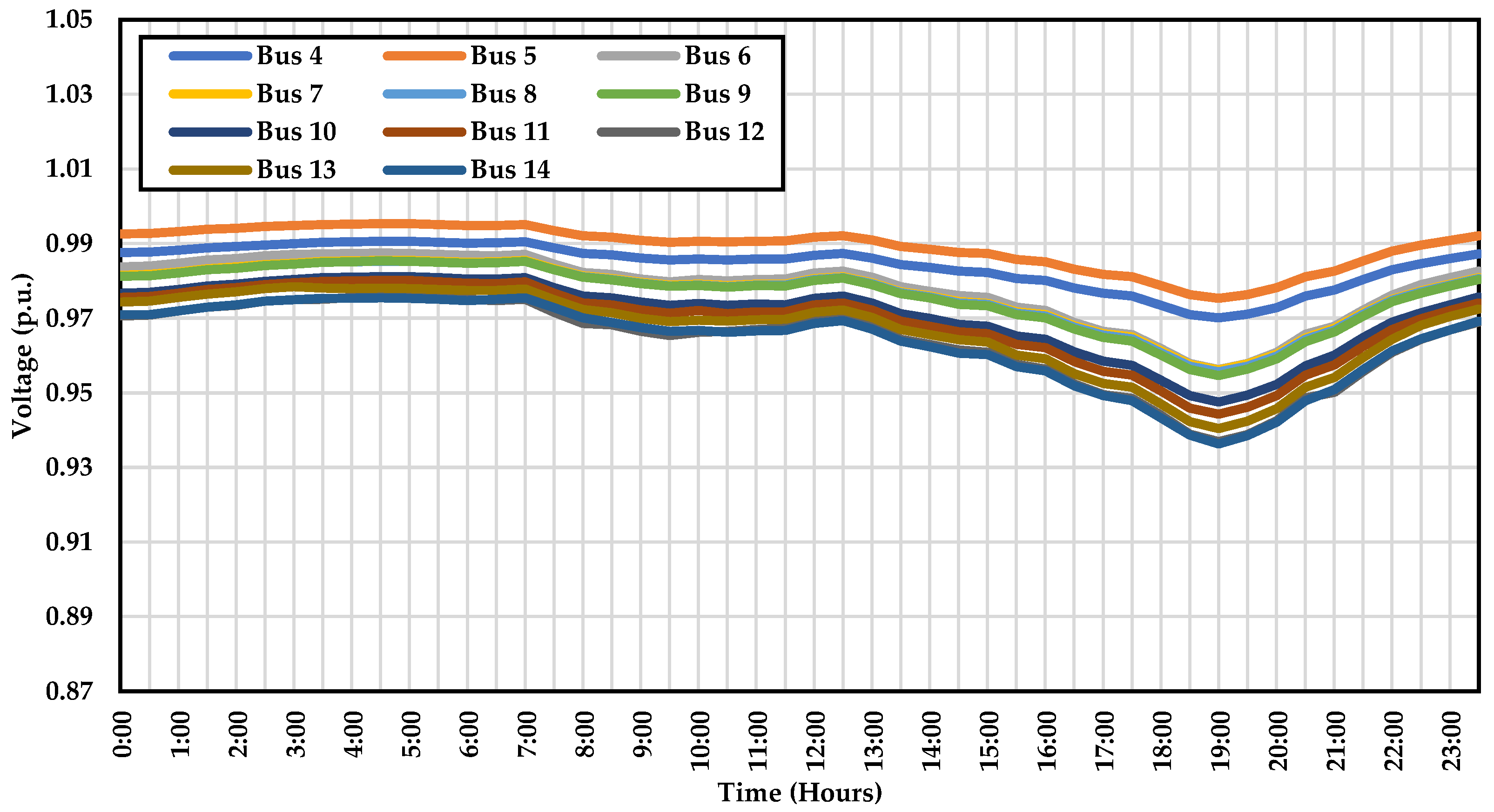
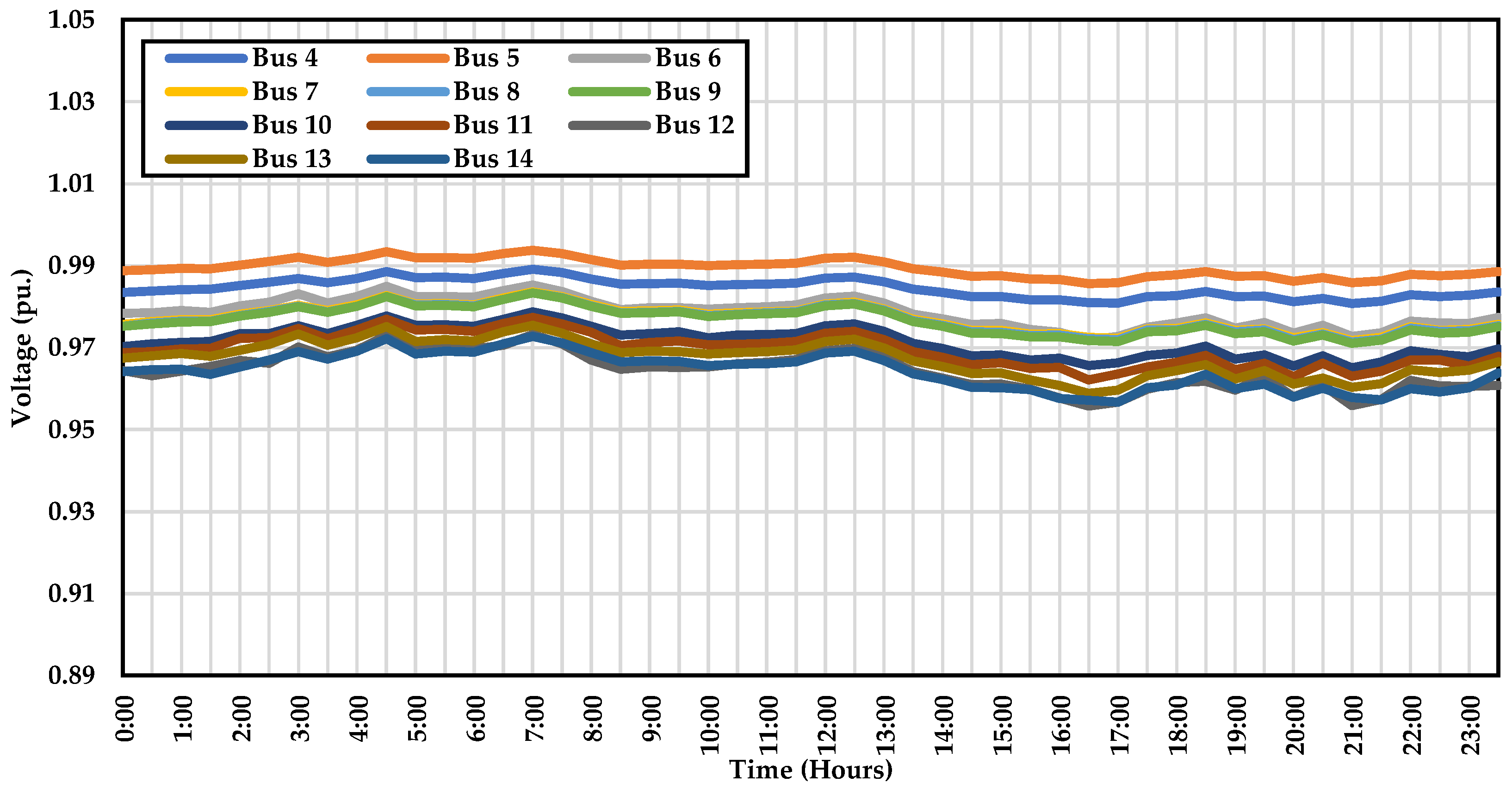
Maximum voltage drop (p.u.)	0.937	0.956	1.96%
Charging energy (MWh)	304.78	304.26	0.17%
Energy loss (MWh)	119.85	116.92	2.44%

compares the system performance between the uncontrolled scenario and the control scenario. The benefits of the proposed algorithms for load balancing and peak saving are obvious for better utilization of electrical energy and for reducing the peak load demand. First and most importantly, the system peak demand is approximately a 14.79% reduction, and the system load factor is significantly improved by 17.35%. Additional generation and transmission capacity investment could be significantly avoided. Second, the total energy consumption in the controlled charging is slightly lower because some EVs were charged during the period of low demand, for example, during the daytime. Although about 29% of the cars are not fully charged, almost all of their SoC are well above 0.96.

Finally, the energy loss is reduced by about 2.92 MWh per day. According to [36], the cost of electricity generation and transmission in Thailand is 2.86 Baht/kWh. If this amount of energy savings were the same for every day in a year, we would save 3,048,188 Baht a year (equivalently about $89,652 a year).

7. Conclusions

This paper has presented a comprehensive stochastic model to simulate movable EV charging patterns based on the driving behaviors and the performance of EVs. The behavior-based charging profile simulation can generate travel patterns and charging demand from multi-locations at different times of the day and give the spatial impact on the peak power demand caused by the widespread use of EVs in the sample area. To mitigate the negative impact from the rise of power demand, this study has introduced EV charging scheduling using the GA and EV queuing management algorithm. The former was used to define properly available charging slots of each bus at each timeslot in order to try to minimize charging peak demand while respecting the system operational constraints and maintaining user satisfaction. The EV queuing management algorithm intelligently identified successful EV candidates in the available slots based on previous charging durations and the remaining state of charge (SoC). The results of the modified IEEE 14 bus system results confirm that the developed methodology can efficiently manage the peak power demand while respecting the system operational constraints and retaining the user satisfaction level. The benefit of smart charging in terms of financial savings and the deferral of infrastructure reinforcement would be very significant for a practical-sized power system with a large number of EVs. The proposed methodology can be extended to include, for example, a more comprehensive scheduling algorithm to gain the ability to accommodate vehicle-to-grid (V2G) functions at specified intervals to support the grid, dynamic pricing schemes to convince users of EVs for a specific period of time, and integration of energy storage and renewable energy.

References

- Ehsani, M.; Singh, K.V.; Bansal, H.O.; Mehrjardi, R.T. State of the art and trends in electric and hybrid electric vehicles. Proc. IEEE 2021, 109, 967–984. [Google Scholar] [CrossRef]
- Parajuly, K.; Ternald, D.; Kuehr, R. The Future of Electric Vehicles and Material Resources: A Foresight Brief; UNU/UNITAR-SCYCLE: Bonn, Germany; UNEP-IETC: Osaka, Japan, 2020. [Google Scholar]
- Barkenbus, J. Prospects for Electric Vehicles. Sustainability 2020, 12, 5813. [Google Scholar] [CrossRef]
- Dharmakeerthi, C.H.; Mithulananthan, N.; Saha, T.K. Overview of the impacts of plug-in electric vehicles on the power grid. In Proceedings of the IEEE PES Innovative Smart Grid Technologies, Perth, Australia, 13–16 November 2011; pp. 1–8. [Google Scholar] [CrossRef]
- McCarthy, D.; Wolfs, P. The HV system impacts of large scale electric vehicle deployments in a metropolitan area. In Proceedings of the 20th Australasian Universities Power Engineering Conference, New York, NY, USA, 5–8 December 2010; pp. 1–6. [Google Scholar]
- Ni, X.; Lo, K.L. A methodology to model daily charging load in the EV charging stations based on Monte Carlo simulation. In Proceedings of the 2020 International Conference on Smart Grid and Clean Energy Technologies (ICSGCE), Kuching, Malaysia, 4–7 October 2020. [Google Scholar] [CrossRef]
- Ramadan, H.; Ali, A.; Farkas, C. Assessment of plug-in electric vehicles charging impacts on residential low voltage distribution grid in Hungary. In Proceedings of the 2018 6th International Istanbul Smart Grids and Cities Congress and Fair, ICSG 2018, Istanbul, Turkey, 25–26 April 2018; Institute of Electrical and Electronics Engineers Inc.: Piscataway, NJ, USA, 2018; pp. 105–109. [Google Scholar] [CrossRef]
- Liu, D.; Li, Z.; Jiang, J.; Cheng, X.; Wu, G. Electric Vehicle Load Forecast Based on Monte Carlo Algorithm. In Proceedings of the 2020 IEEE 9th Joint International Information Technology and Artificial Intelligence Conference (ITAIC), Chongqing, China, 11–13 December 2020; pp. 1760–1763. [Google Scholar] [CrossRef]
- Liu, Z.; Xie, Y.; Feng, D.; Zhou, Y.; Shi, S.; Fang, C. Load forecasting model and day-ahead operation strategy for city-located EV quick charge stations. In Proceedings of the 8th Renewable Power Generation Conference (RPG 2019), Shanghai, China, 24–25 October 2019; pp. 1–6. [Google Scholar] [CrossRef]
- Shareef, H.; Islam, M.M.; Mohamed, A. A review of the stage-of-the-art charging technologies, placement methodologies, and impacts of electric vehicles. Renew. Sustain. Energy Rev. 2016, 64, 403–420. [Google Scholar] [CrossRef]
- Karmaker, A.K.; Roy, S.; Ahmed, R. Analysis of the Impact of Electric Vehicle Charging Station on Power Quality Issues. In Proceedings of the 2019 International Conference on Electrical, Computer and Communication Engineering (ECCE), Cox’sBazar, Bangladesh, 7–9 February 2019; pp. 1–6. [Google Scholar] [CrossRef]
- Lino, V.; Camargo, W.; Francato, A.L. Energy Quality impact with Electric vehicles insertion in Brazil. In Proceedings of the 2021 IEEE PES/IAS PowerAfrica, Online, 23–27 August 2021; pp. 1–4. [Google Scholar] [CrossRef]
- Vosoogh, M.; Rashidinejad, M.; Abdollahi, A.; Ghaseminezhad, M. An intelligent day ahead energy management framework for networked microgrids considering high penetration of electric vehicles. IEEE Trans. Ind. Inform. 2020, 17, 667–677. [Google Scholar] [CrossRef]
- Hadian, E.; Akbari, H.; Farzinfar, M.; Saeed, S. Optimal Allocation of Electric Vehicle Charging Stations With Adopted Smart Charging/Discharging Schedule. IEEE Access 2020, 8, 196908–196919. [Google Scholar] [CrossRef]
- Mroczek, B.; Kolodynska, A. The V2G process with the predictive model. IEEE Access 2020, 8, 86947–86956. [Google Scholar] [CrossRef]
- Said, D.; Mouftah, H.T. A Novel Electric Vehicles Charging/Discharging Management Protocol Based on Queuing Model. IEEE Trans. Intell. Veh. 2019, 5, 100–111. [Google Scholar] [CrossRef]
- Uimonen, S.; Lehtonen, M. Simulation of electric vehicle charging stations load profiles in office buildings based on occupancy data. Energies 2020, 13, 5700. [Google Scholar] [CrossRef]
- The Model and Registration Number of Electric Vehicles in Thailand. Available online: https://www.dlt.go.th/statistics (accessed on 1 August 2021).
- The Electric Vehicle Performance. Available online: https://www.ev-database.org (accessed on 1 August 2021).
- Xia, Y.; Hu, B.; Xie, K.; Tang, J.; Tai, H.-M. An EV charging demand model for the distribution system using traffic property. IEEE Access 2019, 7, 28089–28099. [Google Scholar] [CrossRef]
- Rinaldi, S.; Pasetti, M.; Sisinni, E.; Bonafini, F.; Ferrari, P.; Rizzi, M.; Flammini, A. On the mobile communication requirements for the demand-side management of electric vehicles. Energies 2018, 11, 1220. [Google Scholar] [CrossRef] [Green Version]
- Chaudhari, K.S.; Kandasamy, N.K.; Krishnan, A.; Ukil, A.; Gooi, H.B. Agent-Based Aggregated Behavior Modeling for Electric Vehicle Charging Load. IEEE Trans. Ind. Inform. 2018, 15, 856–868. [Google Scholar] [CrossRef]
- Zhang, K.; Zhou, S. Data-driven analysis of electric vehicle charging behavior and its potential for demand side management. IOP Conf. Series: Earth Environ. Sci. 2019, 223, 012034. [Google Scholar] [CrossRef]
- Yeo, S.; Lee, D.-J. Selecting the optimal charging strategy of electric vehicles using simulation based on users’ behavior pattern data. IEEE Access 2021, 9, 89823–89833. [Google Scholar] [CrossRef]
- The Average Travel Velocity of Vehicles in Bangkok and Its Vicinity, Thailand. Available online: https://traffic.longdo.com/ (accessed on 1 August 2021).
- EPRI. Consumer Guide to Electric Vehicle Charging; Electric Power Research Institute (EPRI): Palo Alto, CA, USA, 2019. [Google Scholar]
- Fuels Institute. EV Consumer Behavior; Fuels Institute: Alexandria, VA, USA, 2021. [Google Scholar]
- Element Energy Limited. Electric Vehicle Charging Behavior Study; Element Energy Limited: Cambridge, UK, 2019. [Google Scholar]
- Figenbaum, E. Battery Electric Vehicle fast charging–evidence from the Norwegian market. World Electr. Veh. J. 2020, 11, 38. [Google Scholar] [CrossRef]
- Dong, L.; Wang, C.; Li, M.; Sun, K.; Chen, T.; Sun, Y. User decision-based analysis of urban EV load. CSEE J. Power Energy Syst. 2020, 7, 190–200. [Google Scholar] [CrossRef]
- Lin, H.; Fu, K.; Liu, Y.; Sun, Q.; Wennersten, R. Modeling charging demand of electric vehicles in multi-locations using agent-based method. Energy Procedia 2018, 152, 599–605. [Google Scholar] [CrossRef]
- Grainger, J.; Stevenson, W. Power System Analysis; Mc GrawHill: New York, NY, USA, 1996. [Google Scholar]
- Chen, N.; Wang, M.; Zhang, N.; Shen, X. Energy and information management of electric vehicular network: A survey. IEEE Commun. Surv. Tutor. 2020, 22, 967–997. [Google Scholar] [CrossRef]
- Mukherjee, J.C.; Gupta, A. A review of charge scheduling of electric vehicles in smart grid. IEEE Syst. J. 2015, 9, 1541–1553. [Google Scholar] [CrossRef]
- Winston, W.L.; Venkataramanan, M. Introduction to Mathematical Programming: Operations Research, 4th ed.; Thomson Learning, Inc.: Boston, MA, USA, 2002; Volume 1. [Google Scholar]
- The Cost of Electricity Generation and Transmission. Available online: https://www.egat.co.th (accessed on 1 February 2022).