Article

Design of Intelligent Solar PV Power Generation Forecasting Mechanism Combined with Weather Information under Lack of Real-Time Power Generation Data

1
Department of Electronic and Computer Engineering, National Taiwan University of Science and Technology, Taipei 106, Taiwan
2
Department of Electrical Engineering, Yuan Ze University, Chung Li 320, Taiwan
*
Author to whom correspondence should be addressed.
Submission received: 1 May 2022 / Revised: 19 May 2022 / Accepted: 19 May 2022 / Published: 23 May 2022
(This article belongs to the Special Issue Selected Papers from iTIKI IEEE ICASI 2022 in Energies)

Abstract

:
In order to reduce the cost of data transmission, the meter data management system (MDMS) of the power operator usually delays time to obtain the power generation information of a solar photovoltaic (PV) power generation system. Although this approach solves the problem of data transmission cost, it brings more challenges to the solar PV power generation forecast. Because power operators usually need real-time solar PV power generation as a basis for the power dispatch, but considering the cost of communication, they cannot always provide corresponding historical power generation data in real time. In this study, an intelligent solar PV power generation forecasting mechanism combined with weather information is designed to cope with the issue of the absence of real-time power generation data. Firstly, the Pearson correlation coefficient analysis is used to find major factors with a high correlation in relation to solar PV power generation to reduce the computational burden of data fitting via a deep neural network (DNN). Then, the data preprocessing, including the standardization and the anti-standardization, is adopted for data-fitting or real-time solar PV power generation data to take as the input data of a long short-term memory neural network (LSTM). The salient features of the proposed DNN-LSTM model are: (1) only the information of present solar PV power generation is required to forecast the one at the next instant, and (2) an on-line learning mechanism is helpful to adjust the trained model to adapt different solar power plant or environmental conditions. In addition, the effectiveness of the trained model is verified by six actual solar power plants in Taiwan, and the superiority of the proposed DNN-LSTM model is compared with other forecasting models. Experimental verifications show that the proposed forecasting model can achieve a high accuracy of over 97%.

1. Introduction

International Energy Agency (IEA) released the renewable energy market analysis and forecast report, proposing that the proportion of renewable energy will increase to 30% in the next five years. Thus, the rapid development and importance of renewable energy, of which wind power and solar photovoltaic power generation are the mainstream development, are highlighted [1]. By taking the solar photovoltaic (PV) power generation system as an example, it can be built in places with sunlight and large fields to provide energy supply. Therefore, solar PV power generation systems have played a very important role in recent years [2]. The report in [3] also highlighted that, in 2023, the world is expecting the annual market to reach 200 GW of solar PV power generation systems.
Recently, the demand for network data transmission is increasing. System operators, such as Google, Amazon, etc., cannot avoid data transmission through the network. However, the greater the data transmission volume, the more considerable data transmission costs must be borne. These transmission costs, including information transmission, video film, data backup, etc., are daily expenses and cannot be avoided. Therefore, an efficient transmission method is relatively important [4]. For renewable energy power generation forecasts and grid connection requirements, data transmission costs should be considered. For example, the information of power generation, real-time power, fault alarms, etc., of a solar PV power generation system have to record through the network transmission. Unintermittent data transmission requires more data transmission costs, which is also an economic issue that must be considered for the owner of solar PV power generation systems. In order to reduce the cost of data transmission, the meter data management system (MDMS) of the power operator usually delays time to obtain the power generation information of solar PV power generation systems. Although this approach solves the problem of data transmission cost, it brings more challenges to the solar PV power generation forecasting.
From the perspective of the power operator for ensuring the stability of the utility grid connection, not causing unnecessary cost waste, and ensuring solar PV power generation systems are safe in the utility grid connection, the short-term power forecasting of solar PV power generation systems is one of the necessary actions. Unable to control the grid connection of renewable energy sources with uncertainty may increase the operating cost of the power grid. Moreover, the operating cost of the power grid will increase with the increase in the capacity of solar PV power generation systems [5]. Each additional 100 MW of solar PV installation capacity may increase the operating cost of the power grid by USD 100/h. Lew et al. [6] proposed an advanced and effective method for estimating solar PV power generation to reduce the operating cost of the grid by USD 5 billion per year. In order to reduce the impact caused by the grid connection of solar PV power generation systems, power operators need to have accurate solar PV power generation forecasting strategies. For the owners of solar PV power generation systems, this forecasting strategy also can be used to reduce bidding costs and increase revenue through electricity sales. Therefore, an accurate power forecasting mechanism for solar PV power generation systems is an indispensable technology in the future [7].
The grid connection of renewable energy is currently a major problem commonly encountered in the world because the energy factors of nature are easy to change and difficult to accurately predict. By taking a solar PV power generation system as an example, the PV power generation is proportional to the irradiance. Although the power generation will increase due to the increase in the irradiance, the power operator must carry out the load deployment at this time. On the contrary, power operators have to deploy load again if insufficient sunshine causes a decline in solar PV power generation. Such repeated load deployment may lead to instability of the power grid, and such fluctuations also have caused power-related accidents, e.g., the Spanish power outages in 2004 and the European power outages in 2006 due to large fluctuations in renewable energy [1]. On the other hand, due to the high power generation capacity of renewable energy, the phenomenon of power oversupply has led to the so-called negative electricity price in Germany [8,9]. Therefore, there were 128 h of negative electricity prices from January 2020 to March 2020, and 37 h of negative electricity prices in April 2020.
In order to meet the carbon reduction target of the Paris Agreement, China’s government is actively constructing renewable energy installations. In 2015, it set a record of 32.5 GW of wind power generation [10]. However, renewable energy installations are located in remote areas, forming a phenomenon that power generation cannot be sent out. This is the so-called abandonment of wind or light. In the first half of 2016, the National Energy Administration of China reported that the national average abandoned wind rate reached 21%; the abandoned light rate in Xinjiang was 31.8%, and its abandoned wind rate was as high as 43.9% [10]. China’s government has recently actively reduced the abandoned wind rate or the abandoned light rate by building additional transmission grids to deliver renewable energy power generation to areas where it is needed [11,12]. If one can accurately predict the solar PV power generation, it will help to solve the above problems. Through accurate prediction to schedule in advance, when the forecasting power generation is less than the power required by the load, other power systems can be dispatched to supply power. Relatively, if the predicted solar PV power generation is sufficient to the required load power, the surplus power system can be transferred or cut off, and renewable energy generation can be used to supply it completely.
Taiwan government plans to build 20 GW solar PV power generation systems, 6.7 GW wind power generation systems, and other renewable energy sources in 2025 to achieve the goal of renewable energy, accounting for 20% of the total power generation [13]. However, Taiwan experienced two major power outages in the evening during May 2021. In addition to human negligence, climate change, and the increasing off-peak power consumption, the solar PV power generation system cannot provide power at night, and other generators need enough time to be reconnected to the utility grid. It is obvious that short-term power generation forecasts are closely related to economic power dispatch. When the proportion of renewable energy is higher, it means that the amount of nonrenewable energy used also will be reduced. Thereby, it is helpful for reducing carbon emissions in the Earth.
The motivation of this study is to design a forecasting model with only the feature of historical solar PV power generation, and it should work well under the absence of real-time solar PV power generation data. The major contributions of this study are recited as follows: (1) the utilization of Pearson correlation coefficient analysis to reduce related factor requirement for the data fitting of solar PV power generation; (2) only the selection of irradiance and temperature as the input data of the data-fitting framework to alleviate the computing burden and compensate the absence of real-time power generation data; (3) only the requirement of power generation data as the input for the proposed forecasting strategy to speed up the execution time and save sensor costs; (4) the design of the forecasting model with an on-line learning mechanism to adjust the trained model for adapting different solar power plants or environmental conditions.

2. Literature Review

Except for historical power generation amount, the most commonly used data for the solar PV power generation forecasting are the weather data, including irradiance, temperature, humidity, wind speed, wind angle, etc. Sometimes, it also uses numerical weather prediction models [14] to make the solar PV power generation forecasting. The weather information has a very heavy proportion in the forecasting result. When the sunshine intensity is stronger, the solar PV power generation will be greater. When the temperature is higher, the solar PV power generation maybe reduced. Therefore, the amount of solar PV power generation is closely related to weather conditions. As for the forecasting of solar PV power generation, there are many forecasting strategies in previous research, e.g., mathematical estimation model, linear regression [15], k-means [16], artificial neural network (ANN) [17], auto-regressive integrated moving average (ARIMA) model [18], etc.
Pierro et al. [19] proposed the multi-model combination for the daily ahead prediction of solar PV power generation. Yang et al. [20] investigated the support vector machine (SVM) with weather information to forecast the solar PV power generation. In [20], the weather situations were classified firstly, and the weather data at the previous/current moment and the solar PV power generation at the previous moment as the input data were used to train the forecasting model for predicting daily ahead solar PV power generation. Chen et al. [21] introduced the power ramp-rate control to avoid significant PV power fluctuations, and formulated a dynamic model based on the spatio-temporal theory to provide the solar PV power generation forecasting. Massidda and Marrocu [22] used multilinear adaptive regression splines and numerical weather prediction to forecast the power output of a PV plant in Germany. Reikard et al. [23] designed an ARIMA model in combination with the dynamic integrated forecast (DICast) and the weather research and forecasting (WRF) to predict short-term solar PV power generation.
Nowadays, ANN with the nonlinear approximation ability has been widely applied in various fields. Therefore, some researchers have used the ANN for the solar PV power generation forecasting. Mellit et al. [24] divided the weather data into sunny, cloudy and partly cloudy according to the average solar irradiance, and used corresponding ANNs to predict the solar PV power generation for different weather conditions. Leva et al. [25] calculated the correlation between weather conditions and solar PV power generation, introduced a clarity index to classify sunny, cloudy and partly cloudy, and then used the ANN with supervised learning algorithms for predicting the solar PV power generation. Durrani et al. [26] and Alfadda et al. [27] built a multi-layer perceptron (MLP) model to forecast the solar PV power generation. The performance of ANN-based forecasting models in [24,25,26,27] are sensitive to the weather condition changes. Because network parameters in these ANN-based forecasting schemes will be fixed after the training process, the forecasting performance will be deteriorated if weather conditions change frequently.
Artificial intelligence (AI) is the intelligence expressed by machines created by humans, and it is a method of achieving human intelligence through ordinary computer programs. Machine learning is a branch of AI, and it solves the problems encountered by AI through corresponding data and algorithms. Deep learning as an extension and advancement of ANN is a branch of machine learning, and its ability to solve complex problems is relatively improved. Sun et al. [28] proposed a convolutional neural network (CNN) forecasting model via the input data of sky image and historical solar PV power generation to predict 15-min-ahead power generation. Except for the CNN, the recurrent neural network (RNN) has been considered to be the most effective time-series data forecasting method. Yu et al. [29] reported the forecasting effect of the RNN model in sunny day, cloudy day and rainy day to be better than the ones by the back-propagation neural network (BPNN) and the radial-basis-function neural network (RBFNN). However, increasing more variables and time series may cause the explosion problem for the RNN architecture, resulting in deteriorated forecasting results. Aiming to solve this problem, the structure of a long short-term memory neural network (LSTM) model is proposed. It is an extension of the RNN and can model long-term and short-term time in time series [30]. LSTM models have been commonly used in machine vision, speech recognition and natural language applications [31,32]. As for the aforementioned comments in [14,15,16,17,18,19,20,21,22,23,24,25,26,27,28,29], the review and summary of previous research are summarized in Table 1.
In recent years, the application of the LSTM model for predicting the solar PV power generation has received more attention. Zhou et al. [33] proposed an attention-based LSTM (ALSTM) framework with two LSTM models to respectively predict the temperature and the power, and combined them by weights to accomplish the solar PV power generation forecasting. Yu et al. [34] introduced a clarity index to classify the weather data into the categories of sunny, cloudy and rainy days, and then predicted the solar PV power generation via the LSTM. Yang et al. [35] designed an LSTM model based on the Bayesian optimization to classify and code related characteristics for achieving the objective of the solar PV power generation forecasting. Hossain and Mahmood [36] created a comprehensive weather forecasting by collecting the weather data and solar irradiance data over the years to classify them through the k-means algorithm for distinguishing different irradiances with respect to various weather types, and sent historical power generation, weather information, time sequence, and irradiance by the corresponding weather types into the LSTM model for the solar PV power generation forecasting. In [36], one-hot encoding was used for time-series data to prevent the accuracy of the model from being affected when the data were missing. Zhang et al. [37] extracted features from weather information and explored two models to predict the solar PV power generation. If the weather is sunny continuously, the persistence model (PM) can be used to predict the power generation; but, if the weather is not continuously sunny, the auto-encoder LSTM can be used to predict the power generation. Liu et al. [38] utilized the LSTM model and the MLP model to predict the solar PV power generation in different areas. They found the model with the smallest convergence error by testing different numbers of samples, and listed power generation trend graphs under the weather status of sunny, cloudy, rainy, and others. Then, they combined the trend graph with the LSTM model to forecast the solar PV power generation. The research comparisons of different forecasting methods in previous research [33,34,35,36,37,38] are summarized in Table 2. In [33,34,35,36,37,38], real-time power generation data are necessary to forecast solar PV power generation. In other words, the LSTM-based forecasting mechanisms in [33,34,35,36,37,38] may not work well under the occurrence of data missing during a long period. Further, more feature factors, including irradiance (IR), temperature (T), dew point temperature (DPT), relative humidity (RH), precipitable water (PW), wind speed (WS), wind direction (WD), solar zenith angle (SZA), time index (TI), sky type (ST), and so on, are required in [33,34,35,36,37,38]. Insufficient parameters or lack of real-time power generation information in [33,34,35,36,37,38] may lead to a decrease in the forecasting accuracy.
In general, the factors of cost reduction consideration, communication traffic restrictions, or data missing may cause data transmission delays. In order to deal with the problem of lack of real-time power generation data, this study proposes the data preprocessing process for the data fitting by a deep neural network (DNN) with weather information and combines an LSTM model to form the proposed DNN-LSTM forecasting strategy to predict short-term solar PV power generation. This study is organized into six sections. Following the introduction in Section 1 and the literature review in Section 2, the implementation of the LSTM is explained briefly in Section 3. The detail design process of the solar PV power generation forecasting strategy is expressed in Section 4. The feasibility and effectiveness of the proposed DNN-LSTM framework are demonstrated by rich experimental verifications in Section 5. Finally, Section 6 draws some conclusions of this study.

3. Long Short-Term Memory Neural Network

The idea of long short-term memory neural network (LSTM) was proposed by Hochreiter and Schmidhuber [39] to be a special recurrent network architecture in conjunction with an appropriate gradient-based learning algorithm for preventing the error back-flow problem. The LSTM can solve the problem of gradient explosion encountered in the recurrent neural network (RNN), and determine the memory process by controlling gates. It has been widely used in text prediction, sentiment analysis, language modeling, speech recognition, etc., and is a popular network structure in recent years. Figure 1 shows the structure of an LSTM, where x t is the training data input at the time, t; h t is the output result at the time, t; h t 1 is the output information from the previous LSTM; C t is the newest memory cell at the time (t) with information retained by all neurons in the past; C t 1 is the memory cell at the time (t − 1) in the previous LSTM; σ (.) and tanh(.) are the sigmoid function and the hyperbolic tangent function, respectively; is the multiply operator; is the summation operator; and yt is the overall output.
The memory cell in the LSTM is composed of a forget gate, an input gate and an output gate. The first step in the operation of the LSTM is to decide which information should be removed in the memory cell by the manipulation of the forget gate in the network. The forget gate receives the information of x t and h t 1 , and judges less important information in h t 1 to remove. By this way, it can avoid the existence of too many low-relevance data in the past for affecting its output results. Thus, one can obtain:
f t = σ ( W f [ h t 1 , x t ] + b f )
where f t is the value of the forget gate at the time, t; and W f and b f are the weight and the bias of the forget gate, respectively.
The second step in the operation of the LSTM is to decide which information should be retained in the memory cell. It can be divided into two parts. One is to decide which information should be renewed by the manipulation of the input gate in the network. It can be represented as:
i t = σ ( W i [ h t 1 , x t ] + b i )
where i t is the value of the input gate at the time, t; and W i and b i are the weight and the bias of the input gate, respectively. The other is to create a new candidate vector C ˜ t by the hyperbolic tangent function to renew the situation in the memory cell. It can be expressed as:
C ˜ t = tanh ( W C [ h t 1 , x t ] + b C )
where C ˜ t is the value of the candidate vector at the time (t) to renew the memory cell; and W C and b C are the weight and the bias of the candidate vector, respectively.
After the accomplishment of the second step in the operation of the LSTM, one should renew the previous state ( C t 1 ) to the newest state ( C t ) by the following formula:
C t = f t × C t 1 + i t × C ˜ t
The third step in the operation of the LSTM is to determine the output value by the manipulation of the output gate in the network, and it can be represented by:
o t = σ ( W o [ h t 1 , x t ] + b o )
where o t is the value of the output gate at the time, t; and W o and b o are the weight and the bias of the output gate, respectively. In order to avoid the problem of gradient explosion, the value of C t is passed through a hyperbolic tangent function to constrain its output value between −1 and 1. The final step in the operation of the LSTM is to multiply the value of the output gate with the term of tanh ( C t ) as:
h t = o t × tanh ( C t )
The aforementioned four steps are the main operating principle of the LSTM. The memory cell can be renewed by the co-operation of the forget gate, the input gate and the output gate. It will keep the more important part of the data for subsequent predictions, and will not gradually replace the past historical data because of the long time.
In recent years, some researchers tried to initialize and tune the hyper-parameters of the LSVM for improving its performance. For example, Pareek and Chaudhury [40] proposed two deep-learning-based architectures tailored for gas identification and quantification, which automatically tune hyper-parameters of the network for optimal performance. Neshat et al. [41] investigated a quaternion convolutional neural network combined with a bi-directional long short-term memory recurrent network to forecast wind speed, and introduced an effective hyper-parameters tuner to adjust the hyper-parameters and architecture of the proposed hybrid forecasting model. Xie et al. [42] designed a novel wind speed interval prediction model, and adopted the particle swarm optimization to search for the optimal superposition weights to achieve the integral optimization of the model.

4. Solar Photovoltaic Power Generation Forecasting Strategy

In Taiwan, the schematic diagram of the information acquisition process by the solar PV power operator is depicted in Figure 2. Each solar power plant has a local database, e.g., the installation of an advanced metering infrastructure (AMI), to access the solar PV power generation information from one minute to fifteen minutes. However, in order to reduce the cost of data transmission, the power generation information is sent to the remote database or the backup database, e.g., the meter data management system (MDMS), during every one hour to four hours. In general, the factors of cost reduction consideration, communication traffic restrictions, or data missing may cause data transmission delays. For performing solar PV power generation forecasting, the real-time data feedback is usually necessary. These transmission delays will cause difficulties in solar PV power generation forecasting to be further solved. Even if the transmission cost reduction is not considered for special requirements, it is still difficult to avoid the problem of missing real-time data transmission by directly accessing real-time power generation information from the local database. In order to solve the issue of the absence of real-time solar PV power generation, a deep neural network (DNN) via weather information can be used to compensate the data missing of solar PV power generation. Then, the fitting data or real-time data passed through the data preprocessing are sent to a long short-term memory neural network (LSTM) for forecasting the amount of solar PV power generation to satisfy the real-time power forecasting requirement by the power company.

4.1. Data Correlation Analysis

In order to solve the absence of real-time solar PV power generation data, one needs to find some factors with a high correlation in relation to solar PV power generation. In this study, the following Pearson correlation coefficient analysis is adopted:
R ( x , y ) = i = 1 n ( x i x ¯ ) ( y i y ¯ ) i = 1 n ( x i x ¯ ) 2 i = 1 n ( y i y ¯ ) 2
where x ¯ is the average value of the sample, xi; and y ¯ is the average value of the sample, yi. Note that two parameters (x,y) have a higher correlation when the value of R(x,y) is closer to one. Conversely, when the value of R(x,y) is equal to 0, it means that there is no correlation between these two parameters.
Zhang et al. [37] proposed a root-mean-squared Euclidean distance difference (RMS-EDD) to calculate the correlations of irradiance, solar zenith angle, temperature, minute index, cloud cover and day index with respect to solar PV power generation. As for the report in [37], the top three factors related to solar PV power generation are irradiance, solar zenith angle and temperature. By considering the data availability and the computation burden, only the weather information of irradiance and temperature are considered for the DNN data fitting in this study. The correlation analyses of solar PV power generation with respect to the irradiance and the temperature are summarized in Table 3. As can be seen from Table 3, the value of R(x,y) of the solar PV power generation corresponding to the irradiance and the temperature can reach 0.9432 and 0.8561, respectively. Thus, the DNN with the weather information of irradiance and temperature can be adopted to fit data by replacing actual solar PV power generation data for the later utilization of short-term solar PV power generation forecasting.

4.2. Data Standardization and Anti-Standardization

Because the input data for the LSTM or the DNN have different scales and physical meanings, the data preprocessing including standardization and anti-standardization is necessary to improve the convergence speed and the forecasting accuracy of the proposed model. The solution to this problem is to integrate the data with different scales and physical meanings by converting the original data into pure values without physical units and dimensions. Thus, the indicators of these data can perform the action of the integrated indicators, i.e., the data standardization. In this study, the data standardization can be represented as:
x n e w = x i μ σ
where μ and σ are the mean and standard deviation values of the sample, xi.
After the implementation of the LSTM or the DNN, the forecasting output is the value of the data standardization. Because the data standardization will scale and convert its data into pure values without physical units, the corresponding real values must be restored through the data anti-standardization. In this study, the data anti-standardization can be expressed as:
y = y p r e d × σ + μ
where y is the final result after the data anti-standardization; and ypred is the forecasting output by the LSTM or the DNN before the data anti-standardization.

4.3. Deep Neural Network

In this study, a four-layer DNN structure for the data fitting of real-time solar PV power generation is depicted in Figure 3, where the implementation of each layer can be expressed by Equations (10)–(12). The input data for the DNN are the sequence of irradiances and temperatures, and the output of the DNN is the data fitting of real-time solar PV power generation. In this study, the irradiance and temperature data will be provided by nearby solar PV power generation fields or weather stations. Thus, there are two neurons in the input layer, and only one neuron exists in the output layer. In the first hidden layer, there are n neurons, and h 1 j | j = 1 , 2 , , n are the corresponding outputs of this layer. In the second hidden layer, there are m neurons, and h 2 q | q = 1 , 2 , , m are the corresponding outputs of this layer. ω i j | i = 1 , 2 ; j = 1 , 2 , , n are the weights between the input layer and the first hidden layer; v j q | j = 1 , 2 , n ; q = 1 , 2 , , m are the weights between the first hidden layer and the second hidden layer; and u q | q = 1 , 2 , m are the weights between the second hidden layer and the output layer.
S 1 j = i = 1 2 ( x i ω i j + a i j ) |   j = 1 , 2 , , n , h 1 j = f ( S 1 j )
S 2 q = j = 1 n ( h 1 j v j q + b j q ) |   q = 1 , 2 , , m , h 2 q = f ( S 2 q )
S 3 = q = 1 m ( h 2 q u q + c q ) , y = f ( S 3 )
where x i | i = 1 , 2 are the irradiance and temperature data provided by nearby solar PV power generation fields or weather stations; y is the output of the DNN; a i j | i = 1 , 2 ; j = 1 , 2 , , n are the bias values in the first hidden layer; b j q | j = 1 , 2 , , n ; q = 1 , 2 , , m are the bias values in the second hidden layer; c q | q = 1 , 2 , , m are the bias values in the output layer; and S 1 j | j = 1 , 2 , , n , S 2 q | q = 1 , 2 , , m , and S3 are net inputs for the first hidden layer, the second hidden layer, and the output layer, respectively. In this study, the error back-propagation algorithm is used to update network weights and biases via the chain rule.

4.4. Forecasting Strategy

In this study, the proposed solar PV power generation forecasting strategy is depicted in Figure 4. The detail training process of the LSTM in the proposed model for solar PV power generation forecasting is depicted in Figure 4a and is explained as follows:
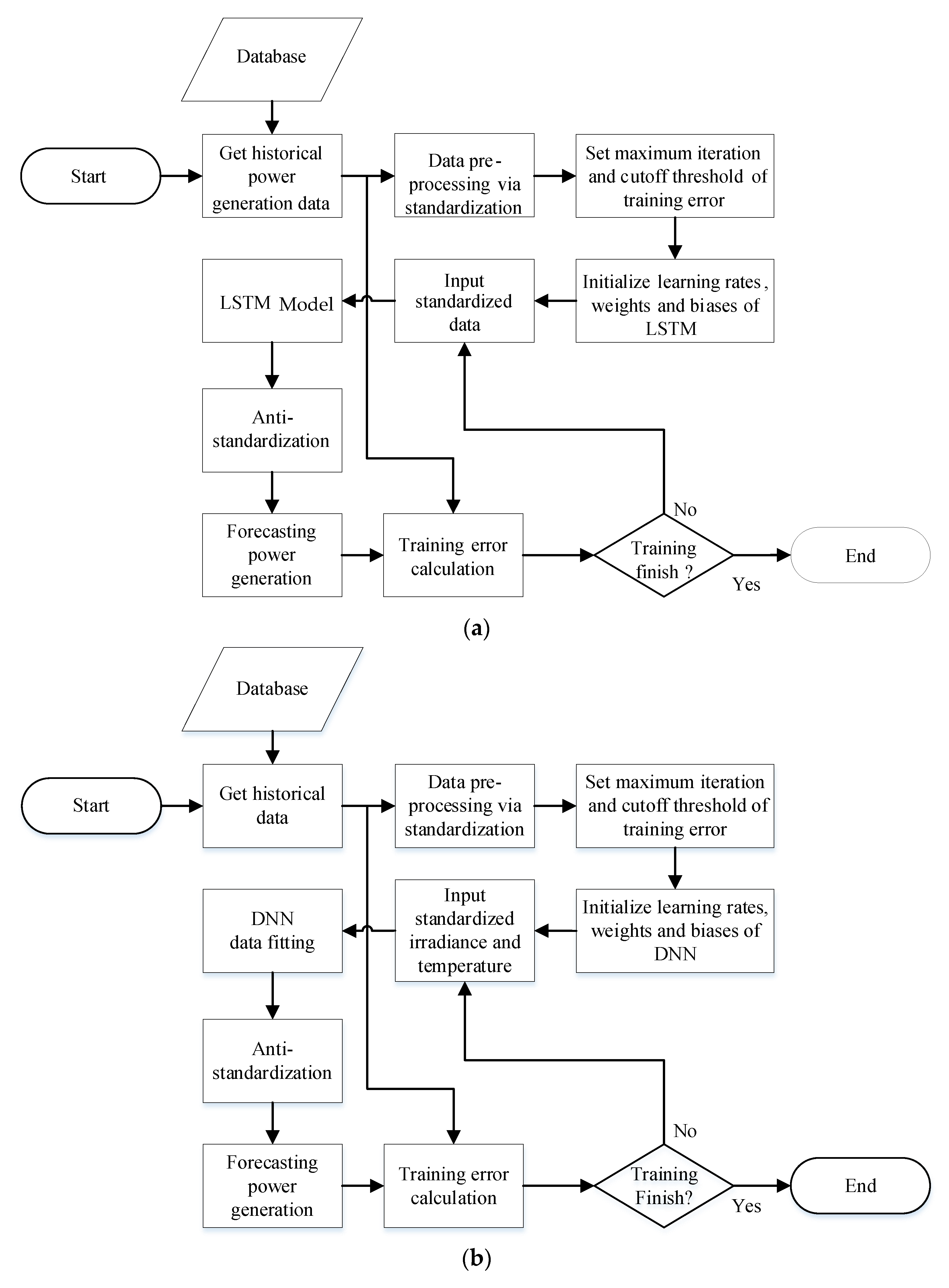
  • Step 1: Obtain historical solar PV power generation data from the database.
  • Step 2: Data preprocessing via the data standardization in (8).
  • Step 3: Set the maximum iteration of the training process and the cutoff threshold of the training error.
  • Step 4: Initialize the learning rates, the weights and the biases of the LSTM in Section 3.
  • Step 5: Input standardized solar PV power generation data into the LSTM.
  • Step 6: Obtain the forecasting power generation via the data anti-standardization in (9) from the LSTM output.
  • Step 7: Calculate the training error between the actual power generation and the forecasting one, and then use training errors to adjust the parameters in the LSTM.
  • Step 8: Repeat steps 5–7 and check whether the maximum iteration of the training process or the cutoff threshold of the training error is achieved.
  • Step 9: Finish the training process if the terminated condition is satisfied.
Moreover, the detail training process of the DNN data fitting in the proposed model is depicted in Figure 4b and is expressed as follows:
  • Step 1: Obtain historical solar PV power generation, irradiance and temperature data from the database.
  • Step 2: Data preprocessing via the data standardization in (8).
  • Step 3: Set the maximum iteration of the training process and the cutoff threshold of the training error.
  • Step 4: Initialize the learning rates, the weights and the biases of the DNN in (10)–(12).
  • Step 5: Input standardized irradiance and temperature into the DNN.
  • Step 6: Obtain the forecasting power generation via the data anti-standardization in (9) from the DNN output.
  • Step 7: Calculate the training error between the actual power generation and the forecasting one, and then use training errors to adjust the parameters in the DNN.
  • Step 8: Repeat steps 5–7 and check whether the maximum iteration of the training process or the cutoff threshold of the training error is achieved.
  • Step 9: Finish the training process if the terminated condition is satisfied.
In addition, the on-line implementation procedure of the proposed DNN-LSTM model is depicted in Figure 4c and is represented as follows:
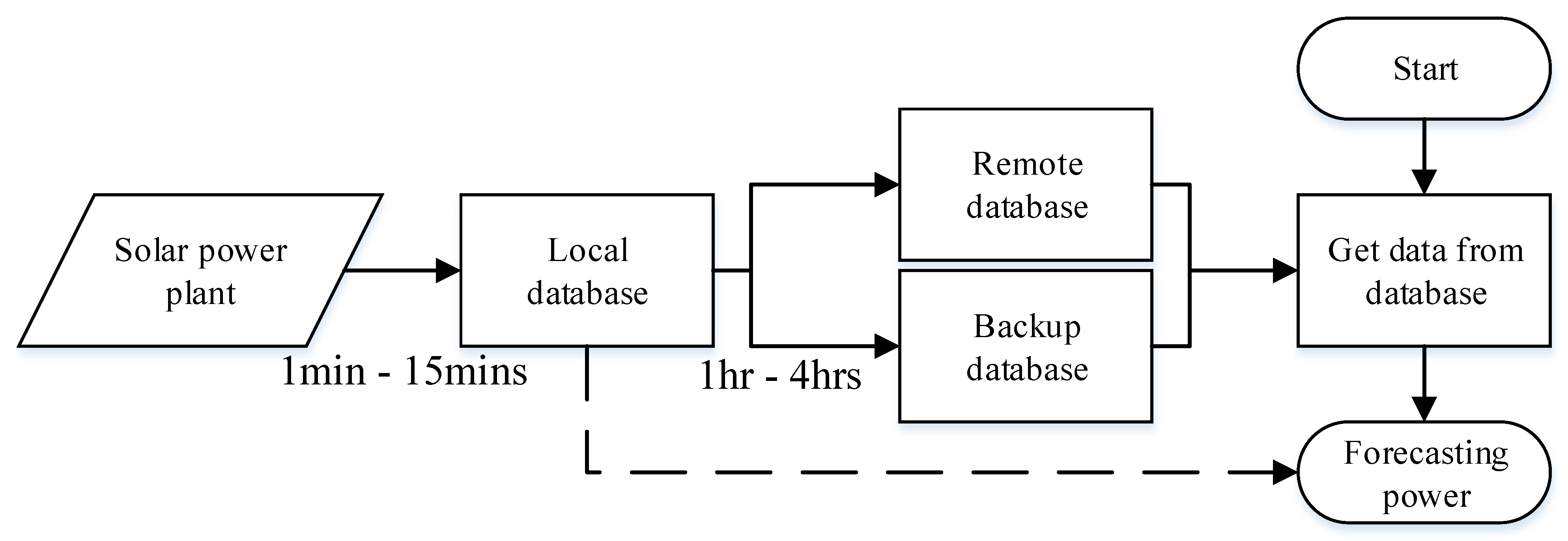
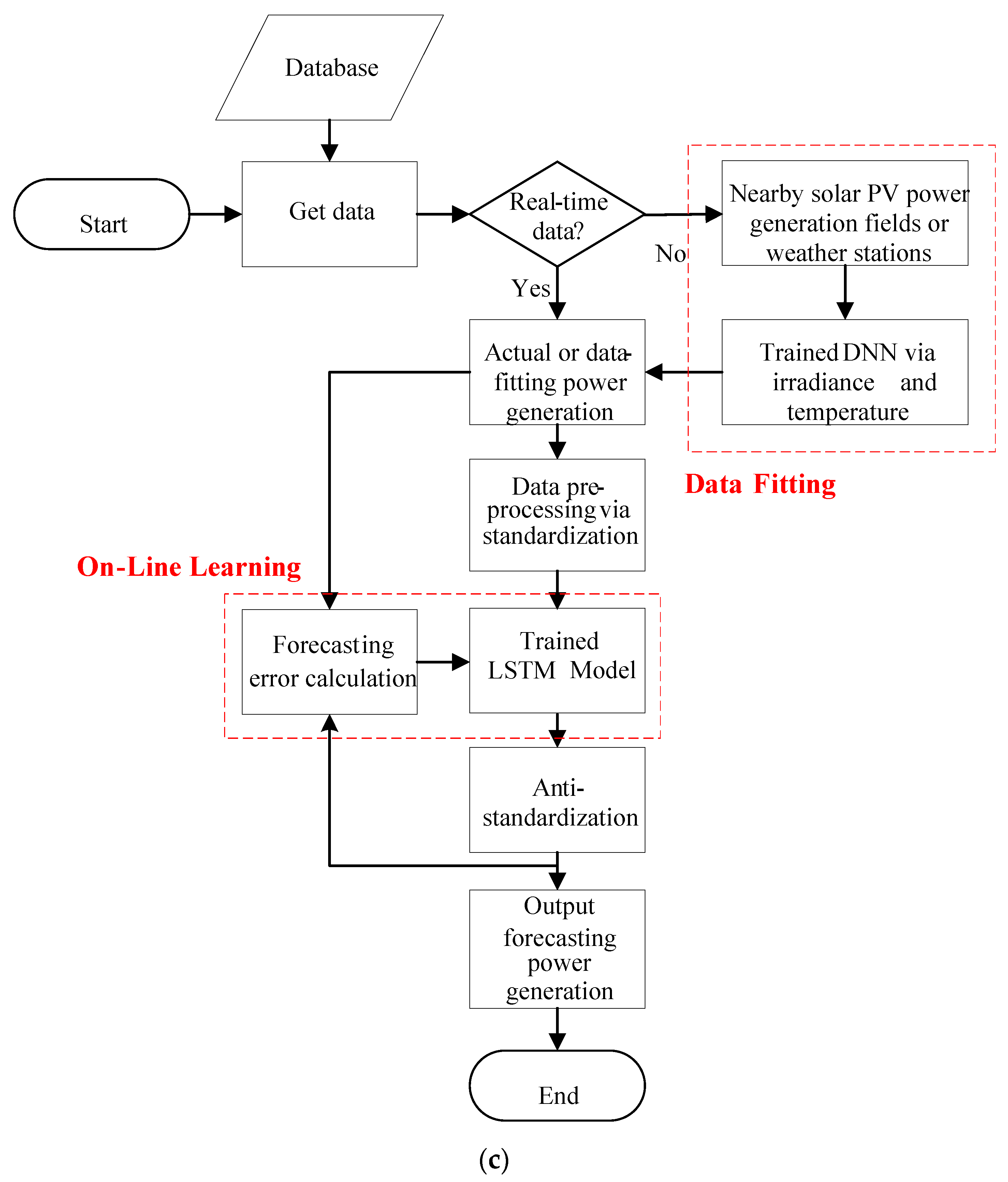
  • Step 1: Obtain data from the database.
  • Step 2: Judge whether the data are real-time solar PV power generation information or not.
  • Step 3: If they are not real-time data, one should obtain the weather information, including irradiance and temperature, from nearby solar PV power generation fields or weather stations, and implement the trained DNN data fitting via steps 5 and 6.
  • Step 4: If they are real-time data, it goes to step 7.
  • Step 5: Input standardized irradiance and temperature into the trained DNN.
  • Step 6: Obtain the data-fitting solar PV power generation via the data anti-standardization in (9) from the trained DNN output.
  • Step 7: Input standardized actual or data-fitting power generation data into the trained LSTM.
  • Step 8: Obtain the forecasting power generation via the data anti-standardization in (9) from the trained LSTM output.
  • Step 9: Calculate the forecasting error between the actual power generation and the forecasting one, and then use forecasting errors to adjust the parameters in the trained LSTM for on-line learning.
  • Step 10: Repeat the above steps until the on-line forecasting programing is finished.

4.5. Performance Evaluation Index

The performance evaluation index is used for the accuracy of a forecasting model and the comparison between different forecasting models. The root-mean-square error (RMSE) is mainly used to measure the deviation between the predicted value and the actual value. It is very sensitive to very large or very small values in a set of data. The RMSE can effectively reflect this forecasting model accuracy. Moreover, the mean absolute error (MAE) is the average of the absolute value of the deviations of all predicted values from the actual values. The MAE will not have the cancelation of positive and negative error values because the difference is absolute. Thus, the MAE can better reflect the actual situation of the forecasting error. In this study, the following three performance evaluation indexes, including the normalized RMSE (nRMSE), the normalized MAE (nMAE), and the accuracy, are adopted:
nRMSE = 1 P c 1 N i = 1 N ( P ^ i P i ) 2
nMAE = 1 N × P c i = 1 N | P ^ i P i |
Accuracy = ( 1 nMAE ) × 100 %
where P i and P ^ i are the actual and forecasting powers of a solar PV power generation system, respectively; P c is the installation capacity of the corresponding solar PV power generation system; and N is the total data numbers.

5. Experimental Results

Experimental setup and performance verification of the proposed intelligent solar photovoltaic (PV) power generation forecasting mechanism combined with weather information under the absence of real-time power generation data are given in this section. In the proposed framework, a deep neural network (DNN) via weather information can be used to compensate the data missing of real-time power generation. Then, the fitting data or the real-time data are sent to a long short-term memory neural network (LSTM) for forecasting the amount of solar PV power generation. In order to verify the effectiveness of the proposed DNN plus LSTM (DNN-LSTM) scheme, six actual solar PV power generation cases labeled in Figure 5 are considered. As for the sites divided by regions in Figure 5, they can be divided into the north, mid-west, south and east in Taiwan. If they are distinguished by the installation capacity of solar PV power generation cases, the smallest case is the solar power plant A of 48 kW, and the largest case is the solar power plant D of 481.2 kW. All forecasting models are implemented by the software of MATLAB 2019 and executed on a desktop with Intel i7-2600 CPU, 16 G RAM, and GPU 2060. The data record periods during one week for six actual solar power plants in Taiwan are summarized in Table 4. Due to the data completeness available from the database, different weekly time periods for the dataset in six actual plants are used in this study.

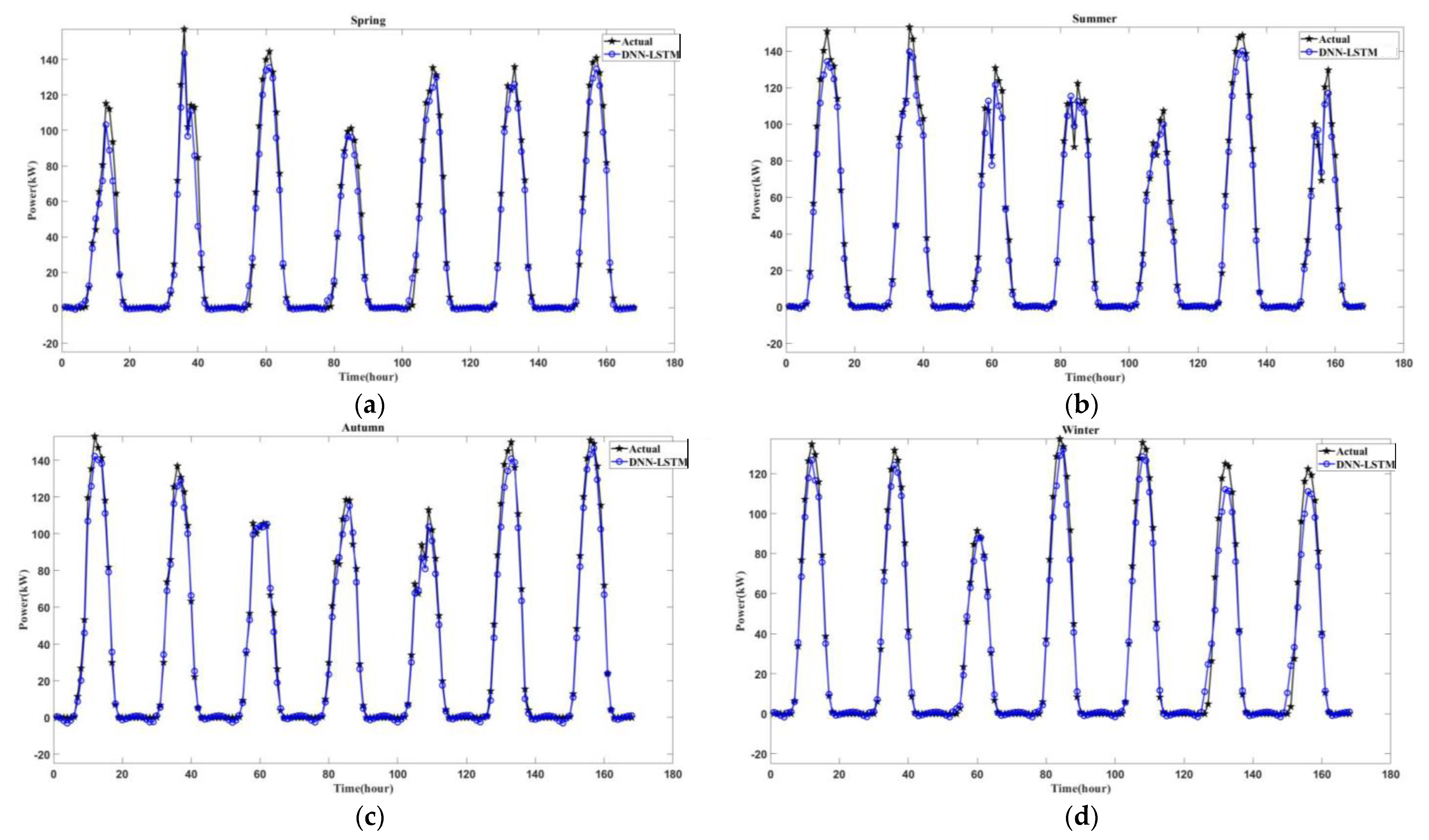
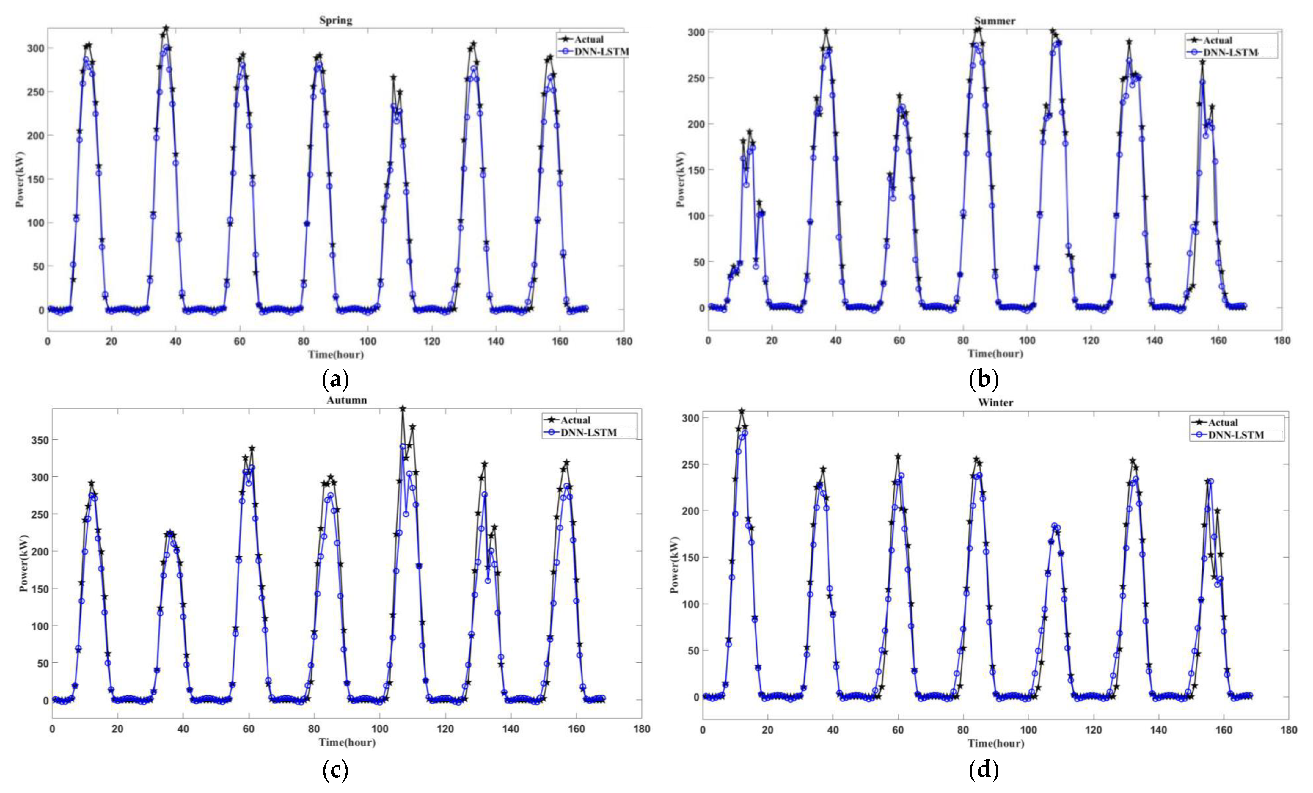
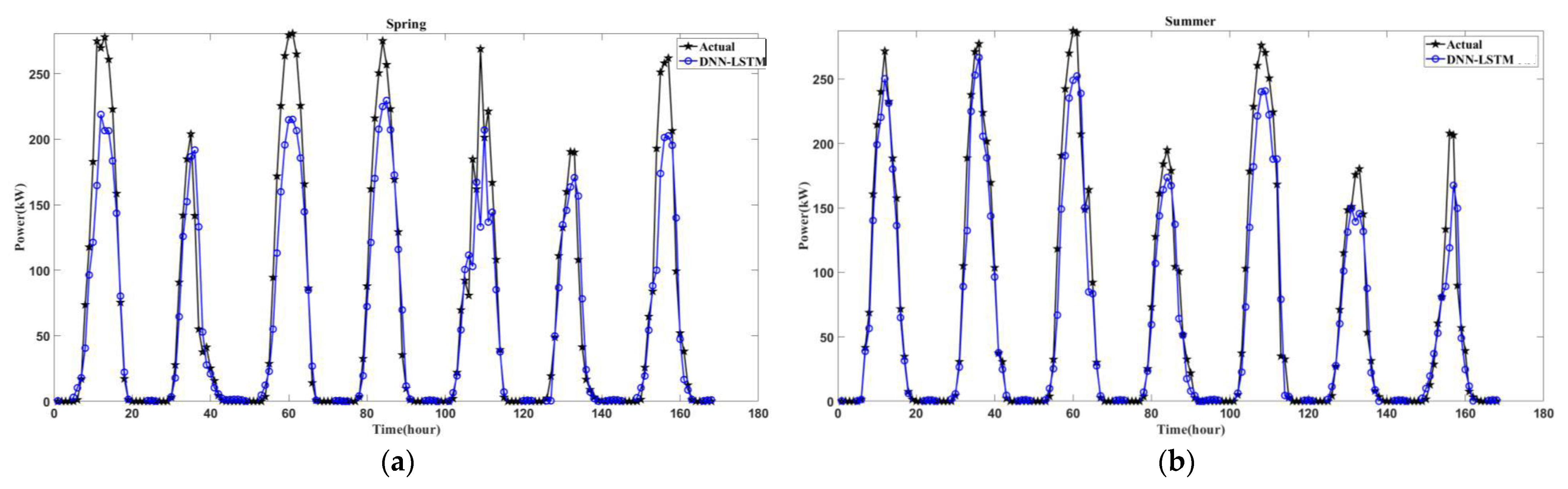
5.1. Solar PV Power Generation Forecasting

In the experiments, the hour forecasting of solar PV power generation will be conducted during one week for each of the four seasons of spring, summer, autumn and winter in these six cases. Moreover, four conventional forecasting strategies, including the long short-term memory neural network (LSTM) in [39], the DNN in [43], the support vector machine (SVM) in [44], and the back-propagation neural network (BPNN) in [45], are also examined to verify the superiority of the proposed DNN-LSTM scheme. In the SVM, a linear kernel function is adopted. All the DNN, BPNN, LSTM, and DNN-LSTM have the full-connection network structure with four layers, and the maximum iteration of the training process is set as 200. In addition, the cutoff threshold of the training error is set as 0.02, and the initial learning rate is set as 0.005. When the forecasting error gradually converges, the learning rate is reduced to 0.001 as 125 iterations to avoid the overfitting problem. The input training data for the LSTM in the proposed model are hourly solar PV power generation data during one year, i.e., the amount of total training data is 8760. Furthermore, the input training data for the DNN data fitting in the proposed model are hourly irradiance and temperature data during one year, i.e., the amount of total training data is 8760 × 2. Except for the proposed scheme with the compensation of the DNN data fitting for real-time solar PV power generation, the other four comparative methods in [39,43,44,45] forecast solar PV power generation via historical data at the next four hours in these experiments.

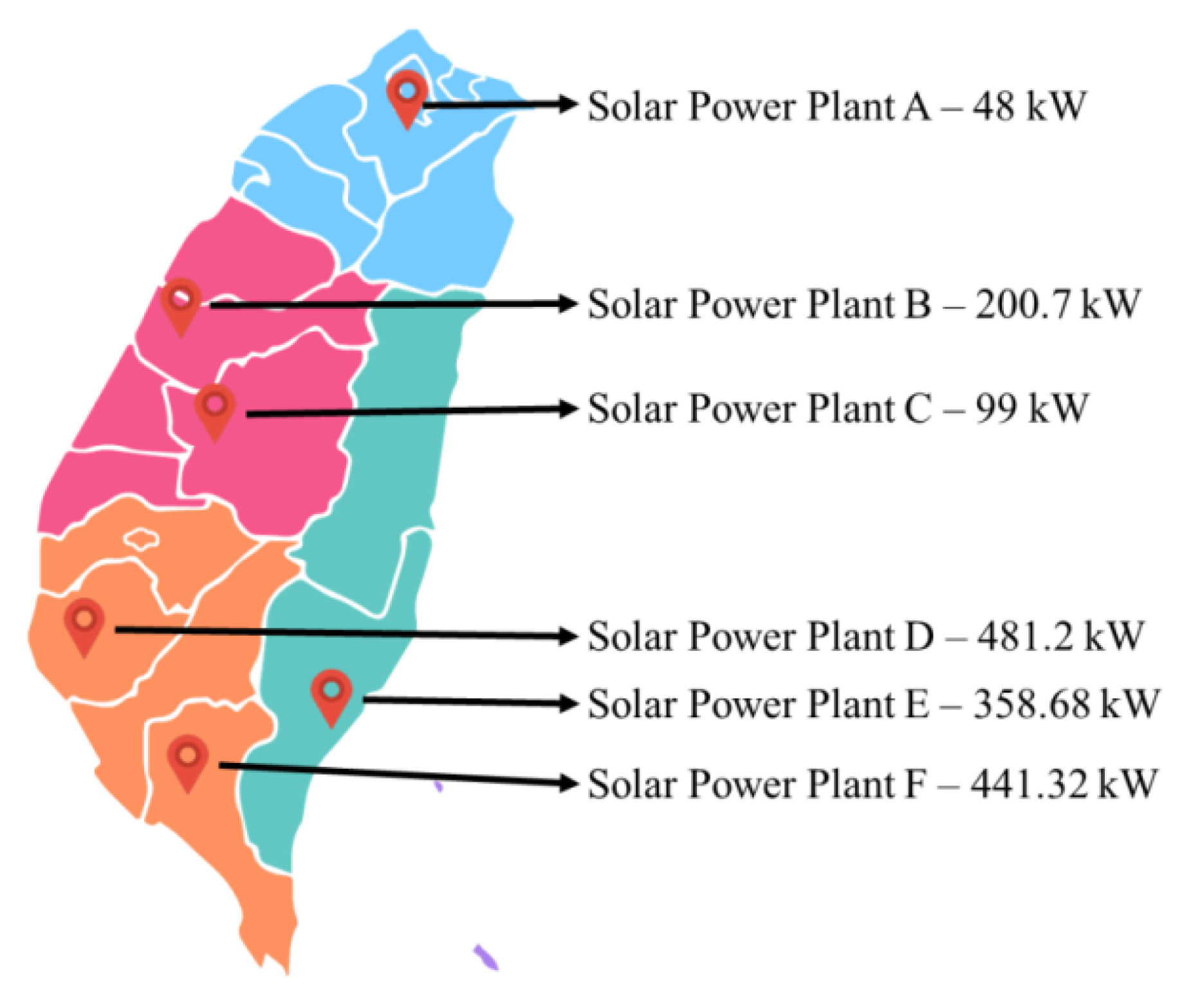
5.1.1. Solar Power Plant A

As for the solar power plant A, the installation capacity is 48 kW, and the site location is in north Taiwan. The hourly power generation forecasting results by the proposed DNN-LSTM scheme during one week for the solar power plant A are depicted in Figure 6, where forecasting results at four seasons of spring, summer, autumn and winter are given in Figure 6a–d, respectively. As can be seen from Figure 6, the overall forecasting of the proposed DNN-LSTM scheme is closer to the actual power generation curve. The comparisons of the normalized root-mean-square error (nRMSE) in (13), the normalized mean absolute error (nMAE) in (14), and the accuracy in (15) of five forecasting models, including the LSTM in [39], the DNN in [43], the SVM in [44], the BPNN in [45], and the proposed DNN-LSTM, for the power plant A are summarized in Table 5. As can be seen from Table 5, the performance of the DNN for solar PV power generation forecasting is the worst one compared to other methods due to the scheme in [43] without parameter optimization in this test. The BPNN and the SVM have good forecasting results for part of the time. Factors, such as severe weather changes, may cause the forecasting effect of the BPNN to deteriorate. For the LSTM, due to the lack of real-time data, if the solar PV power generation of the week is generally stable and there is no special change, the forecasting effect of solar PV power generation can work well. When relative weather changes and other factors lead to large changes in solar PV power generation, its forecasting effect will be relatively poor. As can be seen from Table 5, the proposed DNN-LSTM scheme has an average value of 1.63% of normalized mean absolute error (nMAE), an average value of 2.7% of normalized root mean square error (nRMSE), and an average accuracy of 98.37%. Moreover, the standard deviations of nMAE, nRMSE, and accuracy are 0.67, 1.39, and 0.67%, respectively.

5.1.2. Solar Power Plant B

As for the solar power plant B, the installation capacity is 200.7 kW, and the site location is the mid-west of Taiwan. The hourly power generation forecasting results by the proposed DNN-LSTM scheme during one week for the solar power plant B are depicted in Figure 7, where forecasting results at four seasons of spring, summer, autumn and winter are given in Figure 7a–d, respectively. As can be seen from Figure 7, the overall forecasting of the proposed DNN-LSTM scheme can follow the actual power generation curve. The comparisons of performance indicators of five forecasting models for the power plant B are summarized in Table 6. As can be seen from Table 6, the performance of the DNN for solar PV power generation forecasting is the worst one compared with other methods due to the scheme in [43] without parameter optimization in this test. Further, the BPNN forecasting in this case cannot find the forecasting trend, and there is sudden extreme forecasting value due to the possible occurrence of local minimum weight updating. For the LSTM alone, the forecasting effect is unstable due to the lack of real-time data. As can be seen from Table 6, the proposed DNN-LSTM scheme has an average value of 1.84% of nMAE, an average value of 2.94% of nRMSE, and an average accuracy of 98.16%.

5.1.3. Solar Power Plant C

As for the solar power plant C, the installation capacity is 99 kW, and the site location is the mid-west of Taiwan. The hourly power generation forecasting results by the proposed DNN-LSTM scheme during one week for the solar power plant C are depicted in Figure 8, where forecasting results at four seasons of spring, summer, autumn and winter are given in Figure 8a–d, respectively. As can be seen from Figure 8, the overall forecasting of the proposed DNN-LSTM scheme also can follow the actual power generation curve. The comparisons of performance indicators of five forecast models for the power plant C are summarized in Table 7. Compared with the DNN in [43], the SVM in [44], and the BPNN in [45], the forecasting effect of the LSTM alone in this experiment is the worst. The BPNN, the DNN, and the SVM have poor overall forecasting effect in this experiment due to the lack of real-time solar PV power generation data. As can be seen from Table 7, the proposed DNN-LSTM scheme has an average value of 2.64% of nMAE, an average value of 4.4% of nRMSE, and an average accuracy of 97.36%.

5.1.4. Solar Power Plant D

As for the solar power plant D, the installation capacity is 481.2 kW, and the site location is in south Taiwan. The hourly power generation forecasting results by the proposed DNN-LSTM scheme during one week for the solar power plant D are depicted in Figure 9, where forecasting results at four seasons of spring, summer, autumn and winter are given in Figure 9a–d, respectively. As can be seen from Figure 9, the overall forecasting of the proposed DNN-LSTM scheme also can follow the actual power generation curve. The comparisons of performance indicators of five forecasting models for the power plant D are summarized in Table 8. The LSTM alone has a good effect in the forecasting of some time periods, but the forecasting effect will be worse if the weather changes too sharply. The BPNN, the DNN and the SVM still have poor overall forecasting effect without real-time solar PV power generation data. As can be seen from Table 8, the proposed DNN-LSTM scheme has an average value of 2.54% of nMAE, an average value of 3.46% of nRMSE, and an average accuracy of 97.94%.

5.1.5. Solar Power Plant E

As for the solar power plant E, the installation capacity is 358.68 kW, and the site location is in east Taiwan. The hourly power generation forecasting results by the proposed DNN-LSTM scheme during one week for the solar power plant E are depicted in Figure 10, where forecasting results at four seasons of spring, summer, autumn and winter are given in Figure 10a–d, respectively. As can be seen from Figure 10, the overall forecasting of the proposed DNN-LSTM scheme also can follow the actual power generation curve. The comparisons of performance indicators of five forecasting models for the power plant E are summarized in Table 9. The LSTM and the SVM are effective in forecasting a specific number of days. If the weather condition changes too sharply, the forecasting effect will be worse. The overall forecasting performance of the BPNN and the DNN in this experiment are worse than the LSTM, the SVM and the proposed DNN-LSTM. As can be seen from Table 9, the proposed DNN-LSTM scheme has an average value of 2.87% of nMAE, an average value of 5.1% of nRMSE, and an average accuracy of 97.13%.

5.1.6. Solar Power Plant F

As for the solar power plant F, the installation capacity is 441.32 kW, and the site location is in the south of Taiwan. The hourly power generation forecasting results by the proposed DNN-LSTM scheme during one week for the solar power plant F are depicted in Figure 11, where forecasting results at four seasons of spring, summer, autumn and winter are given in Figure 11a–d, respectively. As can be seen from Figure 11, the overall forecasting of the proposed DNN-LSTM scheme also can follow the actual power generation curve. The comparisons of performance indicators of five forecast models for the power plant F are summarized in Table 10. Except for instantaneous large power generation change, the LSTM alone can work well in this experiment. The overall forecasting performance of the BPNN and the DNN in this experiment are still worse than the LSTM, the SVM and the proposed DNN-LSTM. As can be seen from Table 10, the proposed DNN-LSTM scheme has an average value of 2.26% of nMAE, an average value of 3.1% of nRMSE, and an average accuracy of 98.29%.

5.2. Discussion

The depth analyses of the experimental results in Section 5.1 are given here. Average performance indicators of five forecasting models, including the LSTM in [39], the DNN in [43], the SVM in [44], the BPNN in [45], and the proposed DNN-LSTM, for six actual solar power plants in Taiwan are summarized in Table 11. As can be seen from Table 11, the average values of nMAE, nRMSE, and accuracy of the proposed DNN-LSTM-NN model are 2.03%, 3.62%, and 97.88%, respectively. By comparing the performance of the LSTM in [39], the DNN in [43], the SVM in [44], and the BPNN in [40], the maximum improvement rates of nMAE, nRMSE, and accuracy by the proposed DNN-LSTM model can achieve 81.41%, 77.51%, and 9.88%, respectively. Except for the proposed scheme with the compensation of the DNN data fitting for real-time solar PV power generation, the other four comparative methods in [39,43,44,45] should forecast solar PV power generation via historical data at the next four hours such that their forecasting accuracies are lower than the one of the proposed DNN-LSTM framework. Even for the LSTM-NN alone with memory cells, its average forecasting accuracy is still slightly lower than the proposed DNN-LSTM scheme. It can conclude that the compensation of the DNN data fitting is helpful to enhance the forecasting accuracy of the LSTM model.
Due to various data record times in Table 4, the climatic conditions and the corresponding PV power generation amount are also very different. Moreover, six actual solar PV power stations have different power installation capacities, and are located in various geographical positions. Thus, the maximum performance of the models in each solar power plant will vary with seasons, as shown in Table 5, Table 6, Table 7, Table 8, Table 9 and Table 10. In addition, the smallest PV power station is the plant A, and its PV power change is also the smallest. Because the most frequent severe weather and typhoons occur in the eastern part of Taiwan, the PV power change of the plant E will be the largest. As can be seen from Table 11, the best forecasting result of the proposed model occurs at the plant A, and the worse at the plant E.
In order to show the superiority of the proposed approach compared to statistical methods, a linear regression (LR) model and an auto-regressive integrated moving average (ARIMA) model are further constructed and tested via the same datasets from six solar power plants in Section 5.1. The performance indexes of LR and ARIMA forecasting models are summarized in Table 12. The average accuracy of the LR forecasting model in Table 12 is 83.65% because the solar PV power generation data are rarely linearly separable. Although the ARIMA model can be quite adept when it comes to modeling the overall trend of a series along with seasonal patterns, the outliers of solar PV power generation caused by weather conditions will limit its forecasting accuracy. Thus, the average accuracy of the ARIMA forecasting model in Table 12 is 92.18%. By comparing the records in Table 12 with Table 11, it is obvious that the forecasting performance of artificial intelligence (AI)-based models is superior to that of stochastic-based models. Compared to the performance of the LR model and the ARIMA model, the maximum average improvement rates of nMAE, nRMSE, and accuracy by the proposed DNN-LSTM model can achieve 87.58%, 81.62%, and 17.01%, respectively.
The execution times required for five forecasting models, including the LSTM in [39], the DNN in [43], the SVM in [44], the BPNN in [45], and the proposed DNN-LSTM, to predict a single datum and the corresponding training runtimes are summarized in Table 13. As can be seen from Table 13, it can be found that the proposed DNN-LSTM model requires a longer execution time. Fortunately, the overall forecasting trend and precise indicators by the proposed DNN-LSTM model are relatively high in comparisons with the other four models. In terms of hourly solar PV power generation forecasting, the execution time for a single power generation forecasting by the proposed DNN-LSTM model is only 0.12 s to be smaller than the sunlight change rate and the minute-level sampling time. The execution time of the proposed model can be faster than the data sampling, which paves the way for realistic applications. Thanks to the powerful computing speed of the current processors or industrial computers, it is not a problem in practical applications, although the proposed DNN-LSTM model with better forecasting performance takes longer training runtimes than other methods.

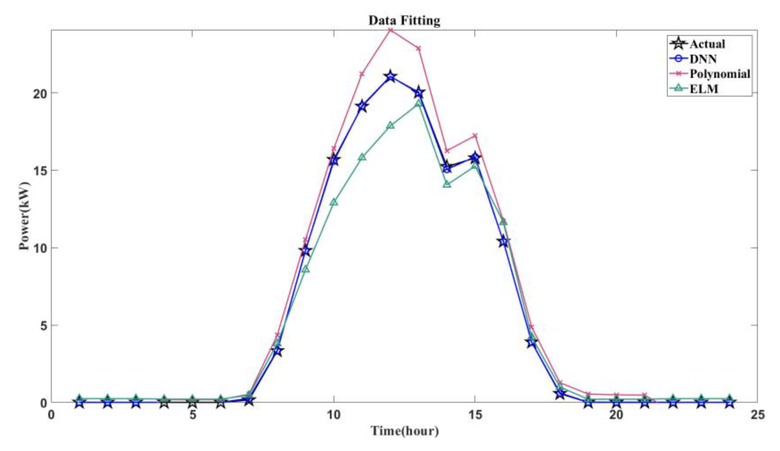
5.3. Data Fitting Performance with Irradiance and Temperature

In order to show the superiority of the DNN for compensating the missing data with weather information, the data-fitting performance of the polynomial regression (PR) in [46] and the extreme learning machine (ELM) in [47] are also examined here. The data-fitting results of the DNN, the PR in [46] and the ELM in [47] are depicted in Figure 12, and the corresponding comparative indexes are summarized in Table 14. As can be seen from Figure 12, the data-fitting power generation by the DNN, and the actual power generation almost completely overlap. Moreover, the data-fitting effect of the PR in [46] and the ELM in [47] can follow some power generation trends. In Table 14, it can be clearly seen that the data-fitting effect of the DNN is better than the performance of the PR in [46] and the ELM in [47].

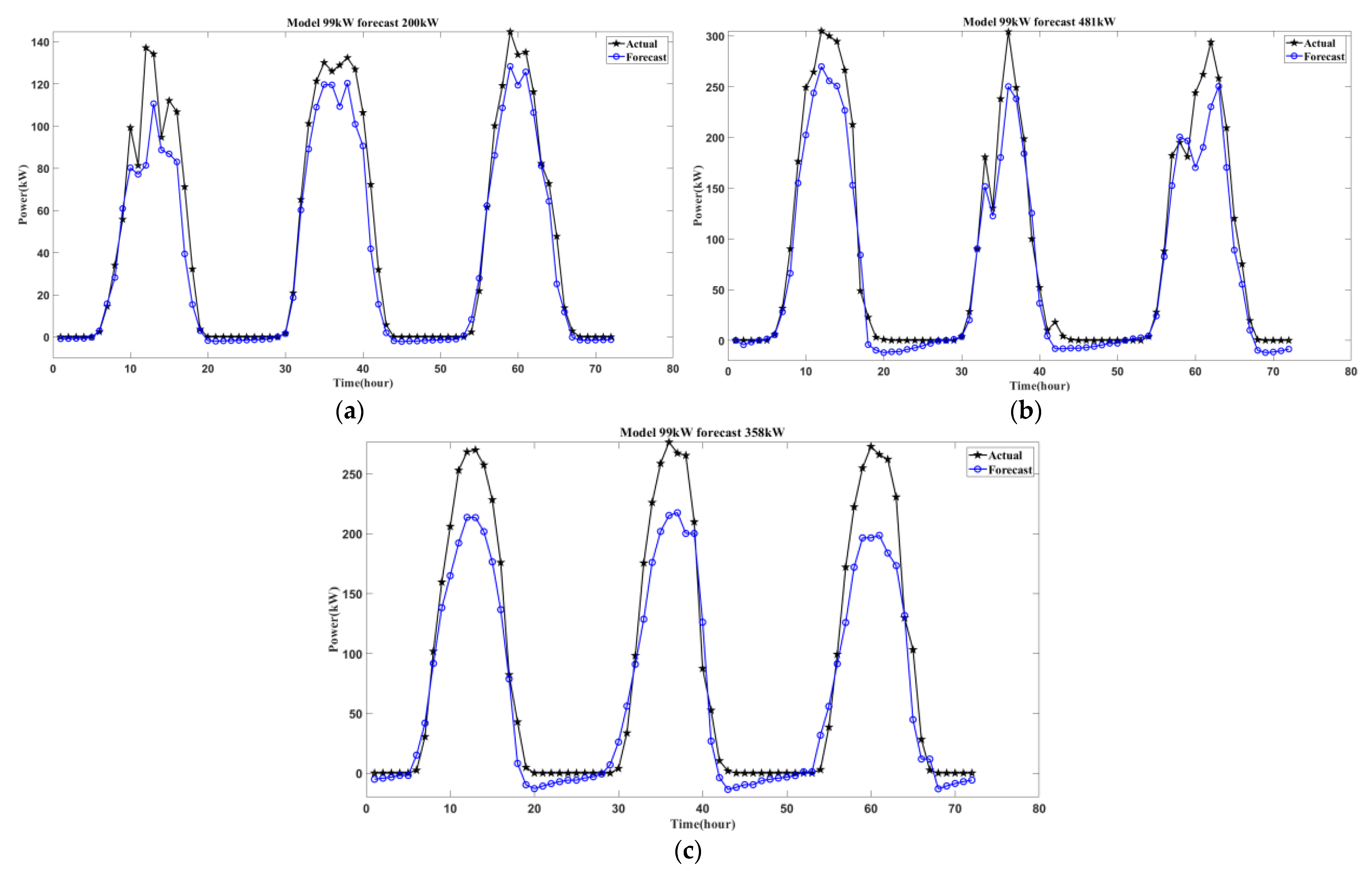
5.4. Model Universal Applicability Verification

In order to test the model universal applicability, the data of the solar power plant C with the installed capacity of 99 kW are used to train the proposed DNN-LSTM model. Then, the data of solar power plants B (200.7 kW), D (481.2 kW), and E (358.68 kW) are adopted for verifying the trained model. The forecasting result via the data of the solar power plant B is depicted in Figure 13a; the one via the data of the solar power plant D is depicted in Figure 13b; and the one via the data of the solar power plant E is depicted in Figure 13c. Due to the uneven changes in solar PV power generation, the proposed DNN-LSTM model can effectively forecast the trend of solar PV power generation, although the maximum peak cannot be effectively predicted in Figure 13. The discrepancies between the actual curves and the forecast ones are different in various plants because the model, which was trained by the data from the solar power plant C (99 kW), is tested by the data of solar power plants B (200.7 kW), D (481.2 kW), and E (358.68 kW). The larger the PV installation capacity difference, the larger the forecasting peak error. In the future research, it could be improved by forecasting the power generation change rate to replace the power generation amount in this study.

5.5. On-Line Learning Ability Verification

In order to verify the performance of the proposed model with on-line learning ability, the power generation data of solar power plant E on 18 June 2021 are repeated during six cycles to test the forecasting performance, as shown in Figure 14a, and the corresponding nMAE and nRMSE values are depicted in Figure 14b. Although the forecasting power generation cannot track the peak value of the actual one during the first cycle, the proposed model can adjust its network parameters according to the forecasting error. As can be seen from Figure 14, it is obvious that the forecasting power generation can track the actual one after two cycles, and the values of nMAE and nRMSE perform stably after the third cycle.

6. Conclusions

This study has successfully designed an intelligent solar photovoltaic (PV) power generation forecasting mechanism combined with weather information under the absence of real-time power generation data. Moreover, it also has been successfully applied for the power generation forecasting of various solar PV areas in Taiwan. Aiming at the problem that the delayed data transmission caused by cost reduction consideration, communication traffic restrictions, or data missing may lead to a decrease in the accuracy of solar PV power generation forecasting due to the inability to obtain real-time data, this study has adopted the irradiance and temperature data provided by nearby solar PV power generation fields or weather stations as an auxiliary to use a deep neural network (DNN) to compensate the data missing of real-time power generation. As for the data-fitting performance of the DNN, the normalized mean absolute error (nMAE) is 0.44%, and the normalized root-mean-square error (nRMSE) is 0.94%. From the data-fitting performance of the DNN in comparisons with the polynomial regression (PR) in [46] and the extreme learning machine (ELM) in [47], the improvement rates of nMAE and nRMSE compared to the PR are 85.67% and 81.92%, respectively; the improvement rates of nMAE and nRMSE compared to the ELM are 79.62% and 76.5%, respectively.
The DNN combined with the long short-term memory neural network (LSTM) to form the proposed DNN-LSTM model can achieve a high hour-forecasting accuracy of over 97% in six solar PV power stations for testing a week in every season or all days in a season. The significant advantages of this study are summarized as follows: (1) the Pearson correlation coefficient analysis is used to reduce related factor requirement for the data fitting of solar PV power generation in comparison with [37]. (2) Only the selection of irradiance and temperature as the input data of the DNN is helpful to alleviate the computing burden, and the corresponding data-fitting performance is superior to the ones of the PR in [46] and the ELM in [47]. (3) Only the power generation data are required as the input for the LSTM in the proposed strategy, and the forecasting accuracy of the proposed DNN-LSTM model is better than the ones of the LSTM in [39], the DNN in [43], the support vector machine (SVM) in [44], and the back-propagation neural network (BPNN) in [45]. (4) The proposed DNN-LSTM model with on-line learning mechanism is helpful to adjust the trained model to adapt different solar power plants or environmental conditions.
From the perspective of model versatility, it is verified whether the model can be universally used in various solar PV power generation cases. The experimental results show that the model has a high versatility. Therefore, it can be used for different solar PV power generation cases. The previously established model directly performs model prediction, which can effectively reduce the time required for retraining and establishing the model. Although the proposed model with only the input information of power generation can predict the trend of solar PV power generation, it cannot fully predict the peak value of actual power generation. Two striking suggestions can be made for future studies. The first one is to add more feature factors (e.g., solar zenith angle, sky type, etc.) for improving the forecasting accuracy. The other one is the replacement of power generation amount forecasting by the change rate prediction, and it may be workable for solar power plants with different installed capacities.

Author Contributions

Conceptualization, P.-X.L.; methodology, P.-X.L. and R.-J.W.; software, P.-X.L.; formal analysis, P.-X.L.; writing—original draft preparation, R.-J.W.; writing—review and editing, R.-J.W.; project administration, R.-J.W.; funding acquisition, R.-J.W. All authors have read and agreed to the published version of the manuscript.

Funding

This research was funded in part by Ministry of Science and Technology of Taiwan grant number 108-2221-E-011-080-MY3.

Conflicts of Interest

The authors declare no conflict of interest.

References

  1. IEA. Global Energy Review 2020. The Impacts of the COVID-19 Crisis on Global Energy Demand and CO2 Emission. International Energy Agency. 2020. Available online: https://www.iea.org/reports/global-energy-review-2020 (accessed on 1 May 2022).
  2. Cirés, E.; Marcos, J.; de la Parra, I.; García, M.; Marroyo, L. The potential of forecasting in reducing the LCOE in PV plants under ramp-rate restrictions. Energy 2019, 188, 116053. [Google Scholar]
  3. IEA. Renewable Energy Market Update-May 2022. International Energy Agency. 2022. Available online: https://www.iea.org/reports/renewable-energy-market-update-may-2022 (accessed on 1 May 2022).
  4. Golubchik, L.; Khuller, S.; Mukherjee, K.; Yao, Y. To send or not to send: Reducing the cost of data transmission. In Proceedings of the 2013 Proceedings IEEE INFOCOM, Turin, Italy, 14–19 April 2013; pp. 2472–2478. [Google Scholar]
  5. Porter, K.; Fink, S.; Buckley, M.; Rogers, J.; Hodge, B.M. Review of Variable Generation Integration Charges; Technical Report NREL/TP-5500-57583; National Renewable Energy Laboratory: Golden, CO, USA, 2013.
  6. Lew, D.; Piwko, N.; Miller, D.; Jordan, G.; Clark, K.; Freeman, L. NREL: How do High Levels of Wind and Solar Impact the Grid? The Western Wind and Solar Integration Study; Technical Report NREL/TP-5500-50057; National Renewable Energy Laboratory: Golden, CO, USA, 2010.
  7. Shaker, H.; Manfre, D.; Zareipour, H. Forecasting the aggregated output of a large fleet of small behind-the-meter solar photovoltaic sites. Renew. Energy 2020, 147, 1861–1869. [Google Scholar]
  8. Ketterer, J.C. The impact of wind power generation on the electricity price in Germany. Energy Econ. 2014, 44, 270–280. [Google Scholar]
  9. Vos, K.D. Negative wholesale electricity prices in the German, French and Belgian day-ahead, intra-day and real-time markets. Electr. J. 2015, 28, 36–50. [Google Scholar] [CrossRef]
  10. Elliott, E. Green Power Curtailment in China. Renewable: Option and Review. 2019. Available online: https://physicsworld.com/a/green-power-curtailment-in-china/ (accessed on 1 May 2022).
  11. Tang, N.; Zhang, Y.; Niu, Y.; Du, X. Solar energy curtailment in China: Status quo, reasons and solutions. Renew. Sustain. Energy Rev. 2018, 97, 509–528. [Google Scholar] [CrossRef]
  12. Li, C.; Shi, H.; Cao, Y.; Wang, J.; Kuang, Y.; Tan, Y.; Wei, J. Comprehensive review of renewable energy curtailment and avoidance: A specific example in China. Renew. Sustain. Energy Rev. 2015, 41, 1067–1079. [Google Scholar]
  13. Chou, K.L. Constructing a power system with high renewable energy ratios in Taiwan: The key issues of long-term developmental pathways and energy storage strategies to fulfill net-zero emissions. Sustain. Ind. Dev. Newsl. 2021, 22, 7–8. [Google Scholar]
  14. Yang, D.; Dong, Z. Operational photovoltaics power forecasting using seasonal time series ensemble. Sol. Energy 2018, 166, 529–541. [Google Scholar] [CrossRef]
  15. Wang, G.; Su, Y.; Shu, L. One-day-ahead daily power forecasting of photovoltaic systems based on partial functional linear regression models. Renew. Energy 2016, 96, 469–478. [Google Scholar] [CrossRef] [Green Version]
  16. Kang, M.; Sohn, J.; Park, J.; Lee, S.; Yoon, Y. Development of algorithm for day ahead PV generation forecasting using data mining method. In Proceedings of the IEEE 54th International Midwest Symposium on Circuits and Systems (MWSCAS), Seoul, Korea, 7–10 August 2011; pp. 1–4. [Google Scholar]
  17. Kashyap, Y.; Bansal, A.; Sao, A.K. Solar radiation forecasting with multiple parameters neural networks. Renew. Sustain. Energy Rev. 2015, 49, 825–835. [Google Scholar]
  18. Kushwaha, V.; Pindoriya, N.M. Very short-term solar PV generation forecast using SARIMA model: A case study. In Proceedings of the 7th International Conference on Power Systems (ICPS), Pune, India, 21–23 December 2017; pp. 430–435. [Google Scholar]
  19. Pierro, M.; Bucci, F.; Felice, M.D.; Maggioni, E.; Moser, D.; Perotto, A.; Spada, F.; Cornaro, C. Multi-model ensemble for day ahead prediction of photovoltaic power generation. Sol. Energy 2016, 134, 132–146. [Google Scholar]
  20. Yang, C.; Thatte, A.A.; Xie, L. Multitime-scale data-driven spatio-temporal forecast of photovoltaic generation. IEEE Trans. Sustain. Energy 2015, 6, 104–112. [Google Scholar] [CrossRef]
  21. Chen, X.; Du, Y.; Wen, H.; Jiang, L.; Xiao, W. Forecasting-based power ramp-rate control strategies for utility-scale PV systems. IEEE Trans. Ind. Electron. 2019, 66, 1862–1871. [Google Scholar] [CrossRef]
  22. Massidda, L.; Marrocu, M. Use of multilinear adaptive regression splines and numerical weather prediction to forecast the power output of a PV plant in Borkum, Germany. Sol. Energy 2017, 146, 141–149. [Google Scholar] [CrossRef]
  23. Reikard, G.; Haupt, S.E.; Jensen, T. Forecasting ground-level irradiance over short horizons: Time series, meteorological, and time-varying parameter models. Renew. Energy 2017, 112, 474–485. [Google Scholar] [CrossRef]
  24. Mellit, A.; Pavan, A.M.; Lughi, V. Short-term forecasting of power production in a large-scale photovoltaic plant. Sol. Energy 2014, 105, 401–413. [Google Scholar] [CrossRef]
  25. Leva, S.; Dolara, A.; Grimaccia, F.; Mussetta, M.; Ogliari, E. Analysis and validation of 24 hours ahead neural network forecasting of photovoltaic output power. Math. Comput. Simul. 2017, 131, 88–100. [Google Scholar] [CrossRef] [Green Version]
  26. Durrani, S.P.; Balluff, S.; Wurzer, L.; Krauter, S. Photovoltaic yield prediction using an irradiance forecast model based on multiple neural networks. J. Mod. Power Syst. Clean Energy 2018, 6, 255–267. [Google Scholar] [CrossRef]
  27. Alfadda, A.; Rahman, S.; Pipattanasomporn, M. Solar irradiance forecast using aerosols measurements: A data driven approach. Sol. Energy 2018, 170, 924–939. [Google Scholar] [CrossRef]
  28. Sun, Y.; Venugopal, V.; Brandt, A.R. Convolutional neural network for short-term solar panel output prediction. In Proceedings of the IEEE 7th World Conference Photovoltaic Energy Conversion (WCPEC) (Joint Conf. 45th IEEE PVSC, 28th PVSEC & 34th EU PVSEC), Waikoloa, HI, USA, 10–15 June 2018; pp. 2357–2361. [Google Scholar]
  29. Yu, Y.; Cao, J.; Wan, X.; Zeng, F.; Xin, J.; Ji, Q. Comparison of short-term solar irradiance forecasting methods when weather conditions are complicated. J. Renew. Sustain. Energy 2018, 10, 053501. [Google Scholar] [CrossRef]
  30. Rahman, A.; Srikumar, V.; Smith, A.D. Predicting electricity consumption for commercial and residential buildings using deep recurrent neural networks. Appl. Energy 2018, 212, 372–385. [Google Scholar] [CrossRef]
  31. Tang, P.J.; Wang, H.L.; Xu, K.S. Multi-objective layer-wise optimization and multi-level probability fusion for image description generation using LSTM. Acta Autom. Sin. 2018, 40, 1237–1249. [Google Scholar]
  32. Yang, L.; Zheng, Y.; Cai, X.; Dai, H.; Mu, D.; Guo, L.; Dai, T. A LSTM based model for personalized context-aware citation recommendation. IEEE Access 2018, 6, 59618–59627. [Google Scholar] [CrossRef]
  33. Zhou, H.; Zhang, Y.; Yang, L.; Liu, Q.; Yan, K.; Du, Y. Short-term photovoltaic power forecasting based on long short term memory neural network and attention mechanism. IEEE Access 2019, 7, 78063–78074. [Google Scholar] [CrossRef]
  34. Yu, Y.; Cao, J.; Zhu, J. An LSTM short-term solar irradiance forecasting under complicated weather conditions. IEEE Access 2019, 7, 145651–145666. [Google Scholar] [CrossRef]
  35. Yang, T.; Li, B.; Xun, Q. LSTM-attention-embedding model-based day-ahead prediction of photovoltaic power output using Bayesian optimization. IEEE Access 2019, 7, 171471–171484. [Google Scholar] [CrossRef]
  36. Hossain, M.S.; Mahmood, H. Short-term photovoltaic power forecasting using an LSTM neural network and synthetic weather forecast. IEEE Access 2020, 8, 172524–172533. [Google Scholar] [CrossRef]
  37. Zhang, Y.; Qin, C.; Srivastava, A.K.; Jin, C.; Sharma, R.K. Data-driven day-ahead PV estimation using autoencoder-LSTM and persistence model. IEEE Trans. Ind. Appl. 2020, 56, 7185–7192. [Google Scholar] [CrossRef]
  38. Liu, C.H.; Gu, J.C.; Yang, M.T. A simplified LSTM neural network for one day-ahead solar power forecasting. IEEE Access 2021, 9, 17174–17195. [Google Scholar] [CrossRef]
  39. Hochreiter, S.; Schmidhuber, J. Long short-term memory. Neural Comput. 1997, 9, 1735–1780. [Google Scholar] [CrossRef]
  40. Pareek, V.; Chaudhury, S. Deep learning-based gas identification and quantification with auto-tuning of hyper-parameters. Soft Comput. 2021, 25, 14155–14170. [Google Scholar] [CrossRef]
  41. Neshat, M.; Nezhad, M.M.; Mirjalili, S.; Piras, G.; Garcia, D.A. Quaternion convolutional long short-term memory neural model with an adaptive decomposition method for wind speed forecasting: North aegean islands case studies. Energy Convers. Manag. 2022, 259, 115590. [Google Scholar] [CrossRef]
  42. Xie, Y.Y.; Li, C.S.; Tang, G.; Liu, F.J. A novel deep interval prediction model with adaptive interval construction strategy and automatic hyperparameter tuning for wind speed forecasting. Energy 2021, 216, 119179. [Google Scholar] [CrossRef]
  43. Alzahrani, A.; Shamsi, P.; Dagli, C.; Ferdowsi, M. Solar irradiance forecasting using deep neural networks. Procedia Comput. Sci. 2017, 114, 304–313. [Google Scholar] [CrossRef]
  44. Cortes, C.; Vapnik, V. Support-vector networks. Mach. Learn. 1995, 20, 273–297. [Google Scholar] [CrossRef]
  45. Rumelhart, D.E.; Hinton, G.E.; Williams, R.J. Learning representations by back-propagating errors. Nature 1986, 9, 533–536. [Google Scholar] [CrossRef]
  46. Ostertagová, E. Modelling using polynomial regression. Procedia Eng. 2012, 48, 500–506. [Google Scholar] [CrossRef] [Green Version]
  47. Huang, G.B.; Zhu, Q.Y.; Siew, C.K. Extreme learning machine: Theory and applications. Neurocomputing 2006, 70, 489–501. [Google Scholar] [CrossRef]
Figure 1. Structure of long short-term memory neural network.
Energies 15 03838 g001
Figure 2. Schematic diagram of information acquisition process by solar PV power operator in Taiwan.
Energies 15 03838 g002
Figure 3. Framework of deep neural network.
Energies 15 03838 g003
Figure 4. Solar PV power generation forecasting strategy: (a) training process of LSTM; (b) training process of the DNN data fitting; (c) implementation procedure of proposed DNN-LSTM model.
Energies 15 03838 g004aEnergies 15 03838 g004b
Figure 5. Distribution locations of actual solar PV power generation cases in Taiwan.
Energies 15 03838 g005
Figure 6. Hourly power generation forecasting results by DNN-LSTM during one week for solar power plant A: (a) spring; (b) summer; (c) autumn; (d) winter.
Energies 15 03838 g006aEnergies 15 03838 g006b
Figure 7. Hourly power generation forecasting results by DNN-LSTM during one week for solar power plant B: (a) spring; (b) summer; (c) autumn; (d) winter.
Energies 15 03838 g007
Figure 8. Hourly power generation forecasting results by DNN-LSTM during one week for solar power plant C: (a) spring; (b) summer; (c) autumn; (d) winter.
Energies 15 03838 g008
Figure 9. Hourly power generation forecasting results by DNN- LSTM during one week for solar power plant D: (a) spring; (b) summer; (c) autumn; (d) winter.
Energies 15 03838 g009
Figure 10. Hourly power generation forecasting results by DNN- LSTM during one week for solar power plant E: (a) spring; (b) summer; (c) autumn; (d) winter.
Energies 15 03838 g010aEnergies 15 03838 g010b
Figure 11. Hourly power generation forecasting results by DNN- LSTM during one week for solar power plant F: (a) spring; (b) summer; (c) autumn; (d) winter.
Energies 15 03838 g011
Figure 12. Comparisons of data-fitting performance with irradiance and temperature via DNN, PR and ELM.
Energies 15 03838 g012
Figure 13. Model universality verification via training data of solar power plant C: (a) testing data via solar power plant B; (b) testing data via solar power plant D; (c) testing data via solar power plant E.
Energies 15 03838 g013
Figure 14. Verification of proposed model with on-line learning ability: (a) six consecutive cycles of power generation forecasting; (b) variation in nMAE and nRMSE values.
Energies 15 03838 g014
Table 1. Summary of research background and merits/limitation of previous methods.
ReferencesResearch Background or MeritsLimitations
[14,19]Numerical weather prediction is a method of forecasting that the physical laws of atmospheric behavior are expressed through mathematical equations.It relies heavily on the accuracy of weather forecasting.
[15]Partial functional linear regression can process or predict nonlinear data.There are many characteristic parameters, which are more troublesome to select training parameters.
[16]The method using K-means has a good performance and a fast calculation speed.This algorithm is sensitive to the initial status of clustering, and its performance relies heavily on the accuracy of weather center information.
[17,25]ANN has high accuracy and can process noisy data effectively.This prediction method requires a huge network framework with many coefficients to be adjusted and spends more training time.
[18]SARIMA solves the limitation of ARIMA on seasonality and clarifies the seasonal elements in the simulation data.The processing effect of nonlinear data may be deteriorated.
[20]The prediction effect of spatio-temporal-ARX model is better than persistence model.For different weather conditions, e.g., non-sunny weather, its prediction effect may be degenerate.
[21]A method of DSTR with GBSFS to achieve the objective of solar PV power generation prediction.This method is unsuitable for data with strong noise.
[22]Multi-linear adaptive regression splines method can process or predict nonlinear data.This method needs more input data to improve accuracy, and the input data need to be time-efficient.
[23]It uses ARIMA with DICast and NWP to predict solar PV power generation.Unstable data and inaccurate weather forecasting will lead to a decrease in the forecasting accuracy.
[24]It proposes an AFFNN to judge weather conditions through NWP, and then uses different AFFNNs to predict power generation.This method, which uses three distinct ANN models to be applied to three typical types of day (sunny, partly cloudy and overcast), is more complicated than only one unified model.
[26]The irradiance prediction model via the multi-layer feedforward neural network is used for power generation prediction, which is divided into illuminance, temperature, and energy prediction models.There are lots of input parameters during the training process, and three models to be trained are time-consuming.
[27]It uses the MLP model to predict solar PV power generation in the desert, which can effectively predict power generation on sunny days.Except for sunny day, the effect of the model may be deteriorated for non-sunny days
[28]It uses CNN to predict power generation via sky images and historical power generation data.The training process of CNN is always time-consuming.
[29]RNN is used to predict solar PV power generation.The problem of gradient explosion in RNN should be further avoided.
Table 2. Research comparisons of different forecasting methods in previous research [33,34,35,36,37,38].
ReferencesForecasting MethodInput Feature FactorsWeather DataModel ComplexityRequirement of Real-Time Power Generation Data
[33]LSTM and attention mechanismLess (P,T)NoSimpleYes
[34]LSTM with weather conditionsMore
(P, IR, ST, D PT, T, PW, RH, SZA, WS, WD)
YesHighYes
[35]LSTM-attention-embeddingMore
(P, TI, IR, T, RH, WD)
YesHighYes
[36]LSTM and synthetic weather forecastMore
(P, IR, T, WS, RH, ST)
YesMediumYes
[37]Auto-encoder LSTM and persistence modelMore
(P, T, RH, WS, IR, TI)
YesMediumYes
[38]Simplified LSTMMore
(P, IR, ST, WS)
YesSimpleYes
Table 3. Correlation analyses of solar PV power generation with respect to irradiance and temperature.
Related Factor/R(x,y) ValueIrradianceTemperature
Solar PV power generation0.94320.8561
Table 4. Summary of data record period during one week for six actual solar power plants in Taiwan.
PlantSpringSummerAutumnWinter
AFrom 12 February 2020
to 18 February 2020
From 30 May 2020
to 5 June 2020
From 10 January 2019
to 7 October 2019
From 3 January 2020
to 9 January 2020
BFrom 17 February 2020
to 23 February 2020
From 5 May 2020
to 11 May 2020
From 19 September 2019
to 25 September 2019
From 5 November 2019
to 11 November 2019
CFrom 22 February 2020
to 28 February 2020
From 31 May 2020
to 6 June 2021
From 1 October 2019
to 7 October 2019
From 23 November 2019
to 29 November 2019
DFrom 31 January 2020
to 6 February 2020
From 12 May 2020
to 18 May 2021
From 19 September 2019
to 25 September 2019
From 5 November 2019
to 11 November 2019
EFrom 15 April 2020
to 21 April 2020
From 1 May 2020
to 7 May 2020
From 10 October 2019
to 16 October 2019
From 12 November 2019
to 18 November 2019
FFrom 19 February 2020
to 25 February 2020
From 16 June 2020
to 22 June 2020
From 14 September 2019
to 20 September 2019
From 11 November 2019
to 17 November 2019
Table 5. Comparisons of performance indicators of five forecasting models for solar power plant A.
Index ModelLSTM
in [39]
DNN
in [43]
SVM
in [44]
BPNN
in [45]
Proposed DNN-LSTM
Season
nMAE (%)Spring2.806.901.761.940.93
Summer5.3012.776.833.922.59
Autumn3.669.532.432.911.94
Winter2.987.101.691.571.07
Average3.699.083.182.591.63
nRMSE (%)Spring4.8210.502.103.551.42
Summer9.3018.5710.798.734.82
Autumn6.5214.394.377.383.02
Winter5.4010.872.232.841.55
Average6.5013.584.875.622.70
Accuracy (%)Spring97.2093.1098.2498.0699.07
Summer94.7087.2393.1796.0897.41
Autumn96.3490.4797.5797.0998.06
Winter97.0292.9098.3198.4398.93
Average96.3190.9296.8297.4198.37
Table 6. Comparisons of performance indicators of five forecasting models for solar power plant B.
Index ModelLSTM
in [39]
DNN
in [43]
SVM
in [44]
BPNN
in [45]
Proposed DNN-LSTM
Season
nMAE (%)Spring3.5513.623.097.882.08
Summer5.1513.842.108.101.84
Autumn4.5213.512.737.361.56
Winter3.1812.502.646.801.87
Average4.1013.372.647.531.84
nRMSE (%)Spring5.8820.654.1020.133.63
Summer8.9319.433.3318.152.82
Autumn7.6719.203.5717.072.28
Winter5.1018.303.7019.503.02
Average6.9019.403.6818.712.94
Accuracy (%)Spring96.4586.3896.9192.1297.92
Summer94.8586.1697.9091.9098.16
Autumn95.4886.4997.2792.6498.44
Winter96.8287.5097.3693.2098.13
Average95.9086.6397.3692.4798.16
Table 7. Comparisons of performance indicators of five forecasting models for solar power plant C.
Index ModelLSTM
in [39]
DNN
in [43]
SVM
in [44]
BPNN
in [45]
Proposed DNN-LSTM
Season
nMAE (%)Spring3.6412.185.955.542.30
Summer5.7713.307.115.413.56
Autumn3.3511.476.334.662.64
Winter2.7710.794.373.502.07
Average3.8811.945.944.782.64
nRMSE (%)Spring6.3018.9011.0110.003.82
Summer9.6619.8311.639.736.04
Autumn5.8116.5411.118.164.40
Winter4.7615.837.616.343.33
Average6.6317.7810.368.564.40
Accuracy (%)Spring96.3687.8294.0594.4697.71
Summer94.2386.7092.8994.5996.44
Autumn96.6688.5393.6795.3497.36
Winter97.2389.2195.6396.5097.93
Average96.1288.0694.0695.2297.36
Table 8. Comparisons of performance indicators of five forecasting models for solar power plant D.
Index ModelLSTM
in [39]
DNN
in [43]
SVM
in [44]
BPNN
in [45]
Proposed DNN-LSTM
Season
nMAE (%)Spring2.5612.287.503.091.62
Summer3.6210.902.773.261.76
Autumn4.2713.076.185.912.78
Winter2.8310.374.763.082.10
Average3.3211.665.303.832.06
nRMSE (%)Spring4.0919.0011.625.482.54
Summer5.9916.174.435.493.05
Autumn6.6819.1110.1111.494.69
Winter4.7815.167.555.313.53
Average5.3817.368.436.943.46
Accuracy (%)Spring97.4487.7292.5096.9198.38
Summer96.3889.1097.2396.7498.24
Autumn95.7386.9393.8294.0997.22
Winter97.1789.6395.2496.9297.90
Average96.6888.3494.7096.1797.94
Table 9. Comparisons of performance indicators of five forecasting models for solar power plant E.
Index ModelLSTM
in [39]
DNN
in [43]
SVM
in [44]
BPNN
in [45]
Proposed DNN-LSTM
Season
nMAE (%)Spring6.8613.137.169.354.44
Summer3.9913.016.348.993.14
Autumn3.399.593.293.672.16
Winter2.278.292.522.421.74
Average4.1311.004.836.112.87
nRMSE (%)Spring12.8420.0811.7119.258.21
Summer7.5119.6110.8518.475.50
Autumn6.5214.966.188.713.64
Winter3.8312.673.934.603.04
Average7.6816.838.1712.765.10
Accuracy (%)Spring93.1486.8792.8490.6595.56
Summer96.0186.9993.6691.0196.86
Autumn96.6190.4196.7196.3397.84
Winter97.7391.7197.4897.5898.26
Average95.8789.0095.1793.8997.13
Table 10. Comparisons of performance indicators of five forecasting models for solar power plant F.
Index ModelLSTM
in [39]
DNN
in [43]
SVM
in [44]
BPNN
in [45]
Proposed DNN-LSTM
Season
nMAE (%)Spring2.047.931.793.001.37
Summer4.6211.074.264.172.74
Autumn2.847.841.893.151.37
Winter1.757.131.592.531.37
Average2.818.492.383.211.71
nRMSE (%)Spring3.5912.102.496.352.26
Summer8.2415.696.767.065.67
Autumn5.0711.643.126.492.35
Winter3.1510.342.714.902.10
Average5.0112.443.776.203.10
Accuracy (%)Spring97.9692.0898.2197.0098.63
Summer95.3888.9395.7495.8397.27
Autumn97.1692.1698.1196.8598.63
Winter98.2592.8898.4197.4798.63
Average97.1991.5197.6296.7998.29
Table 11. Average performance indicators of five forecasting models for six actual solar power plants in Taiwan.
Index ModelLSTM
in [39]
DNN
in [43]
SVM
in [44]
BPNN
in [45]
Proposed DNN-LSTM
Plants
nMAE (%)Plant A3.699.083.182.591.07
Plant B4.1013.372.647.531.84
Plant C3.8811.945.944.782.64
Plant D3.3211.665.303.832.06
Plant E4.1311.004.836.112.87
Plant F2.818.492.383.211.71
Average3.6610.924.054.682.03
nRMSE (%)Plant A6.5013.584.875.622.70
Plant B6.9019.403.6818.712.94
Plant C6.6317.7810.368.564.40
Plant D5.3817.368.436.943.46
Plant E7.6816.838.1712.765.10
Plant F5.0112.443.776.203.10
Average6.3516.236.559.803.62
Accuracy (%)Plant A96.3190.9296.8297.4198.37
Plant B95.9086.6397.3692.4798.16
Plant C96.1288.0694.0695.2297.36
Plant D96.6888.3494.7096.1797.94
Plant E95.8789.0095.1793.8997.13
Plant F97.1991.5197.6296.7998.29
Average96.3589.0895.9695.3397.88
Table 12. Performance indexes of LR and ARIMR forecasting models.
Index ModelLRARIMAImprovement Rate
(LR vs. DNN-LSTM)
Improvement Rate
(ARIMA vs. DNN-LSTM)
Plants
nMAE (%)Plant A13.306.5250.98%91.95%
Plant B20.658.6857.97%91.09%
Plant C17.998.2654.06%83.33%
Plant D17.919.2448.41%88.49%
Plant E15.488.1047.67%81.46%
Plant F12.776.1451.92%86.61%
Average16.357.8252.17%87.58%
nRMSE (%)Plant A16.408.6847.07%85.54%
Plant B24.4311.2354.03%87.97%
Plant C21.3310.6350.16%79.37%
Plant D21.1211.9743.32%83.62%
Plant E19.6910.3847.28%74.09%
Plant F15.147.8448.22%79.52%
Average19.6910.1248.60%81.62%
Accuracy (%)Plant A86.7093.4813.46%5.23%
Plant B79.3591.3223.71%7.49%
Plant C82.0191.7418.72%6.13%
Plant D82.0990.7619.31%7.91%
Plant E84.5291.9014.92%5.69%
Plant F87.2393.8612.68%4.50%
Average83.6592.1817.01%6.18%
Table 13. Execution times and training runtimes of different forecasting models.
ModelLSTM
in [39]
DNN
in [43]
SVM
in [44]
BPNN
in [45]
Proposed DNN-LSTM
Time
Execution Time (s)0.0190.0020.0060.0040.12
Training Time (s)50.625.2315.6710.45318.7
Table 14. Data-fitting performance index comparisons of DNN, PR in [46] and ELM in [47].
MethodDNNPolynomial Regression in [46]ELM in [47]
Index
nMAE (%)0.443.072.16
nRMSE (%)0.945.204.00
Publisher’s Note: MDPI stays neutral with regard to jurisdictional claims in published maps and institutional affiliations.

