
Aircraft Icing Severity Evaluation


1
Department of Mechanical and Industrial Engineering, University of Illinois at Chicago, Chicago, IL 60607, USA
2
Computational Science Division and Leadership Computing Facility, Argonne National Laboratory, Lemont, IL 60439, USA
*
Author to whom correspondence should be addressed.
Encyclopedia 2022, 2(1), 56-69; https://0-doi-org.brum.beds.ac.uk/10.3390/encyclopedia2010005
Submission received: 27 November 2021
/
Revised: 3 January 2022
/
Accepted: 4 January 2022
/
Published: 6 January 2022
(This article belongs to the Collection Encyclopedia of Engineering)
Definition
:Aircraft icing refers to the ice buildup on the surface of an aircraft flying in icing conditions. The ice accretion on the aircraft alters the original aerodynamic configuration and degrades the aerodynamic performances and may lead to unsafe flight conditions. Evaluating the flow structure, icing mechanism and consequences is of great importance to the development of an anti/deicing technique. Studies have shown computational fluid dynamics (CFD) and machine learning (ML) to be effective in predicting the ice shape and icing severity under different flight conditions. CFD solves a set of partial differential equations to obtain the air flow fields, water droplets trajectories and ice shape. ML is a branch of artificial intelligence and, based on the data, the self-improved computer algorithms can be effective in finding the nonlinear mapping relationship between the input flight conditions and the output aircraft icing severity features.
1. Introduction
Aircraft icing represents a serious hazard in aviation and has been the principal cause of several flight accidents in the past [1]. According to the International Civil Aviation Organization (ICAO), 42 plane accidents caused by icing are reported from 1986 to 1996, and 39% of them were fatal for at least one person [2]. When an aircraft encounters the supercooled water droplets that are naturally present in humid and cold atmosphere, a fraction of the supercooled droplets freezes upon the impact on the aircraft surface. The ice accretion on the wing’s leading edge changes the original wing’s shape and affects the aerodynamic performances. For example, the ice buildup on the wing decreases the maximum lift coefficient and increases the drag, which may cause instability and further lead to a crash [3]. Additionally, the ice accretion position is extremely important in evaluating the icing severity. For example, a small amount of ice at a key location might cause more severe performance degradation than a large amount of ice at a less important location. Therefore, evaluating the icing mechanism, ice shape and severity is of great importance to improving the flight safety.
Aircraft icing is an active research area and several approaches have been developed to investigate the ice accretion, including experimental study, numerical simulation and data-driven modeling. In terms of experimental study, NASA conducted a test flight and the testing data show that the effect of aircraft icing on the stability increases with the increasing angle of attack [4]. Papadakis et al. conducted experiments to study the effect of ice accretion on the aircraft aerodynamic performance and handling qualities at different icing times [5]. Wind tunnel tests have also been conducted to study the ice accretion process on aircraft, which provides valuable data of icing effects on aircraft stability [6].
Although experiments provide direct results and valuable information for icing mechanism investigation, carrying out the experimental study can be expensive and time-consuming; thus, with the building up of the theoretical icing models, more research has been focusing on the numerical simulation approach. To conduct the numerical simulation, the program that implements a mathematical model for the aircraft icing needs to be established. Then, the program can be run on a computer to obtain the icing results. Since the aircraft icing mathematical model is too complex to obtain the analytical solution, numerical simulation is essential to study the ice accretion process. For example, the LEWICE code [7,8], developed by the NASA Glenn Research Center, applied the Messinger icing model [9] to study the ice accretion for different flight conditions. FENSAP-ICE [10] implements a three-dimensional ice accretion solver which solves the Reynolds-Averaged Navier–Stokes (RANS) equation for airflow field and Messinger model for ice accretion. MULTI-ICE [11] achieves the functionality to compute ice accretion on multi-element airfoils. It applies a panel method for solving the aerodynamic field and Messinger model for icing computation. Cao et al. [12,13] established a numerical simulation method to predict the ice accretions based on the Eulerian two-phase flow theory. The permeable wall was proposed to simulate the droplet impingement on the iced surface effectively. Li et al. [14,15] developed the icing solver based on the OpenFOAM framework [16] to investigate the ice accretion process in a multi-shot manner; the icing solver is able to predict the ice shape as well as the effect of the ice accretion on the aerodynamic performance. Moreover, due to the highly modular structure of OpenFOAM, more features can be easily implemented into the solver. For example, the PoliMIce ice accretion modeling framework [17] was coupled with OpenFOAM to enable more accurate aerodynamics computation. Based on the computed airflow field, a generalized mass balance was introduced in PoliMIce to conserve the liquid fraction at the interface between the glaze and the rime ice types to achieve smooth transition between the two types of ice. In addition, surface roughness caused by ice accretion is also an important factor due to its effect on the heat transfer characteristics. For example, Fortin et al. [18] developed a thermodynamic model that combines mass and heat balance equations to the water states analytical representation to calculate the airfoil surface roughness caused by ice accretion. Han et al. [19] conducted experimental and analytical studies on airfoils roughened by natural ice accretion to improve the accuracy of current aircraft ice-accretion prediction tools. Recently, there have been studies focusing on predicting the flow field around the iced airfoil by using time-accurate methods such as detached eddy simulation (DES) [20]. Xiao et al. [21] improved the DES prediction of flow around airfoils with leading edge horn ice, which is important in studying the effect of ice on the aerodynamics.
In recent years, there has been growing interest in applying machine learning methods to aircraft icing research. It is motivated, on one hand, by the progress of artificial intelligence (AI) incorporating richer and/or more complex algorithms and, on the other hand, by the need of limiting the high computational cost of carrying out the numerical simulation [22]. AI is intelligence demonstrated by a computer program which has the ability to perform tasks associated with intelligence displayed by human beings. Machine learning (ML) is a branch of AI. Based on the training data, ML models are capable of addressing strong nonlinearity with the aid of constructing black-box input–output mapping [23]. Due to the complex interaction of multiple flight conditions, the mapping relationship between the input flight conditions and the output aircraft icing severity features is likely to be strongly nonlinear [24]; thus, ML has been implemented in several applications in aircraft icing to predict ice shape [25], icing area, maximum ice thickness, icing severity level [24,26] and the effect of ice on the aircraft aerodynamic performance [27]. The details will be given in Section 4. The accuracy of the ML models’ predictions needs to be evaluated quantitatively by the error analysis method containing multiple statistical measures [23]. The trained ML models can make predictions based on any given flight conditions at a very fast pace. With reasonable accuracy, the built ML model has the potential to be an attractive alternative to the numerical simulation approach. Specifically, in aircraft icing, ML has a significant impact at three levels: for fast evaluating icing severity under different flight conditions, for estimating degradation of the aircraft aerodynamic performance by coupling with other computational fluid dynamics (CFD) codes and for increasing the flight safety by incorporating ice protection systems [26].
2. Aircraft Icing
2.1. Aircraft Icing Type
Based on the aerodynamic and meteorological factors, three types of ice can be generated in aircraft icing: rime ice, glaze ice and mixed ice [28]. The main characteristics and forming conditions for the three types of ice are summarized. It should be noted that the ice accretion depends on many factors and due to the complexity of icing mechanism, only the main features are discussed here. A detailed explanation can be found in the Aircraft Icing Handbook [29].
2.1.1. Rime Ice
When the supercooled water droplets become fully frozen immediately upon the impact on the aircraft surface, rime ice is formed [30]. It usually occurs in an environment of low flight speed and low temperature; the freezing is very fast and there exists no liquid water film. The shape of rime ice is relatively smooth and usually seen as a spear-like shape on the leading edge.
2.1.2. Glaze Ice
Glaze ice usually occurs in relatively warm temperatures and high flight speed. In such conditions, only a fraction of the supercooled water droplets become frozen upon the impact on the aircraft surface and the rest still remain in liquid state. The formed liquid film moves along the aircraft surface, which might be blown away by the aerodynamic forces or become frozen when its energy is deprived. Due to the movement of the liquid film, the shape of glaze ice is often characterized by the formation of one or two horns. Additionally, glaze ice often has a greater density and is usually tightly attached to the aircraft surface, and thus is more difficult to remove [3]. Mikkelsen et al. [31] demonstrated that due to the irregular shape, glaze ice might affect the aircraft performance far more seriously than rime or mixed ice.
2.1.3. Mixed Ice
During flight, it is possible to form different mixtures of the rime ice and glaze ice, both in time and space. The water droplets diameter and concentration vary widely in the atmosphere; in certain temperature range, the ice might characterize both the glaze ice and rime ice features. Additionally, rime ice may occur in the beginning of the icing process; however, as the icing process continues, the thickness of the ice layer increases and the heat loss due to conduction becomes weaker, which may lead to the generation of a liquid water layer. Therefore, glaze ice might be formed in the later icing stage.
2.2. Aircraft Icing Parameters
Ice accretion process is a complex interaction of aerodynamic and environmental variables, including flight speed, attack angle, exposure time, liquid water content (LWC), droplet diameter and environmental temperature.
The faster the flight speed, the greater the mass of water droplets that will impact on the aircraft surface, and hence the greater the amount of ice accretion. Additionally, the higher flight speed led to higher aerodynamic heat. Aerodynamic heat might cause the temperature increase near the stagnation point of the wing leading edge, which affects the type and shape of the formed ice. Indeed, based on the US military standard (MIL-A9482), when the flight speed is above 530 knots (sea level), the ice can be melted completely by the aerodynamic heat [28].
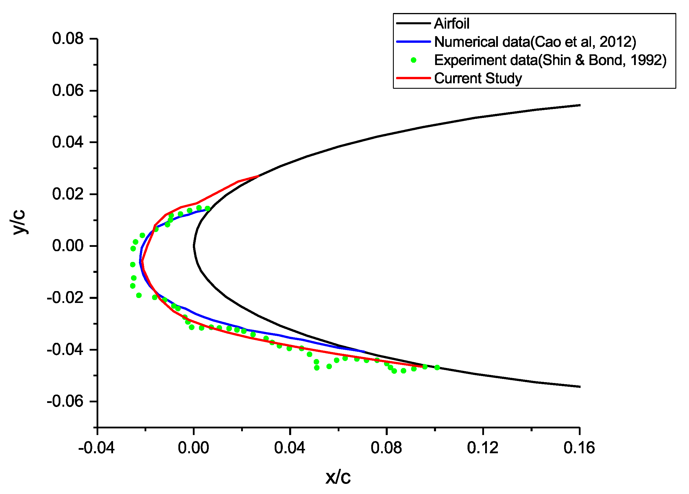
Changing the aircraft angle of attack affects the water droplets impingement location, collection efficiency distribution and the ice shape. Li et al. [14] developed a simulation framework to effectively study the ice accretion under a different angle of attack. It was found that when the wing is at a 4° angle of attack, the main impingement region is the lower surface of the wing. The same phenomenon is also observed in the ice height distribution, as shown in Figure 1 [14], with more ice accreted in the lower region. The black line represents the clean airfoil shape, the green dots represent the ice shape obtained in the experiment [32] and the blue and red solid lines represent the numerical predicted ice shape in Cao [12] and Li’s [14] work, respectively.
Exposure time is the time that an aircraft spent in the icing condition. It directly affects the ice shape and the longer a flight stays in icing condition, the more severe the icing severity is. During flight, the exposure time is directly related to the cloud size [33].
Liquid water content (LWC) is normally expressed as the number of grams of liquid water per cubic meter of air. It represents the amount of supercooled water droplets that can impact on the aircraft surface in a given air mass. Therefore, LWC is an important factor in aircraft icing. As LWC increases, the amount of ice and ice thickness also increase, which cause more severe damage to the flight safety.
A water droplet’s mass is directly proportional to the cube of the droplet diameter. Due to higher inertia, the droplets with higher diameter will be more likely to impact on the aircraft surface. On the other hand, smaller droplets tend to follow the air streamlines and avoid impacting on the surface. Therefore, the droplet diameter can affect the ice shape and ice layer thickness. The water droplet diameter is usually characterized as median volumetric diameter (MVD). According to the FAR-25 [33], the LWC and MVD is closely related; the relationship depends on the cloud type and environmental temperature. Therefore, at different temperatures, the distribution of LWC and MVD varies. The environmental temperature also affects the ice type. For example, it is more likely to form rime ice when the environmental temperature is low enough to make the entire water droplet to become frozen immediately upon the impact. On the other hand, glaze ice is more likely to be created when the water droplets only partially freeze [3].
2.3. Aircraft Icing Severity Levels
Defining the aircraft icing severity levels is important to give pilots a good idea how hazardous the icing is. The Aeronautical Information Manual [34] introduces four icing severity levels: trace, light, moderate and severe. However, since it simply serves as a reference for the pilots to give icing severity to the control tower, its classification is qualitative and vague. Later on, the NCCAM icing standard [35] defines the classification based on the accretion rate on a small probe (Table 1). Similarly, a icing severity level, as shown in Table 2, is established based on the maximum ice thickness [32]. Four levels are introduced to describe the icing severity, including light, moderate, heavy and severe. The pilots could use the standard as a reference to assess the severity of the flight condition [36]. It is reasonable to establish the standard based on the maximum ice thickness instead of the ice accretion rate because, during flight, the aircraft safety will only be a little affected if the time spent in severe icing state is limited.
3. Numerical Simulation for Aircraft Icing
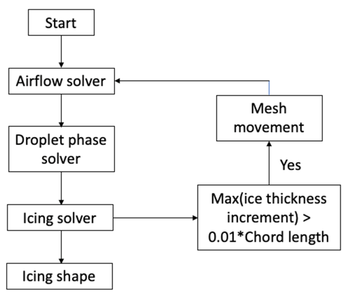
Since the flight test and experimental simulations are expensive to carry out, numerical simulation is adopted widely. There have been numerous discussions about the numerical tools to predict the ice accretion under different flight conditions [7,13,14,15]. The computational method proposed by Li et al. [14] for aircraft icing includes four main steps:
- Solve the air flow field around the aircraft.
- Simulate the droplet impingement on the aircraft surface.
- Solve the ice accretion model to compute the ice shape.
- Apply mesh morphing algorithm to account for the shape change caused by ice accretion.
The four steps construct the conventional icing simulation framework. This numerical tool is able to predict the ice shape as well as the effect of ice accretion on the aerodynamics performance. The framework is presented in Figure 2.
3.1. Airflow Field
Solving the airflow field is the first step in the ice accretion numerical modeling framework. The airflow field will affect the movement of the supercooled water droplets via drag force. The airflow field can be obtained by solving the potential flow equation [38] or the Euler equations [39] or the Navier–Stokes equations [14]. For example, the potential flow equation is solved in LEWICE code [7]. Cao et al. [13] solve the Eulerian equations to obtain the airflow field. Li et al. [14] solve the compressible Navier–Stokes equations based on the OpenFOAM framework [16,40]. Generally speaking, the Navier–Stokes is more complex to solve; however, the airflow field obtained by solving Navier–Stokes is more accurate, especially in the icing simulation where complex flow behavior often occurs. By solving the airflow field, the air flow velocity, pressure and temperature distribution is obtained and passed to the droplet impingement simulation.
3.2. Droplet Impingement
In the droplet impingement simulation, the crucial quantity that needs to be determined is the water droplet collection efficiency which reflects how often the droplets impact on the aircraft surface. The calculation of droplet collection efficiency on the airfoil/wing surface is crucial in numerically simulating ice accretions. The most natural technique to track the droplet motion is to individually compute the trajectory of each droplet, which is referred as Lagrangian method [41]. The Lagrangian method is easy to implement; however, it has a severe drawback in icing simulations, which is the enormous computational cost required to model the droplets. Another computational method available is Eulerian two-phase flow method [14]. Eulerian two-phase model considers the droplets in the airflow as continuous field which interpenetrates with the air. The collection efficiency is obtained through solving the droplet velocity and droplet volume fraction. The computational grid used in the airflow field simulation can be used for the Eulerian two-phase model, which further improved the efficiency. Eulerian two-phase model has been applied in many studies to simulate the droplet impingement [12,14,15].
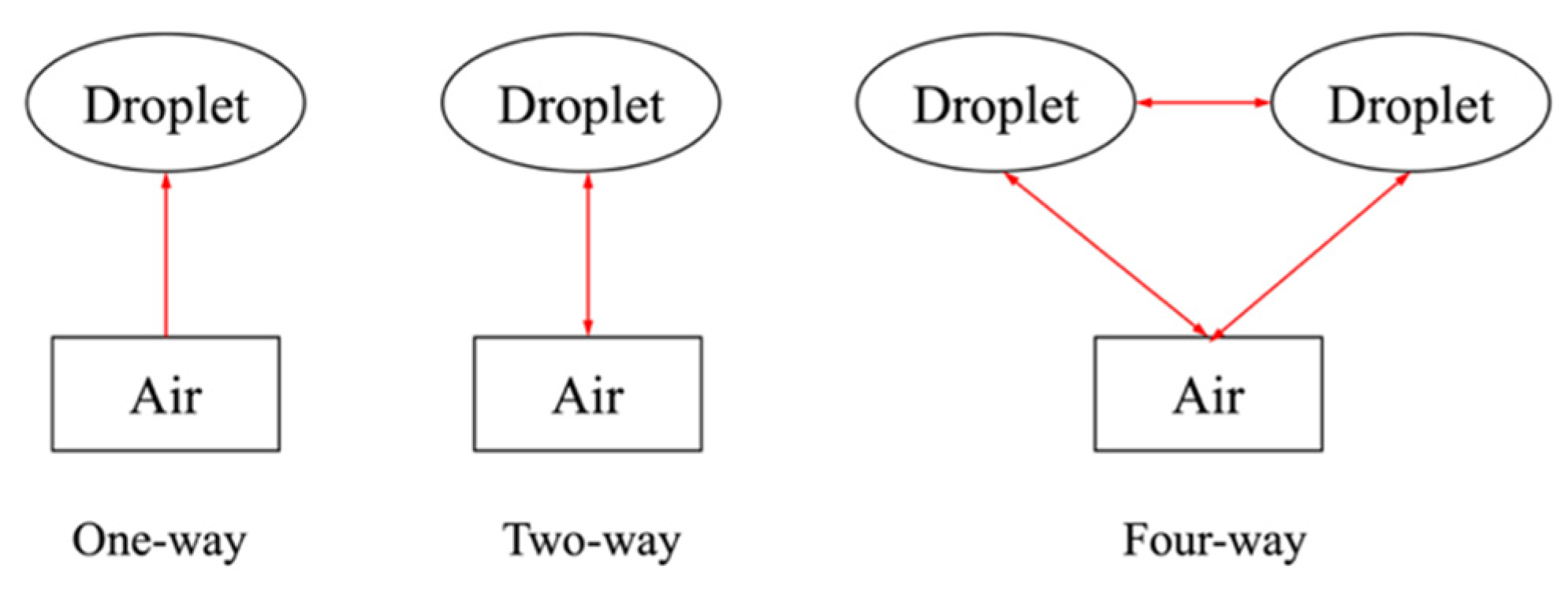
When applying the Eulerian two-phase model, different levels of interaction between air and droplets can be defined, as shown in Figure 3. The simplest model is one-way interaction in which only the airflow field affects the droplet phase. The most complex one is the four-way interaction where not only two-way interaction between air and droplets exist but the collision effect between droplets is considered as well. In many icing conditions, the droplet volume fraction is below 10−6; thus, one-way interaction is accepted [42].
In constructing the governing equations for the Eulerian two-phase model, the following assumptions [14] need to be made.
- The distribution of the water droplets is uniform, and they are simplified as sphere with a median volumetric diameter.
- The physical parameters of the droplets do not change by assuming that there is no heat or mass transfer between the droplets and air.
- The droplet collision, splashing and bouncing effects are neglected.
- The airflow viscosity has no effect on the droplets.
3.3. Ice Accretion
Many numerical approaches [7,12,13,14] apply the Messinger model [9] to solve the ice accretion process. The Messinger model constructs the mass balance and energy balance equations in the control volume on the aircraft surface based on the following assumptions [14].
- There is no runback water in the control volume at the stagnation point, and any runback water flowing out of the control volume flows along the direction away from the stagnation point.
- The heat and mass transfer only happens in the direction normal to the wing’s surface.
- In the mixture of water and ice, a balance temperature is reached.
As shown in Figure 4 [14], the mass coming into the control volume includes impinging water droplets, , and the water flow into the control volume from the upstream adjacent cell, . The mass going out of the control volume consists of the generated ice, , the evaporation or sublimation, , and the water flow out of the control volume to the downstream adjacent cell, . The mass balance equation can be written as
3.4. Mesh Morphing
Ice accretion changes the wing’s shape, which affects the previously solved airflow field and droplet impingement in step 1 and step 2 of the ice accretion numerical modeling framework. Therefore, it is necessary to re-calculate the airflow field and droplet flow field in order to obtain the new ice shape accurately based on the updated mesh. The irregular ice shape represents a major challenge in numerical simulation of long-time icing because manually remeshing is a time-consuming procedure. Kinzel et al. [43] use the mesh generation tool, AFLR3, to achieve the automated re-gridding procedure. Li et al. [14] build a mesh morphing algorithm to move the internal mesh nodes to achieve a smooth transition and maintain the mesh quality after constructing the ice shape.
4. Data-Driven Modeling for Aircraft Icing
This section details the different types of ML and then presents prominent research and findings of ML applications in aircraft icing. As described in the previous section, the aircraft icing process is a complex interaction of multiple variables and explicitly modeling the icing formation process often requires computationally expensive and/or cumbersome treatments to calculate the ice displacement and accretion along the wing, such as remeshing [22]. Data-driven methods can help alleviate this constraint by applying regression analysis and machine learning models to predict the aircraft icing based on icing data collected in experimental campaigns and/or numerical simulations [24]. Within the domain of aircraft icing, ML is applied in two main areas: ice shape prediction and icing severity evaluation.
4.1. Machine Learning
Since the ice accretion process shows strong nonlinearity, linear algorithms such as linear regression [44] and logistic regression [45] are not suitable [24]. Common nonlinear algorithms include the classification and regression trees (CART) [46], Naïve Bayes (NB) [47], k-Nearest Neighbors (KNN) [48] and Support Vector Machines (SVM) [49]. CART is referred to as decision tree (DT) algorithms that can be used for classification or regression predictive modeling problems. DT is a supervised learning method which can be used to make predictions in both regression and classification problems. DT constructs a binary tree from the training data, and the goal is to predict values by learning simple decision rules inferred from the data features. A tree can be seen as a piecewise constant approximation, and the split points are chosen greedily to minimize a cost function, such as Gini index [46]. The recursive binary splitting procedure needs to know when to stop splitting. The most common stopping criteria is the number of training instances assigned to each leaf node, whose value should be carefully tuned during the training process to avoid overfitting. Naïve Bayes calculates the probability of each class based on the Bayes theorem. It computes the conditional probability of each class given each input value based on the assumption of conditional independence between every pair of features given the value of the class variable. KNN is implemented through the instance bases learning with parameter k, which uses a majority voting mechanism [48] to make predictions in both regression and classification problems. One critical step in KNN is to determine which of the k instances in the training dataset are most similar to a new input. The common way is to use a distance measure, such as Euclidean distance and Hamming Distance. SVM seeks a line that best separates two classes. The optimal line will have the largest margin, which is the distance between the line and the closest data points. In practice, the SVM algorithm is implemented using a kernel, such as linear kernel and polynomial kernel, which defines the similarity or a distance measure between new data and the support vectors.
Besides the conventional ML models mentioned above, ensemble machine learning algorithms are also widely used in aircraft icing applications [24,26]. Ensemble ML methods create multiple models and then combine them to generate improved prediction results [50]. Li and Paoli [51] investigated the effectiveness of different conventional and ensemble ML methods on the icing applications. Ensemble methods usually have stronger prediction power and produce more accurate solutions than a single model would. Random Forest (RF) [52] is a type of ensemble method. RF constructs a set of decision trees during training, each individual tree gives a class prediction and the class that has the most votes becomes the model’s prediction. XGBoost is another ensemble model, which shows excellent performance on structured or tabular datasets on classification and regression predictive modeling problems [53]. In XGBoost, models are added sequentially, and new models are added to correct the errors made by existing models. Additionally, to avoid overfitting, XGBoost adds the regularization factor to the loss, which represents the complexity of the trees. It has been shown that XGBoost has promising performance in exploring the complex pattern between different types of icing conditions [26].
4.2. Machine Learning for Ice Shape Prediction
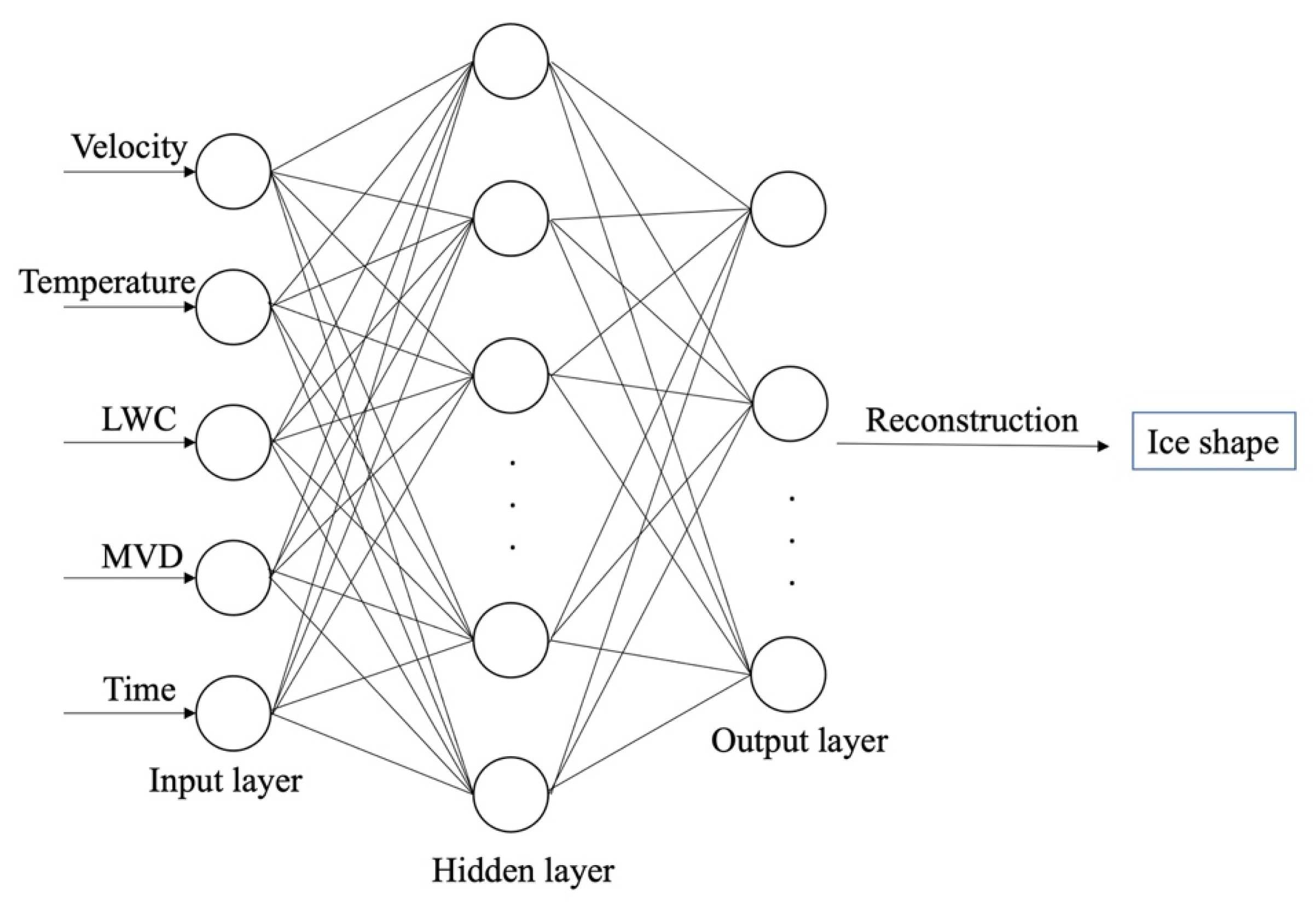
In aircraft icing, one of the applications of ML is to predict the ice shape. Predicting ice shape by using numerical simulation approach generally requires solving the partial different equations, which requires high computational cost. Many studies have been carried out to develop ML data-driven models as an alternative to the traditional numerical simulation approach. Ogretim et al. [25] incorporate the Fourier series expansion of an ice shape following a conformal mapping, which suppresses the effect of airfoil geometry, and then utilize neural networks to model the Fourier coefficients and the downstream extent of the ice shape. A set of 20 Fourier terms is given to the network. The training data for the NNs were generated at the NASA Icing Research Tunnel at NASA Glenn, which was reported in the LEWICE validation report [54]. Neural networks (NNs) have been widely used in supervised learning; an input space is mapped onto an output space through the constructed hidden layers [55]. The small computational resource requirement and reasonable accuracy make this method a promising alternative to the numerical simulation approach. NNs can also be combined with wavelet packet transform (WRT) to predict the ice shape [56]. Chang et al. [56] selected five variables (velocity, temperature, liquid water content, median volumetric diameter and exposure time) as input data and WRT is applied to reduce the number of input vectors to increase the convergence efficiency. The number of training samples is 43. Then, a back propagation network that consists of 1 hidden layer with 39 nodes is established, and the output coefficients are reconstructed to generate ice shape. The neural network schematic diagram is shown in Figure 6. The hyperbolic tangent sigmoid transfer function is used in the hidden layer, and the linear function is used in the output layer.
4.3. Machine Learning for Icing Severity Prediction
In aircraft icing severity evaluation, the use of ML methods has been shown to aid in reducing the computational time, enabling aircraft safety improvement. Li et al. [24] proposed a method for aircraft icing severity prediction at different flight conditions based on machine learning model XGBoost. Based on the numerical modeling, six flight conditions (flight speed, angle of attack, exposure time, LWC, MVD and freestream temperature) are considered as input to the ML model. A total of 1890 samples are selected to form the dataset. The model is trained to predict three icing severity features: the size of the area on the airfoil covered by ice, maximum ice thickness and icing severity level (Table 2). During the training process, an important step is to find the optimal parameter settings for the ML models. A scikit-learn class called “GridSearchCV” [57] can be applied to identify the optimal hyperparameter set to improve the prediction accuracy of the ML models. For example, in predicting the icing severity level using XGBoost [24], the number of trees is 80, interaction depth is 10, shrinkage factor is 0.1, subsample ratio is 1 and minimum child weight is 0.1. In order to evaluate the models’ performance, multiple statistical measures can be applied. For regression problems, the Root Mean Square Error (RMSE) [26], coefficient of determination R2 [26] and Median Absolute Error (MAE) [24] can be applied.
where is the number of data samples, and represent the value predicted by the model and the value prepared in the dataset, respectively.
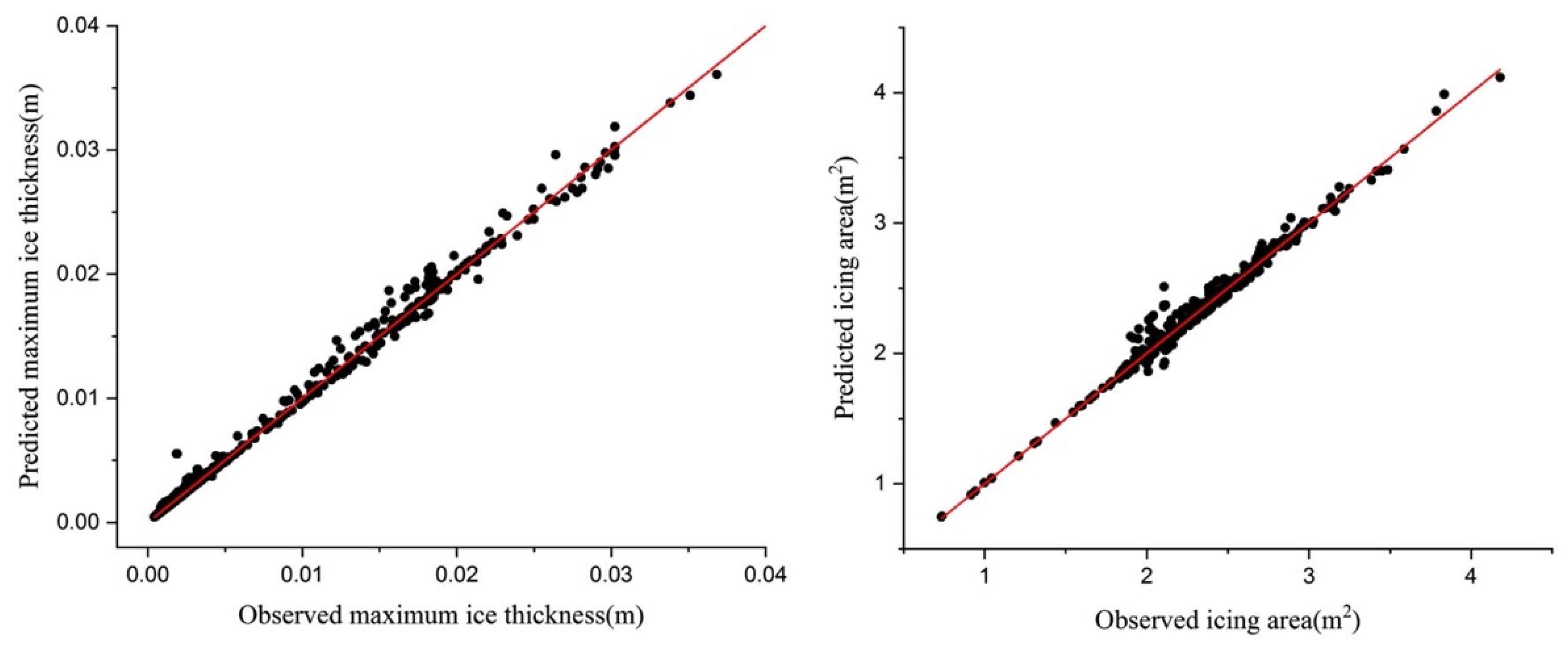
For classification problems, several model evaluation indicators, such as precision, recall rate, F1 score and confusion matrix, can be applied [26]. Figure 7 shows the comparison between the observed results and predicted results. The red line has an intercept of zero and a slope of one, which represents a perfect prediction. It can be observed that the sufficient agreement is achieved between the predicted and observed results in predicting the maximum ice thickness and icing area. The R2 computed from Figure 6 is 0.995 for both cases. Due to the low computational cost requirement and skillful prediction, some potential uses for this prediction model include the following:
- The proposed method has the potential to be coupled with other ice protection systems to further increase the flight safety, such as being an ice protection mechanism trigger.
- The hybrid machine learning and CFD methods can be applied to the estimation of the degradation of the aircraft performance.
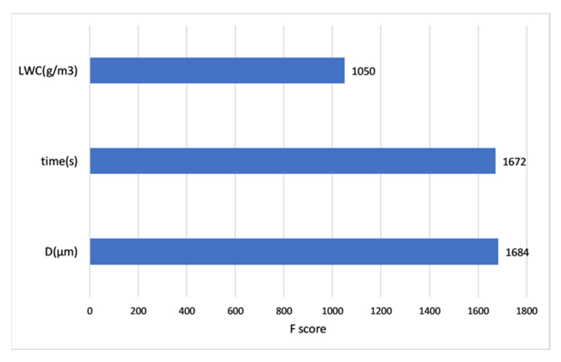
The built model can also output feature importance to indicate how valuable each flight condition is toward the three icing severity features. As an example, Figure 8 presents the feature importance of LWC, exposure time and droplet diameter in regard to the icing severity level. The F score value indicates how useful each feature is in the model building process. The higher the F score is, the more important the feature is. It can be seen that exposure time and droplet diameter have a comparable level of importance, while LWC has the lowest importance with regards to icing severity level.
Cao et al. [27] developed a methodology for predicting the effects of ice shape on airfoil aerodynamic performance based on a feed-forward neural network (NN). The model considers multiple ice geometry features, including ice horn leading-edge radius, ice height and ice horn position on airfoil surface. The model is trained to predict the lift coefficient, drag coefficient and moment coefficient, which are critical aerodynamic coefficients toward flight safety. Due to the sufficient agreement with the tunnel test data, the model can be further developed as a research tool to evaluate airfoil performance in different ice cloud conditions. McCann [37] built a pair of neural networks (NNICE) to recognize vertical atmospheric patterns associated to different icing intensities. A total of 398 samples are prepared for training the network. NNICE includes not only temperature and relative humidity at the flight level but also humidity data above and below flight level and a profile of the potential instability; therefore, it can make icing forecasts of all intensities with reasonable accuracy.
5. Conclusions and Prospects
Aircraft icing has been studied by numerical modeling and machine learning methods. In research, numerical simulation has been shown to be effective in calculating the ice shape, analyzing the detailed flow fields and predicting the effect of ice shape on aerodynamics. The highly modular structure of the numerical simulation framework can easily incorporate different CFD and ice accretion models to provide more in-depth analysis. ML has been successfully used to accelerate the ice shape prediction process and enable fast evaluation of aircraft icing severity. The ability of ML models to generate the feature importance can help to study the effect of different aerodynamic and meteorological factors on the icing severity results. Due to the small computational resource requirement, fast performance and reasonable accuracy, the ML models can provide an attractive alternative to the traditional numerical simulation approach. Additionally, the ML models have the potential to be coupled with CFD codes and ice protection system to further increase the flight safety. Accurate data, such as those from high-fidelity CFD simulation, would help build useful training datasets for ML developments, especially for unsteady flows that occur in certain phases and/or specific wing configurations (flap deployment, retraction).
Author Contributions
Conceptualization, S.L. and R.P.; methodology, S.L. and R.P.; software, S.L.; validation, S.L.; formal analysis, S.L.; investigation, S.L. and R.P.; resources, R.P.; data curation, S.L.; writing—original draft preparation, S.L.; writing—review and editing, S.L. and R.P.; visualization, S.L.; supervision, R.P.; project administration, R.P.; funding acquisition, R.P. All authors have read and agreed to the published version of the manuscript.
Funding
This work was supported by Argonne National Laboratory through grant number ANL 0J-60008-0019A, titled “High-performance computing and physics-informed machine learning for multiscale flows”, and by National Science Foundation through grant number 1854815, titled “High-Performance Computing and Data-Driven Modeling of Aircraft Contrails,” awarded to R. Paoli.
Data Availability Statement
Data sharing not applicable.
Conflicts of Interest
The authors declare no conflict of interest.
Entry Link on the Encyclopedia Platform
References
- Mclean, J.J. Determining the effects of weather in aircraft accident investigations. In Proceedings of the 24th Aerospace Sciences Meeting, Reno, NV, USA, 6–9 January 1986. [Google Scholar] [CrossRef]
- Chang, L. Aircraft icing and aviation safety. Aeronaut. Sci. Technol. 2010, 5, 12–14. [Google Scholar]
- Cao, Y.; Tan, W.; Wu, Z. Aircraft icing: An ongoing threat to aviation safety. Aerosp. Sci. Technol. 2018, 75, 353–385. [Google Scholar] [CrossRef]
- Ratvasky, T.; Van Zante, J.; Riley, J. Thomas Ratvasky, “NASA/FAA Tailplane Icing Program overview”. In Proceedings of the 37th Aerospace Sciences Meeting and Exhibit, Reno, NV, USA, 11–14 January 1999. [Google Scholar]
- Papadakis, M.; Yeong, H.W.; Vargas, M.; Potapczuk, M. Aerodynamic Performance of a Swept Wing with Ice Accretions. In Proceedings of the 41st Aerospace Sciences Meeting and Exhibit, Reno, NV, USA, 6–9 January 2003. [Google Scholar] [CrossRef]
- Ratvasky, T.P.; Ranaudo, R.J. Icing Effects on Aircraft Stability and Control Determined from Flight Data, Preliminary Results. In Proceedings of the 31st Aerospace Sciences Meeting, Reno, NV, USA, 11–14 January 1993. No. NASA TM 105977. [Google Scholar]
- Ruff, G.; Berkowitz, B. User’s Manual for the NASA Lewis Ice Accretion Prediction Code (LEWICE); NASA: Washington, DC, USA, 1990.
- Wright, W.B. User Manual for the NASA Glenn Ice Accretion Code LEWICE, Ver. 2.2.2; NASA/CR-2002-211793; NASA: Washington, DC, USA, 2002.
- Messinger, B. Equilibrium temperature of an unheated icing surface as a functionof air speed. J. Aeronaut. Sci. 1953, 20, 29. [Google Scholar] [CrossRef]
- Beaugendre, H.; Morency, F.; Habashi, W.G. FENSAP-ICE’s three-dimensional inflightice accretion module: ICE3D. J. Aircr. 2003, 40, 239. [Google Scholar] [CrossRef]
- Mingione, G.; Brandi, V. Ice Accretion Prediction on Multielement Airfoils. J. Aircr. 1998, 35, 240–246. [Google Scholar] [CrossRef]
- Cao, Y.; Ma, C.; Zhang, Q.; Sheridan, J. Numerical simulation of ice accretions on an aircraft wing. Aerosp. Sci. Technol. 2011, 23, 296–304. [Google Scholar] [CrossRef]
- Cao, Y.; Huang, J.; Yin, J. Numerical simulation of three-dimensional ice accretion on an aircraft wing. Int. J. Heat Mass Transf. 2016, 92, 34–54. [Google Scholar] [CrossRef]
- Li, S.; Paoli, R. Modeling of Ice Accretion over Aircraft Wings Using a Compressible OpenFOAM Solver. Int. J. Aerosp. Eng. 2019, 2019, 4864927. [Google Scholar] [CrossRef]
- Li, S.; Paoli, R. Numerical Study of Ice Accretion over Aircraft Wings Using Delayed Detached Eddy Simulation. Bull. Am. Phys. Soc. 2019, 64, Q23-009. [Google Scholar]
- Weller, H.G.; Tabor, G.; Jasak, H.; Fureby, C. A tensorial approach to computational continuum mechanics using object-oriented techniques. Comput. Phys. 1998, 12, 620–631. [Google Scholar] [CrossRef]
- Gori, G.; Zocca, M.; Garabelli, M.; Guardone, A.; Quaranta, G. PoliMIce: A simulation framework for three-dimensional ice accretion. Appl. Math. Comput. 2015, 267, 96–107. [Google Scholar] [CrossRef]
- Fortin, G.; Laforte, J.-L.; Ilinca, A. Heat and mass transfer during ice accretion on aircraft wings with an improved roughness model. Int. J. Therm. Sci. 2006, 45, 595–606. [Google Scholar] [CrossRef]
- Han, Y.; Palacios, J. Surface Roughness and Heat Transfer Improved Predictions for Aircraft Ice-Accretion Modeling. AIAA J. 2017, 55, 1318–1331. [Google Scholar] [CrossRef]
- Spalart, P.R.; Deck, S.; Shur, M.L.; Squires, K.D.; Strelets, M.K.; Travin, A. A New Version of Detached-eddy Simulation, Resistant to Ambiguous Grid Densities. Theor. Comput. Fluid Dyn. 2006, 20, 181–195. [Google Scholar] [CrossRef]
- Xiao, M.; Zhang, Y. Improved Prediction of Flow Around Airfoil Accreted with Horn or Ridge Ice. AIAA J. 2021, 59, 2318–2327. [Google Scholar] [CrossRef]
- Li, S.; Paoli, R.; D’Mello, M. Scalability of OpenFOAM Density-Based Solver with Runge–Kutta Temporal Discretization Scheme. Sci. Program. 2020, 2020, 9083620. [Google Scholar] [CrossRef]
- Moacir, R.F.; Ponti, A. Machine Learning: A Practical Approach on the Statistical Learning Theory; Springer: Cham, Switzerland, 2018. [Google Scholar]
- Li, S.; Qin, J.; Paoli, R. Data-Driven Machine Learning Model for Aircraft Icing Severity Evaluation. J. Aerosp. Inf. Syst. 2021, 18, 876–880. [Google Scholar] [CrossRef]
- Ogretim, E.; Huebsch, W.; Shinn, A. Aircraft Ice Accretion Prediction Based on Neural Networks. J. Aircr. 2006, 43, 233–240. [Google Scholar] [CrossRef]
- Li, S.; Qin, J.; He, M.; Paoli, R. Fast Evaluation of Aircraft Icing Severity Using Machine Learning Based on XGBoost. Aerospace 2020, 7, 36. [Google Scholar] [CrossRef]
- Cao, Y.; Yuan, K.; Li, G. Effects of ice geometry on airfoil performance using neural networks prediction. Aircr. Eng. Aerosp. Technol. 2011, 83, 266–274. [Google Scholar] [CrossRef]
- Vukits, T. Overview and risk assessment of icing for transport category aircraft and components. In Proceedings of the 40th AIAA Aerospace Sciences Meeting & Exhibit, Reno, NV, USA, 14–17 January 2002. [Google Scholar] [CrossRef]
- Heinrich, A.; Ross, R.; Zumwalt, G.; Provorse, J.; Padmanabhan, V. Aircraft Icing Handbook; Federal Aviation Administration: Washington, DC, USA, 1993; Volume 1–3.
- Bragg, M.B. Rime Ice Accretion and Its Effect on Airfoil Performance. Ph.D. Thesis, Ohio State Univ., Columbus, OH, USA, September 1982. Available online: https://ntrs.nasa.gov/citations/19820016290 (accessed on 26 November 2021).
- Mikkelsen, K.; Mcknight, R.; Ranaudo, R.; Perkins, J.P. Icing flight research—Aerodynamic effects of ice and ice shape documentation with stereo photography. AIAA Pap. 1985, 85, 468. [Google Scholar] [CrossRef]
- Shin, J.W.; Bond, T.H. Experimental and Computational Ice Shapes and Resulting Drag Increase for a NACA 0012 Airfoil; National Aeronautics and Space Administration: Washington, DC, USA, 1992.
- F.A. Regulations, Part 25—Airworthiness Standards: Transport Category Air-planes; Federal Aviation Administration: Washington, DC, USA, 2013.
- Federal Aviation Administration. Aeronautical Information Manual (AIM), Updated Annually; Federal Aviation Administration: Washington, DC, USA, 2021.
- Mitchell, L.V. Aircraft Icing—A New Look. Aerosp. Saf. 1964, 9–11. [Google Scholar]
- McCann, D.W. NNICE—A neural network aircraft icing algorithm. Environ. Model. Softw. 2005, 20, 1335–1342. [Google Scholar] [CrossRef]
- Zhang, C. Flight Meteorology; Meteorological Press: Beijing, China, 2000. [Google Scholar]
- Chanson, H. Applied Hydrodynamics: An Introduction to Ideal and Real Fluid Flows; CRC Press Taylor & Francis Group: Lei-den, The Netherlands, 2009. [Google Scholar]
- Gibbon, J.D.; Moore, D.R.; Stuart, J.T. Exact, infinite energy, blow-up solutions of the three-dimensional Euler equa-tions. Nonlinearity 2003, 16, 1823–1831. [Google Scholar] [CrossRef]
- Li, S.; Qiao, H. Development of a Fast Fluid Dynamics Model Based on PISO Algorithm for Simulating Indoor Airflow. In Proceedings of the ASME 2021 Heat Transfer Summer Conference, HT 2021, Virtual, Online, 16–18 June 2021. [Google Scholar] [CrossRef]
- Hoffmann, L.D.; Bradley, G.L. Calculus for Business, Economics, and the Social and Life Sciences, 8th ed.; McGraw-Hill: New York City, NY, USA, 2004. [Google Scholar]
- Elghobashi, S. On predicting particle-laden turbulent flows. Flow Turbul. Combust. 1994, 52, 309–329. [Google Scholar] [CrossRef]
- Kinzel, M.P.; Noack, R.W.; Sarofeen, C.M.; Boger, D.; Kreeger, R.E. A CFD Approach for Predicting 3D Ice Accretion on Aircraft. In Proceedings of the SAE 2011 International Conference on Aircraft and Engine Icing and Ground Deicing, Chicago, IL, USA, 13–17 June 2011. [Google Scholar] [CrossRef]
- Darlington, R.B.; Hayes, A.F. “Multicategorical Regressors”, Regression Analysis and Linear Models: Concepts, Applications, and Implementation; Guilford Publications: New York, NY, USA, 2016. [Google Scholar]
- Harrell, F.E. Ordinal Logistic Regression. In Regression Modeling Strategies; Springer: Cham, Switzerland, 2015; pp. 311–325. [Google Scholar]
- Kamiński, B.; Jakubczyk, M.; Szufel, P. A framework for sensitivity analysis of decision trees. Central Eur. J. Oper. Res. 2017, 26, 135–159. [Google Scholar] [CrossRef] [PubMed]
- Webb, G.I.; Boughton, J.R.; Wang, Z. Not So Naive Bayes: Aggregating One-Dependence Estimators. Mach. Learn. 2005, 58, 5–24. [Google Scholar] [CrossRef]
- Altman, N.S. An Introduction to Kernel and Nearest-Neighbor Nonparametric Regression. Am. Stat. 1992, 46, 175. [Google Scholar] [CrossRef]
- Cortes, C.; Vapnik, V. Support-vector networks. Mach. Learn. 1995, 20, 273–297. [Google Scholar] [CrossRef]
- He, H.; Yang, Y.; Pan, Y. Machine learning for continuous liquid interface production: Printing speed modelling. J. Manuf. Syst. 2019, 50, 236–246. [Google Scholar] [CrossRef]
- Li, S.; Paoli, R. Comparison of Machine Learning Models for Data-Driven Aircraft Icing Severity Evaluation. J. Aerosp. Inf. Syst. 2021, 18, 973–977. [Google Scholar] [CrossRef]
- Breiman, L. Random Forests. Mach. Learn. 2001, 45, 5–32. [Google Scholar] [CrossRef]
- Chen, T.; Guestrin, C. XGBoost: A Scalable Tree Boosting System. In Proceedings of the 22nd ACM SIGKDD International Conference on Knowledge Discovery and Data Mining, San Francisco, CA, USA, 13–17 August 2016; pp. 785–794. [Google Scholar]
- Wright, W.B.; Rutkowski, A. Validation Results for LEWICE 2.0; NASA: Washington, DC, USA, 1999.
- Sosnovik, I.; Oseledets, I. Neural networks for topology optimization. Russ. J. Numer. Anal. Math. Model. 2019, 34, 215–223. [Google Scholar] [CrossRef]
- Chang, S.; Leng, M.; Wu, H.; Thompson, J. Aircraft ice accretion prediction using neural network and wavelet packet transform. Aircr. Eng. Aerosp. Technol. 2016, 88, 128–136. [Google Scholar] [CrossRef]
- Pedregosa, F.; Varoquaux, G.; Gramfort, A.; Michel, V.; Thirion, B.; Grisel, O.; Blondel, M.; Prettenhofer, P.; Weiss, R.; Dubourg, V. Scikit-Learn: Machine Learning in Python. J. Mach. Learn. Res. 2011, 12, 2825–2830. [Google Scholar]
Figure 1.
Visualization of the ice shape comparison on the NACA0012 airfoil [14].
Figure 1.
Visualization of the ice shape comparison on the NACA0012 airfoil [14].

Figure 2.
Ice accretion numerical modeling framework (* represents product of 0.01 and chord length).
Figure 2.
Ice accretion numerical modeling framework (* represents product of 0.01 and chord length).

Figure 3.
Different levels of interaction between air and droplet.

Figure 4.
Mass balance in the control volume [14].
Figure 4.
Mass balance in the control volume [14].

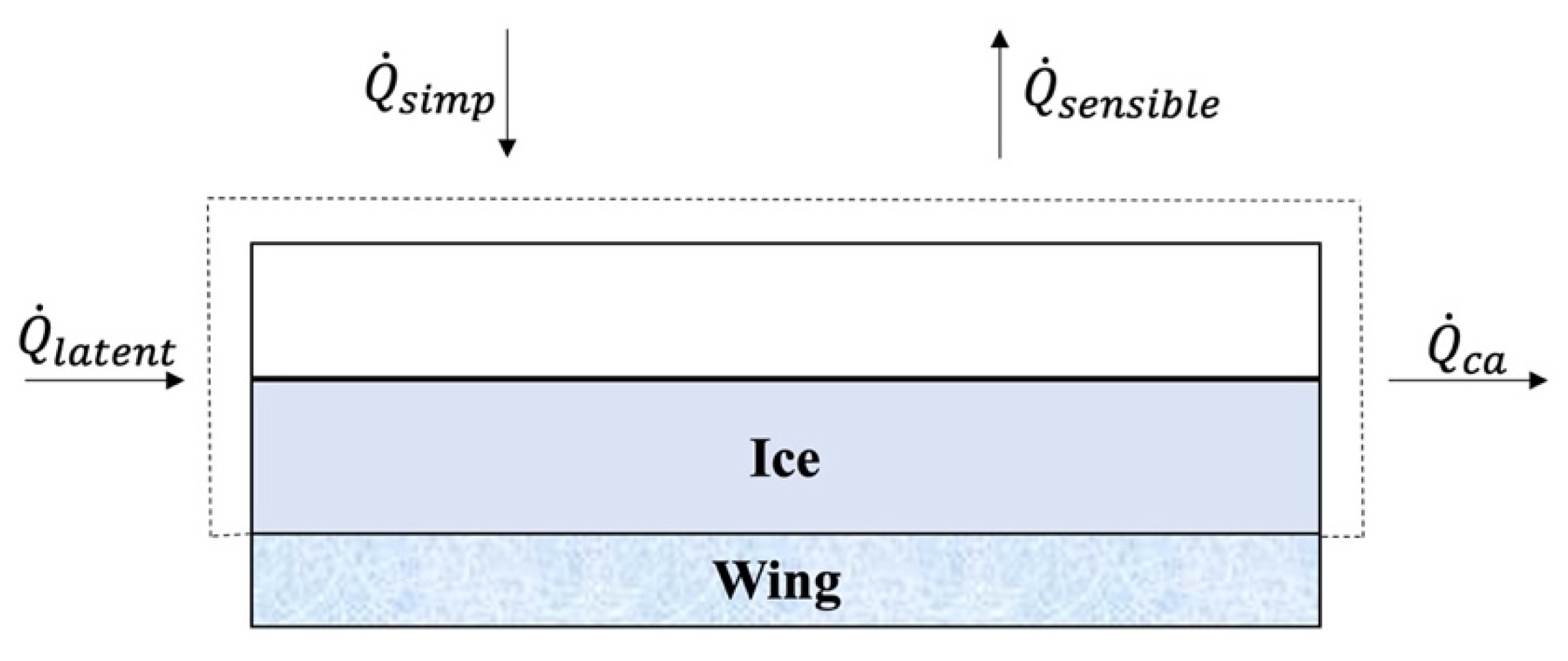
Figure 5.
Energy balance in the control volume [14].
Figure 5.
Energy balance in the control volume [14].

Figure 6.
Schematic diagram of neural network structure [55].
Figure 6.
Schematic diagram of neural network structure [55].

Figure 7.
Scatter plot of observed results vs. predicted results. Left panel: maximum ice thickness; right panel: icing area [24].
Figure 7.
Scatter plot of observed results vs. predicted results. Left panel: maximum ice thickness; right panel: icing area [24].

Figure 8.
Bar chart of XGBoost feature importance in regard to icing severity level prediction [26].
Figure 8.
Bar chart of XGBoost feature importance in regard to icing severity level prediction [26].


Table 1.
1964 NCCAM icing standards [35].
Table 1.
1964 NCCAM icing standards [35].
| Icing Severity Level | Accretion Rate on a Small Probe |
|---|---|
| Trace | 1/2 inch in 80 miles |
| Light | 1/2 inch in 40 miles |
| Moderate | 1/2 inch in 20 miles |
| Heavy | 1/2 inch in 10 miles |
Table 2.
Icing severity level based on icing thickness [37].
Table 2.
Icing severity level based on icing thickness [37].
| Icing Severity Level | Maximum Ice Thickness (mm) |
|---|---|
| Light | 0.1–5.0 |
| Moderate | 5.1–15 |
| Heavy | 15.1–30 |
| Severe | >30 |
Publisher’s Note: MDPI stays neutral with regard to jurisdictional claims in published maps and institutional affiliations. |
© 2022 by the authors. Licensee MDPI, Basel, Switzerland. This article is an open access article distributed under the terms and conditions of the Creative Commons Attribution (CC BY) license (https://creativecommons.org/licenses/by/4.0/).
Share and Cite
MDPI and ACS Style
Li, S.; Paoli, R. Aircraft Icing Severity Evaluation. Encyclopedia 2022, 2, 56-69. https://0-doi-org.brum.beds.ac.uk/10.3390/encyclopedia2010005
AMA Style
Li S, Paoli R. Aircraft Icing Severity Evaluation. Encyclopedia. 2022; 2(1):56-69. https://0-doi-org.brum.beds.ac.uk/10.3390/encyclopedia2010005
Chicago/Turabian StyleLi, Sibo, and Roberto Paoli. 2022. "Aircraft Icing Severity Evaluation" Encyclopedia 2, no. 1: 56-69. https://0-doi-org.brum.beds.ac.uk/10.3390/encyclopedia2010005