STL Decomposition of Time Series Can Benefit Forecasting Done by Statistical Methods but Not by Machine Learning Ones ^†

Abstract

This paper aims at comparing different forecasting strategies combined with the STL decomposition method. STL is a versatile and robust time series decomposition method. The forecasting strategies we consider are as follows: three statistical methods (ARIMA, ETS, and Theta), five machine learning methods (KNN, SVR, CART, RF, and GP), and two versions of RNNs (CNN-LSTM and ConvLSTM). We conduct the forecasting test on six horizons (1, 6, 12, 18, and 24 months). Our results show that, when applied to monthly industrial M3 Competition data as a preprocessing step, STL decomposition can benefit forecasting using statistical methods but harms the machine learning ones. Moreover, the STL-Theta combination method displays the best forecasting results on four over the five forecasting horizons.

1. Introduction

Time series forecasting is a subdomain of time series analysis in which the historical measurements are modeled to describe the underlying characteristics of the observable and extrapolated into the future [1].

For a few decades, the domain of time series analysis has been dominated by statistical methodology. One of the most important and generally used models is the AutoRegressive Integrated Moving Average (ARIMA), which can be quickly built thanks to the Box–Jenkins methodology [2]. The ARIMA family has excellent flexibility for presenting varying time series. Nevertheless, it has limits due to its assumption of linearity of the time series [1,3].

Another dominating and widely used statistical method is the ExponenTial Smoothing (ETS) method, which was proposed in the 1950s [4,5,6]. It is often considered as an alternative to the ARIMA models. While the ARIMA family develops a model where the prediction is a weighted linear sum of recent past observations or lags, forecasts produced by ETS are weighted averages of past observations, with the weights decaying exponentially as the observations get older [7].

The M Competitions were initiated by professor Spyros Makridakis. There are different open competitions (M1–M5) dedicated to the performance comparison of different forecasting methods [8]. Particularly, the Theta method had impressive success in the M3 Competition and thus was used in the M4 Competition as a benchmark. It was first proposed by Assimakopoulos et al. [9] and then extended to forecast multivariate macroeconomic and financial time series [10]. Hyndman demonstrated the Theta method applied in the M3 Competition is equivalent to the simple exponential smoothing with a drift [11].

Time series can also have many underlying patterns, and decomposition can reveal them by splitting a time series into several components. In our study, we focus on STL decomposition. STL stands for Seasonal-Trend decomposition using LOESS, where LOESS is LOcal regrESSion, which was proposed by Robert et al. in 1990 [12], contributing to a decomposition method robust to anomalies.

Artificial Intelligence (AI) has gained significant prominence over the last decade, especially in object recognition [13], natural language processing (NLP) [14], and autonomous driving [15]. Convolutional Neural Networks (CNNs) have revolutionized the field of computer vision [16]. Recurrent Neural Networks (RNNs) benefited from lots of NLP tasks, such as machine translation [17] and speech recognition [18]. In the field of time series, many machine learning methods such as support vector regression (SVR), neural networks, classification and regression tree (CART), and k-nearest neighbor (kNN) regression were proven able to model and forecast time series as well [19,20].

There are some discussions on comparing the performance of different forecasting approaches. Ahmed et al. [21] performed an empirical comparison of eight machine learning models over the 1045 monthly series involved in the M3 Competition, but only one-step-ahead forecasting was considered. Makrirdakis et al. did some similar works [22], comparing statistical and machine learning methods, but without any decomposition method being introduced as a preprocessing step. Using the M1 Competition dataset, Theodosieu [23] compared a new STL-based method with some common benchmarks but without combining STL with them, and only up to an 18-month forecasting was considered.

As the preprocessing step often plays an integral part in prediction tasks and substantially impacts the results, we propose to conduct a new comparison work to identify its benefit: (1) by exploring STL decomposition when using it as a preprocessing step for all methods; and (2) by considering multiple forecasting horizons.

The rest of this paper is organized as follows. In the next section, we present a concise description of all the involved models and the decomposition methods. Section 3 presents how we organized and conducted the experiments. In Section 4, we present the comparison results and discussions based on these results. Section 5 gives the conclusion.

2. Methods

Although there are many different variations of each model, we considered only the primitive versions of each model in our experiments. As this paper is inspired heavily by the M3 and M4 Competitions, we kept the six benchmark methods used in these two competitions by the organizer [24].

2.1. Existing Benchmarks in M4 Competitions

Below is a list of descriptions of the benchmarks utilized in the M4 Competition.

• Naïve 1. Naïve 1 assumes future values are identical to the last observation.
• Naïve S. Naïve S assumes future values are identical to the values from the last known period, which, in our case, is 12 months.
• Naïve 2. Naïve 2 is similar to Naïve 1, except the data are seasonally adjusted by a conventional multiplicative decomposition if tested seasonal. We performed a 90% autocorrelation test at lag 12 for each series.
• Simple Exponential Smoothing (SES). SES forecasts future values as exponentially decayed weighted averages of past observations [7].
• Holt. Holt’s linear trend method extends SES for data with a trend [7].
• Damped. The damped model dampens the trend in Holt’s method [7].

2.2. Conventional Decomposition and STL Decomposition

Here, we introduce two commonly used decomposition methods.

2.2.1. Conventional Decomposition

The conventional multiplicative classical decomposition algorithm for a series with seasonal period m has four steps [7]:

• Compute the trend component ${\widehat{T}}_t$ using a simple moving average method.
• Detrend the time series: $y_t/{\widehat{T}}_t$.
• Compute the seasonal component ${\widehat{S}}_t$ by averaging the corresponding season’s detrended values and then adjusting to ensure that they add to m.
• Compute the remainder component ${\widehat{R}}_t$: ${\widehat{R}}_t=y_t/\left({\widehat{T}}_t{\widehat{S}}_t\right)$.

2.2.2. STL Decomposition

STL decomposition consists of two recursive procedures: an inner loop and an outer loop. The inner loop fits the trend and calculates the seasonal component. Every inner loop consists of six steps in total:

• Detrending. Calculate a detrended series $y_v-T_v^{\left(k\right)}$. For the first pass, $T_v^{\left(0\right)}=0$.
• Cycle-Subseries Smoothing. Use LOESS to smooth the subseries of values at each position of the seasonal cycle. The result is marked as $C_v^{(k+1)}$.
• Low-Pass Filtering of Smoothed Cycle-Subseries. This procedure consists of two MA filters and a LOESS smoother. The result is marked as $L_v^{(k+1)}$.
• Detrending of Smoothed Cycle-Subseries. $S_v^{(k+1)}=C_v^{(k+1)}-L_v^{(k+1)}$.
• Deseasonalizing. $y_v-S_v^{(k+1)}$.
• Trend Smoothing. Use LOESS to smooth the deseasonalized series to get the trend component of this pass $T_v^{(k+1)}$.

If any anomaly is detected, an outer loop will be applied and replace the LOESSs at the second and sixth steps of the inner loop with the robust LOESS.

2.3. ARIMA, ETS, and Theta

• ARIMA. An ARIMA model assumes future values to be linear combinations of past values and random errors, contributing to the AR and MA terms, respectively [2]. SARIMA (Seasonal ARIMA) is an extension of ARIMA that explicitly supports time series data with a seasonal component. Once STL decomposition is applied, SARIMA models degenerate into regular ARIMA models as STL handles the seasonal part.
• ETS. The ETS models are a family of time series models with an underlying state space model consisting of a level component, a trend component (T), a seasonal component (S), and an error term (E). Forecasts produced using exponential smoothing methods are weighted averages of past observations, with the weights decaying exponentially as the observations get older [7]. After concatenating STL on the ETS model, the full ETS model degenerates into Holt’s method [7] as the seasonal equation is handled by STL.
• Theta Method. The Theta method, initially proposed in 2000 by Assimakopoulos et al. [9], performed exceptionally well in the M3 Competition and was used as a benchmark in the M4 Competition. The Theta method is based on the concept of modifying the local curvature of the time series through a coefficient $\theta$, which is applied directly to the second difference of the data [9]. Hyndman demonstrated that the h-step-ahead forecast obtained by the Theta method is equivalent to an SES with drift depending on the smoothing parameter value of SES, the horizon h, and the data [11].

2.4. Machine Learning Methods

It is interesting to closely examine how machine learning methods perform in time series forecasting tasks. Using the embedding strategy to transform this task into a supervised learning problem [25], we can apply machine learning techniques to time series forecasting tasks. The following briefly introduces the machine learning methods used in this experimentation.

• $\mathit{k}$-NN.k-NN is a non-parametric method used for classification and regression. In both cases, the input consists of the k closest training examples in the feature space. In k-NN regression, the output is the property value for the object. This value is the average of the values of k nearest neighbors based on the Euclidian distances.
• SVR. Support Vector Machine (SVM) is a successful method that tries to find a separation hyperplane to maximize the margin between two classes, while SVR seeks a hyperplane to minimize the margin between the support vectors and the hyperplane.
• CART. CART is one of the most generally used machine learning methods and can be used for classification and regression. CART dichotomizes each feature recursively and divides the input space into several cells. CART computes the probability distributions of the corresponding prediction in it.
• RF. RF is an ensemble learning algorithm based on the Decision Tree [26]. Similar to CART, Random Forest can be used for both classification and regression. It operates by constructing many decision trees at training time and calculating the average predictions from the individual trees.
• GP. A GP is a generalization of the Gaussian probability distribution [27]. It uses a measure of homogeneity between points as a kernel function to predict an unknown point’s value from the input training data. The result of its prediction contains the value of the point and the uncertainty information, i.e., its one-dimensional Gaussian distribution [22].

2.5. Deep Learning Methods

For the promising capacity of RNNs to memorize the long-term values, we decided to test the deep learning models. Here, we present two structures of RNNs implemented in our experimentation. The first one is the well-known CNNs stacked with the Long Short-Term Memory (LSTM) cells, and the other one is the ConvLSTM structure proposed by Xingjian Shi et al. in NeurIPS 2015 [28].

• CNN-LSTM. We use a 1D CNN to handle univariate time series. It has a hidden convolutional layer iterating over a 1D sequence and follows a pooling layer to extract the most salient features, which is then interpreted by a fully connected layer. Then, we stack it with some LSTM layers, which is a widely used RNNs model that provides a solution to the vanishing gradient problem for RNNs. It was proposed by Sepp Hochreiter et al. in 1997 [29].
• Convolutional LSTM (ConvLSTM). ConvLSTM is an RNNs with convolutional structures in both the input-to-state and state-to-state transitions. It determines the future state of a certain cell in the grid by its local neighbors’ inputs and past states. This is achieved using a convolution operator in the state-to-state and input-to-state transitions [28]. Rather than reading and extracting the features with a CNN and then interpreting them by an LSTM, ConvLSTM reads and interprets them at a time.

3. Experimentation Setup

This section presents how we organized and performed our experimentation.

3.1. Dataset

We selected 332 monthly series from the industry category which contains the highest number of points per series from the M3 Competition dataset. We set 84 as the length of the historical data and tested five different forecast horizons, i.e., 1, 6, 12, 18, and 24 months. Thus, the total length required for an appropriate series is 108. The two series N2011 (78 points) and N2118 (104 points) were thus removed from the original 334-series dataset.

3.2. Pipeline for Machine Learning and Deep Learning Methods

3.2.1. Data Preprocessing

In our experimentation, three preprocessing techniques were conducted on all the series:

• Deseasonalizing: A 90% autocorrelation test at lag 12 is performed to decide whether the series is seasonal. We perform a conventional multiplicative decomposition or an STL decomposition if the series is seasonal and extract the seasonal part.
• Detrending: A one-order differencing is performed to eliminate the trend.
• Scaling: A standardization step is applied to remove the mean and scale the features to unit variance.

3.2.2. Supervised Learning Setting

A time series prediction problem can be transformed into a supervised learning task that machine learning and deep learning methods can do. A commonly used approach is to formulate a training set by lagging and stacking the historical series several times, which is often referred to as the embedding technique in the R implementation [30].

Typically, for an h-step-ahead prediction problem, we can construct a training set $\{X,Y\}$ as follows:

$$X=\left[\begin{array}{cccc}{y}_1& y_2& \cdots & y_n\\ y_2& y_3& \cdots & y_{n+1}\\ ⋮& ⋮& ⋮& ⋮\\ y_{N-n-h+1}& y_{N-n-h+2}& \cdots & y_{N-h}\end{array}\right],Y=\left[\begin{array}{cccc}{y}_{n+1}& y_{n+2}& \cdots & y_{n+h}\\ y_{n+2}& y_{n+3}& \cdots & y_{n+h+1}\\ ⋮& ⋮& ⋮& ⋮\\ y_{N-h+1}& y_{N-h+2}& \cdots & y_N\end{array}\right],$$

(1)

where N is the total length of the series, n is the number of times we lag the series, often referred to as the window length. Each row in X represents a training example, while its label corresponds to the vector in the same row in Y.

3.2.3. Results Post-Processing

The post-processing part comprises the inverted operations of the three preprocessing steps:

• Rescaling: A rescaling step is performed by inverting the standardization.
• Retrending: A cumulated summing is conducted to bring back the trend.
• Reseasonalizing: A reseasonalization step is executed to integrate the seasonal component into the prediction.

3.3. Pipeline for Statistical Methods

Statistical methods require no preprocessing or post-processing as the machine learning and deep learning methods demand. However, the same deseasonalization and reseasonalization steps are necessary for the STL-based methods.

In our experimentation, we performed an STL decomposition and constructed the ARIMA, ETS, and Theta models upon the seasonally adjusted series to compute the point forecasts. It comprises the following three procedures:

• Deseasonalizing. Compute the deseasonalized series by extracting the seasonal component calculated by STL decomposition.
• Point forecasting. Construct the ARIMA, ETS, and Theta models on the seasonally adjusted data and calculate the forecasting values.
• Reseasonalizing. Integrate the seasonal component back to calculate the final forecasting results.

One effect of applying the STL decomposition on statistical methods is that it cancels these statistical methods’ intrinsic seasonality handlers.

3.4. Implementation and Parameters Tuning

3.4.1. Statistical Methods

All of the statistical methods, as well as their STL-based versions, were conducted using the forecast-8.13 package [31] in R 4.0.2.

3.4.2. Machine Learning Methods

The machine learning methods and their STL-based versions were tested exploiting the statsmodels-0.12.1 module [32] and the scikit-learn-0.23.2 [33] and sktime-0.4.2 [34] packages in Python 3.8.5.

3.4.3. Deep Learning Methods

The two deep learning models were constructed in Python 3.8.5 with the Keras-2.4.0 framework [35] under TensorFlow-2.3.1 [36]. The hyperparameters were empirically tuned.

For CNN-LSTM, we stacked one CNN layer by two LSTM layers and three dense layers. The CNN uses a ReLU activation function and has 16 filters, where each filter has a kernel size of 5. Each LSTM layer has 128 units, and the two following dense layers have 32 and 16 units, respectively. The number of units of the last dense layer is identical to the forecast horizons.

For ConvLSTM, we stacked two ConvLSTM layers, followed by three dense layers. Each ConvLSTM layer has 128 filters where each filter has a shape of [1, 2]. The three dense layers are identical to those of CNN-LSTM.

3.5. Evaluation Metrics

Three evaluation metrics were used in this experimentation.

We used the symmetric Mean Absolute Percentage Error (sMAPE) [37]. It has the following formula: $\mathrm{sMAPE}=\frac{2}{k}{\sum }_{t=1}^k\frac{|y_t-{\widehat{y}}_t|}{|y_t|+|{\widehat{y}}_t|}\times 100\%$, where k is the forecasting horizon, $y_t$ is the actual values at time t, and ${\widehat{y}}_t$ is the forecast produced by the model.

We also used the Mean Absolute Scaled Error (MASE) introduced by Rob Hyndman [38]: $\mathrm{MASE}=\frac{1}{k}\frac{{\sum }_{t=1}^k|y_t-{\widehat{y}}_t|}{\frac{1}{n-m}{\sum }_{t=m+1}^n|y_t-y_{t-m}|}$, where n is the number of the observations and m is the number of periods per season.

The Overall Weighted Average (OWA) to Naïve 2 was also adopted [24]:

$$\mathrm{OWA}=\frac{1}{2}(\frac{{\mathrm{sMAPE}}_{\mathrm{Model}\mathrm{X}}}{{\mathrm{sMAPE}}_{\mathrm{Naïve}2}}+\frac{{\mathrm{MASE}}_{\mathrm{Model}\mathrm{X}}}{{\mathrm{MASE}}_{\mathrm{Naïve}2}}).$$

(2)

4. Results and Discussion

4.1. Results

The results of our experimentation are presented in

Table 1. Forecast results of different methods on different forecast horizons.

Statistical	h = 1			h = 6			h = 12			h = 18			h = 24
	sMAPE	MASE	OWA	sMAPE	MASE	OWA	sMAPE	MASE	OWA	sMAPE	MASE	OWA	sMAPE	MASE	OWA
Naive	12.536	1.006	1.071	16.011	1.280	1.177	16.238	1.312	1.152	17.480	1.395	1.153	18.044	1.456	1.143
sNaive	12.464	0.882	1.002	12.001	0.874	0.842	12.726	0.925	0.857	14.088	1.033	0.891	14.689	1.094	0.894
Naive2	11.704	0.939	1.000	13.813	1.071	1.000	14.374	1.118	1.000	15.431	1.189	1.000	16.053	1.254	1.000
SES	9.277	0.723	0.781	11.386	0.844	0.806	12.376	0.931	0.847	13.640	1.017	0.870	14.397	1.092	0.884
Holt	9.734	0.741	0.810	11.669	0.865	0.826	13.522	1.004	0.920	15.710	1.161	0.997	17.197	1.293	1.051
Damped	9.288	0.720	0.780	11.388	0.844	0.806	12.572	0.942	0.859	13.985	1.036	0.889	14.740	1.110	0.902
ARIMA	8.643	0.623	0.701	10.037	0.730	0.704	11.824	0.873	0.802	13.581	1.015	0.867	14.794	1.127	0.910
ETS	7.805	0.591	0.648	9.875	0.716	0.692	11.718	0.849	0.787	13.608	0.987	0.856	14.751	1.085	0.892
Theta	8.645	0.640	0.710	10.668	0.749	0.736	11.862	0.854	0.794	13.403	0.962	0.839	14.399	1.047	0.866
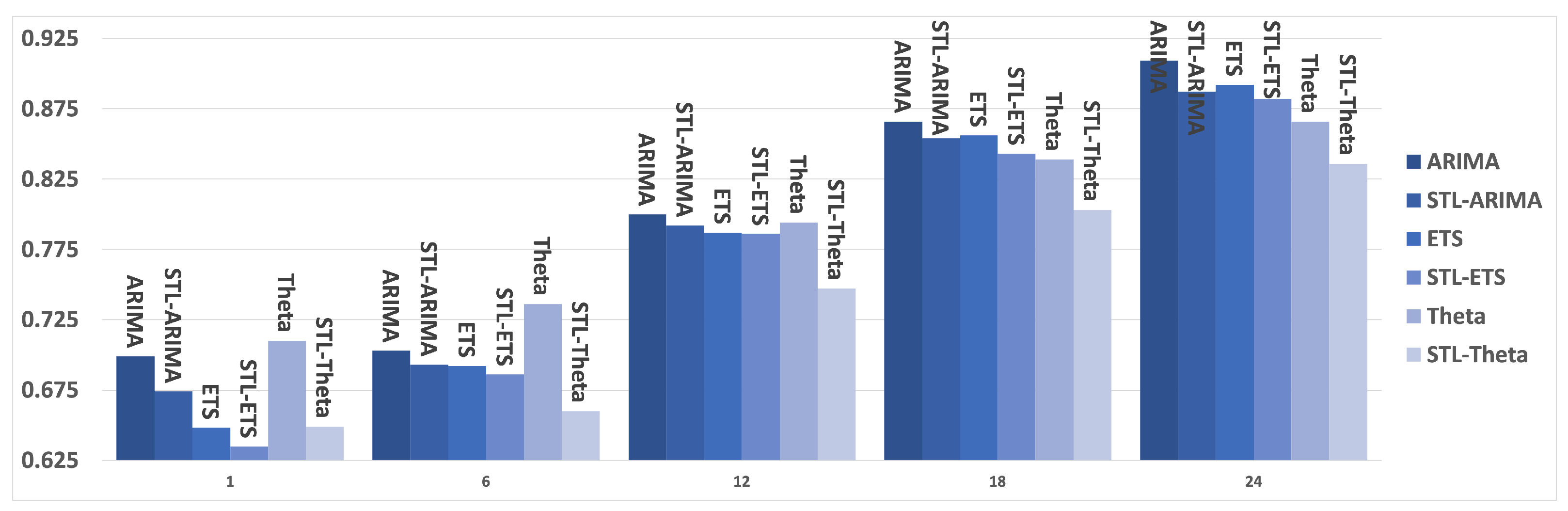
STL-ARIMA	8.245	0.604	0.674	9.915	0.717	0.693	11.755	0.856	0.792	13.457	0.993	0.854	14.481	1.093	0.887
STL-ETS	7.760	0.569	0.635	9.882	0.704	0.686	11.728	0.845	0.786	13.433	0.969	0.843	14.552	1.074	0.882
STL-Theta	7.963	0.580	0.649	9.502	0.678	0.660	11.177	0.801	0.747	12.817	0.921	0.803	13.891	1.011	0.836
ML & DL	h = 1			h = 6			h = 12			h = 18			h = 24
	sMAPE	MASE	OWA	sMAPE	MASE	OWA	sMAPE	MASE	OWA	sMAPE	MASE	OWA	sMAPE	MASE	OWA
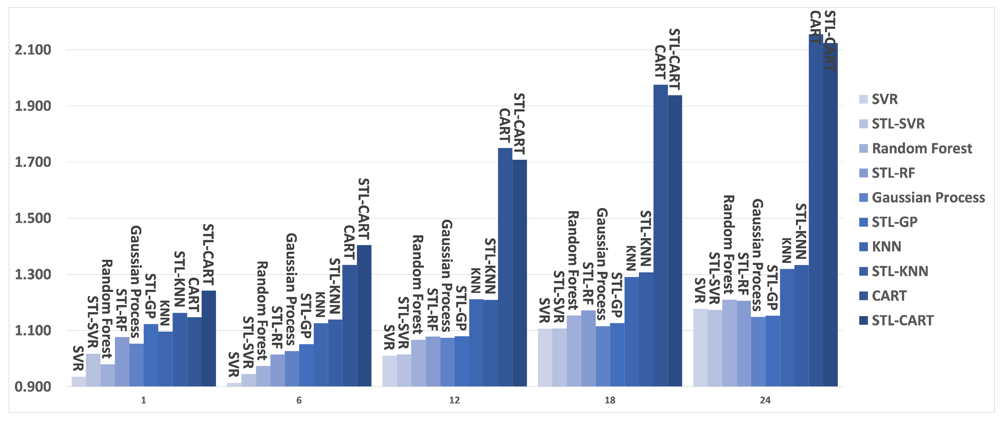
KNN	13.636	0.965	1.096	16.070	1.166	1.126	17.781	1.326	1.212	20.421	1.497	1.291	21.741	1.610	1.319
STL-KNN	15.318	1.077	1.228	18.359	1.390	1.313	17.980	1.306	1.210	22.513	1.698	1.444	22.154	1.610	1.332
SVR	11.253	0.855	0.936	12.732	0.971	0.914	14.712	1.116	1.011	17.485	1.284	1.107	19.526	1.429	1.178
STL-SVR	12.978	1.006	1.090	15.285	1.225	1.125	14.919	1.109	1.015	19.338	1.484	1.251	19.589	1.410	1.172
CART	14.080	1.025	1.147	19.081	1.377	1.334	25.490	1.930	1.750	30.934	2.314	1.975	35.956	2.596	2.155
STL-CART	15.820	1.191	1.310	21.715	1.660	1.561	25.157	1.862	1.708	32.285	2.446	2.075	35.715	2.537	2.124
RF	11.756	0.898	0.980	13.668	1.027	0.974	15.432	1.186	1.067	17.831	1.369	1.153	19.692	1.496	1.210
STL-RF	13.667	1.054	1.145	16.401	1.289	1.195	15.880	1.177	1.079	20.237	1.581	1.321	19.947	1.465	1.205
GP	12.540	0.972	1.053	14.268	1.093	1.027	15.528	1.195	1.075	17.395	1.313	1.116	18.720	1.418	1.148
STL-GP	14.163	1.120	1.201	16.950	1.351	1.244	15.782	1.187	1.080	19.624	1.526	1.278	18.974	1.408	1.152
CNN-LSTM	13.105	0.985	1.084	15.439	1.176	1.108	16.233	1.213	1.107	17.811	1.332	1.137	18.821	1.423	1.154
ConvLSTM	12.976	0.929	1.049	16.257	1.235	1.165	17.121	1.283	1.169	18.926	1.399	1.202	19.372	1.441	1.178

, Figure 1, Figure 2 and Figure 3, and the following contents.

Table 1 represents the forecast results of different methods on different forecast horizons. Note that Naïve 2 method was chosen as the reference method for the OWA indicator, meaning that OWA equals 1 whatever the horizon value h. At first glance, in Table 1, most of the statistical methods give better forecasting results with respect to naive methods (OWA < 1) than the machine learning methods (OWA > 1). This result confirms the conclusion from the M3 Competition that sophisticated machine learning methods do not assure a more accurate prediction than simple statistical methods.

This result becomes obvious in Figure 1, showing OWA ≤ 0.910 performance results for the three advanced statistical methods (ARIMA, ETS, and Theta), by comparison with Figure 2, showing OWA ≥ 0.914 performance results for the five machine learning methods. Above all, Figure 1 and Figure 2 show the impact of STL decomposition as a preprocessing step of statistical and ML methods on the forecasting performance results.

Significant improvement from STL decomposition was found for statistical methods. Among all the tested STL-based methods, the STL-Theta method outperforms the other methods on almost all forecast horizons. The STL-Theta method can even give a lower OWA on a 24-month forecast horizon than the other methods on the 18-month one.

In Figure 2, we can find that the SVR model gives the best result. No significant improvement from STL preprocessing was detected.

Figure 3 shows the mean and standard deviation of the gain brought by STL decomposition. On average, STL improves the OWA of ARIMA by 1.5%, ETS by 0.9%, and Theta by 5%, but it conducts a loss of OWA for machine learning methods. It harms SVR by 2.3%, RF by 3.3%, GP by 2.3%, KNN by 2.2%, and CART by 1.1%.

4.2. Discussion

It is interesting to note from the results in Figure 3 that CART performs the worst among all these methods, which is easy to understand as CART is a single forecaster. Its ensemble method Random Forest performs much better in terms of the precision of forecasting. At the same time, it consumes the most time.

The initial objective of this study was to determine whether STL decomposition can be helpful as a preprocessing step for time series forecasting methods. Our results confirm using STL decomposition as a preprocessing method can effectively improve the statistical methods’ performance, which is consistent with Theodosiou [23] using M1 Competition data, but, for machine learning methods, it can be harmful.

A possible explanation for this might be extracting the seasonal information from the series can affect the features to be modeled. For statistical models, their intrinsic ability for handling the seasonality might be worse than the STL decomposition. For the machine learning models, it could be easier to model seasonal data. Further research is required to confirm this hypothesis.

5. Conclusions

The present study was designed to determine the effect of using STL decomposition as a preprocessing step on different forecasting strategies. The results show some vast differences between these methods. Among all tested models, the STL decomposition-based Theta method is the best one. In the meantime, the STL decomposition can benefit the statistical methods by providing a more robust decomposition procedure than their intrinsic mechanism. The machine learning methods tested in this experimentation failed to outperform most statistical methods but still have some potentials for improvement. We can perform other preprocessing methods without harming the natural feature of the time series. More research is required in the future. For deep learning methods, as there are so many architectures and combinations of hyperparameters for neural networks, the two tested architectures in this experimentation may not be the optimal solutions. At the same time, there are many architectures more suitable for short sequence learning and worthy of further research.

References

- Zhang, G. Time series forecasting using a hybrid ARIMA and neural network model. Neurocomputing 2003, 50. [Google Scholar] [CrossRef]
- Box, G.E.P.; Jenkins, G.M.; Reinsel, G.C.; Ljung, G.M. Time Series Analysis: Forecasting and Control, 5th ed.; John Wiley & Sons, Inc.: Hoboken, NJ, USA, 2004; Volume 20. [Google Scholar]
- Kihoro, J.; Otieno, R.; Wafula, C. Seasonal time series forecasting: A comparative study of ARIMA and ANN models. Afr. J. Sci. Technol. 2004, 5. [Google Scholar] [CrossRef] [Green Version]
- Brown, R.G. Statistical Forecasting for Inventory Control; McGraw/Hill: New York, NY, USA, 1959. [Google Scholar]
- Holt, C.C. Forecasting seasonals and trends by exponentially weighted moving averages. Int. J. Forecast. 2004, 20. [Google Scholar] [CrossRef]
- Winters, P.R. Forecasting sales by exponentially weighted moving averages. Manag. Sci. 1960, 6, 324–342. [Google Scholar] [CrossRef]
- Hyndman, R.J.; Athanasopoulos, G. Forecasting: Principles and Practice; OTexts: Melbourne, Australia, 2018. [Google Scholar]
- Hyndman, R.J. A brief history of forecasting competitions. Int. J. Forecast. 2020, 36, 7–14. [Google Scholar] [CrossRef]
- Assimakopoulos, V.; Nikolopoulos, K. The theta model: A decomposition approach to forecasting. Int. J. Forecast. 2000, 16, 521–530. [Google Scholar] [CrossRef]
- Thomakos, D.D.; Nikolopoulos, K. Forecasting multivariate time series with the theta method. J. Forecast. 2015, 34, 220–229. [Google Scholar] [CrossRef] [Green Version]
- Hyndman, R.J.; Billah, B. Unmasking the Theta method. Int. J. Forecast. 2003, 19, 287–290. [Google Scholar] [CrossRef]
- Cleveland, R.B.; Cleveland, W.S.; McRae, J.E.; Terpenning, I. STL: A seasonal-trend decomposition. J. Off. Stat. 1990, 6, 3–73. [Google Scholar]
- Szegedy, C.; Toshev, A.; Erhan, D. Deep neural networks for object detection. In Proceedings of the 26th International Conference on Neural Information Processing Systems—Volume 2; Curran Associates Inc.: Red Hook, NY, USA, 2013. [Google Scholar]
- Graves, A. Supervised sequence labelling. In Supervised Sequence Labelling with Recurrent Neural Networks; Springer: Berlin/Heidelberg, Germany, 2012. [Google Scholar]
- Yurtsever, E.; Lambert, J.; Carballo, A.; Takeda, K. A survey of autonomous driving: Common practices and emerging technologies. IEEE Access 2020, 8. [Google Scholar] [CrossRef]
- Krizhevsky, A.; Sutskever, I.; Hinton, G.E. Imagenet classification with deep convolutional neural networks. In Proceedings of the 25th International Conference on Neural Information Processing Systems—Volume 1; Curran Associates Inc.: Red Hook, NY, USA, 2012. [Google Scholar]
- Sutskever, I.; Vinyals, O.; Le, Q.V. Sequence to sequence learning with neural networks. In Proceedings of the 27th International Conference on Neural Information Processing Systems—Volume 2; Curran Associates Inc.: Red Hook, NY, USA, 2014. [Google Scholar]
- Hinton, G.; Deng, L.; Yu, D.; Dahl, G.E.; Mohamed, A.R.; Jaitly, N.; Senior, A.; Vanhoucke, V.; Nguyen, P.; Sainath, T.N.; et al. Deep neural networks for acoustic modeling in speech recognition: The shared views of four research groups. IEEE Signal Process. Mag. 2012, 29, 82–97. [Google Scholar] [CrossRef]
- Lapedes, A.; Farber, R. Nonlinear Signal Processing Using Neural Networks: Prediction and System Modelling; Technical Report (No. LA-UR-87-2662; CONF-8706130-4); Los Alamos National Laboratory: Los Alamos, NM, USA, 1987. [Google Scholar]
- Hastie, T.; Tibshirani, R.; Friedman, J. The Elements of Statistical Learning: Data Mining, Inference, and Prediction; Springer Science & Business Media: Berlin/Heidelberg, Germany, 2009. [Google Scholar]
- Ahmed, N.K.; Atiya, A.F.; Gayar, N.E.; El-Shishiny, H. An empirical comparison of machine learning models for time series forecasting. Econom. Rev. 2010, 29. [Google Scholar] [CrossRef]
- Makridakis, S.; Spiliotis, E.; Assimakopoulos, V. Statistical and Machine Learning forecasting methods: Concerns and ways forward. PLoS ONE 2018, 13, e0194889. [Google Scholar] [CrossRef] [Green Version]
- Theodosiou, M. Forecasting monthly and quarterly time series using STL decomposition. Int. J. Forecast. 2011, 27, 1178–1195. [Google Scholar] [CrossRef]
- Makridakis, S.; Spiliotis, E.; Assimakopoulos, V. The M4 Competition: 100,000 time series and 61 forecasting methods. Int. J. Forecast. 2020, 36, 54–74. [Google Scholar] [CrossRef]
- Bontempi, G.; Taieb, S.B.; Le Borgne, Y.A. Machine learning strategies for time series forecasting. In European Business Intelligence Summer School; Springer: Berlin/Heidelberg, Germany, 2012. [Google Scholar]
- Breiman, L. Random forests. Mach. Learn. 2001, 45, 5–32. [Google Scholar] [CrossRef] [Green Version]
- Rasmussen, C.E. Gaussian processes in machine learning. In Summer School on Machine Learning; Springer: Berlin/Heidelberg, Germany, 2003. [Google Scholar]
- Shi, X.; Chen, Z.; Wang, H.; Yeung, D.Y.; Wong, W.K.; Woo, W.C. Convolutional LSTM network: A machine learning approach for precipitation nowcasting. In Proceedings of the 28th International Conference on Neural Information Processing Systems—Volume 1; Curran Associates Inc.: Red Hook, NY, USA, 2015. [Google Scholar]
- Hochreiter, S.; Schmidhuber, J. Long short-term memory. Neural Comput. 1997, 9, 1735–1780. [Google Scholar] [CrossRef] [PubMed]
- R Core Team. R: A Language and Environment for Statistical Computing; R Foundation for Statistical Computing: Vienna, Austria, 2020. [Google Scholar]
- Hyndman, R.J.; Khandakar, Y. Automatic time series forecasting: The forecast package for R. J. Stat. Softw. 2008, 27. [Google Scholar] [CrossRef] [Green Version]
- Seabold, S.; Perktold, J. Statsmodels: Econometric and statistical modeling with python. In Proceedings of the 9th Python in Science Conference (SciPy 2010), Austin, TX, USA, 28 June–3 July 2010. [Google Scholar]
- Pedregosa, F.; Varoquaux, G.; Gramfort, A.; Michel, V.; Thirion, B.; Grisel, O.; Blondel, M.; Prettenhofer, P.; Weiss, R.; Dubourg, V.; et al. Scikit-learn: Machine learning in Python. J. Mach. Learn. Res. 2011, 12, 2825–2830. [Google Scholar]
- Löning, M.; Bagnall, A.; Ganesh, S.; Kazakov, V.; Lines, J.; Király, F.J. sktime: A unified interface for machine learning with time series. arXiv 2019, arXiv:1909.07872. [Google Scholar]
- Chollet, F. Keras. 2015. Available online: https://keras.io (accessed on 13 October 2020).
- Abadi, M.; Agarwal, A.; Barham, P.; Brevdo, E.; Chen, Z.; Citro, C.; Corrado, G.S.; Davis, A.; Dean, J.; Devin, M.; et al. TensorFlow: Large-Scale Machine Learning on Heterogeneous Systems. 2015. Available online: tensorflow.org (accessed on 13 October 2020).
- Makridakis, S. Accuracy measures: Theoretical and practical concerns. Int. J. Forecast. 1993, 9, 527–529. [Google Scholar] [CrossRef]
- Hyndman, R.J.; Koehler, A.B. Another look at measures of forecast accuracy. Int. J. Forecast. 2006, 22, 679–688. [Google Scholar] [CrossRef] [Green Version]