Flow and Density Estimation in Grenoble Using Real Data ^†

Abstract

This work deals with the Traffic State Estimation (TSE) problem for urban networks, using heterogeneous sources of data such as stationary flow sensors, Floating Car Data (FCD), and Automatic Vehicle Identifiers (AVI). A data-based flow and density estimation method is presented and tested using real traffic data. This work presents a study case applied to the downtown of the city of Grenoble in France, using the Grenoble Traffic Lab for urban networks (GTL-Ville), which is an experimental platform for real-time collection and analysis of traffic data.

1. Introduction

Traffic state estimation (TSE) is an important stage in the development of Intelligent Transportation Systems (ITS), as the knowledge of the evolution of traffic state variables such as flow and density for each road can be used to implement control strategies, or help in the decision-making stages for network design for better smart cities. TSE refers to the use of partially observed and noisy traffic data to infer the value of traffic indicators such as flow, density, velocity, traveling time, and others [1]. This information can be used to calculate the mean traveling times for users, fuel consumption and vehicle emissions (important for air quality assessment), estimate the life of pavement, and many other applications. Because of this, accurate TSE is an active field in the transportation research literature [2].

Classical TSE methods were initially proposed for the case of highways [3]. Generally, these methods are based on the Lighthill–Whitham [4] and Richards [5] (LWR) model, and its discrete counterpart, the Cell Transmission Model (CTM) [6], which use the empirical flow-density relation known as the Fundamental Diagram. In [7], the authors propose the use of an Extended Kalman Filter (EKF) by linearizing the CTM around a current state to estimate the density of road sections. In [8], the CTM is used to identify observable modes, where a graph-constrained density observer is applied. In [9], semi-analytical solutions to the LWR are coupled with a mixed integer problem to estimate highway density.

The case of networks has received less attention [2], but the need to study this scenario is increasing in the last few years for TSE issues. This relative lack of attention is due to the additional modeling tools required to describe vehicle interactions in intersections [10]. The extended version of the CTM developed in [11] brings a solution to this problem via a flow maximization formulation under constraints provided by the fundamental diagram. This approach is widely used as can be seen in [12,13]. However, the use of the fundamental diagram, especially in urban networks, is challenging as it requires the calibration of many parameters. Furthermore, recent studies have found that the fundamental diagram does not effectively describe vehicle deceleration at intersections [14]. To solve this issue, the authors in [15] proposed a data-based method that collects data from connected vehicles to estimate the exiting flow of each road. Nevertheless, such rich data are not always available, and other methods are required.

Our contribution in this paper is the proposal of a data-based TSE method for general urban networks. We make use of three different data sources: stationary flow sensors, AVI using Bluetooth devices, and Floating Car Data (FCD). Data provided by these sources are used to estimate the external inflows to a traffic network, the turning ratios for a selection of intersections, and the space mean speed of the road sections of the network. Additionally, the method is tested using real traffic data collected from a sensor network in the city of Grenoble, France.

This paper is organized as follows. Section 2 presents the traffic dynamics model used to estimate the flow and density for the road sections of an urban traffic network. Section 3 describes the experimental platform Grenoble Traffic Lab (GTL-Ville), and the available data used to deploy and validate the proposed model. Section 4 describes a method used to estimate some of the parameters of the model that are not measured directly. Section 5 presents the results of the estimation approach and compares them to real data. Finally, Section 6 ends the paper with some conclusions.

2. Density Estimation Model

We consider urban traffic networks which are modeled as a directed graph $\mathcal{G}=\{\mathcal{N},\mathcal{E}\}$ where the nodes $\mathcal{N}$ correspond to intersections, and the edges $\mathcal{E}\subset \mathcal{N}\times \mathcal{N}$ correspond to road sections. Additionally, let ${\mathcal{E}}^{\mathrm{in}}\subset \mathcal{E}$ denote the boundary incoming roads which have no upstream neighbors, and ${\mathcal{E}}^{\mathrm{out}}\subset \mathcal{E}$ denote the boundary outgoing roads that have no downstream neighbors.

For all roads, we consider as state variables the density $\mathbf{\rho }$ (veh/km), incoming flow ${\mathbf{\phi }}^{\mathrm{in}}$ (veh/h), outgoing flow ${\mathbf{\phi }}^{\mathrm{out}}$ (veh/h), and space–mean velocity $\mathbf{v}$ (km/h), which are all time dependent and have dimensions equal to the number of roads $\left|\mathcal{E}\right|$.

To model the traffic dynamics, consider the following conservation law for the traffic density [16],

$$\frac{\mathrm{d}}{\mathrm{d}t}\mathbf{\rho }\left(t\right)=L^{-1}({\mathbf{\phi }}^{\mathrm{in}}\left(t\right)-{\mathbf{\phi }}^{\mathrm{out}}\left(t\right))$$

(1)

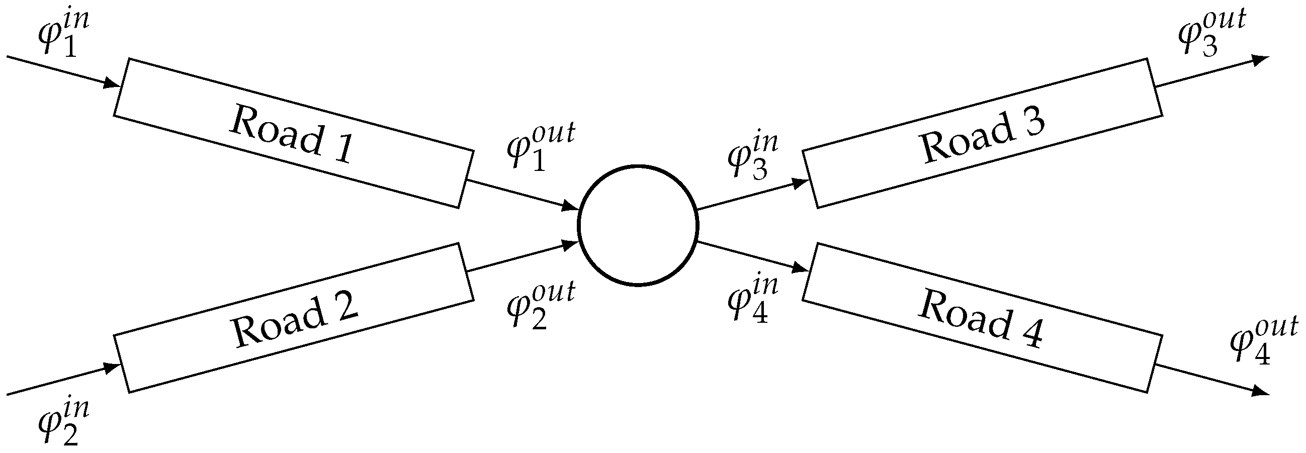
where L is a diagonal matrix containing the road lengths. Furthermore, the inflows and outflows of adjacent roads are dependent on each other through intersections as shown in Figure 1. Intersections are modeled as 0-dimensional points that do not store vehicles. To model the exchange of inflows and outflows of the different roads at the intersections, we use the parameters called turning ratios. Let $\mathcal{I}\left(n\right)$ be the set of incoming roads to some intersection $n\in \mathcal{N}$ and $\mathcal{O}\left(n\right)$ be the set of outgoing roads from n. A turning ratio $r_{i,j}$ for $i\in \mathcal{I}\left(n\right)$ and $j\in \mathcal{O}\left(n\right)$ defines the proportion of vehicles exiting i that enters j.

As intersections do not store vehicles, then the conservation of density implies that

$$\sum _{j\in \mathcal{O}\left(n\right)}{r}_{i,j}=1,\forall n\in \mathcal{N}\forall i\in \mathcal{E}\setminus {\mathcal{E}}^{\mathrm{out}}.$$

(2)

Let $R\in {\mathbb{R}}^{\left|\mathcal{E}\right|\times \left|\mathcal{E}\right|}$ be the turning ratio matrix with elements $r_{i,j}$. If there is no connection between roads $i,j$, then $R_{i,j}=0$. The input flows of each section can be expressed as a linear combination of the output flows of the preceding sections:

$${\mathbf{\phi }}^{\mathrm{in}}\left(t\right)=R^{\top }{\mathbf{\phi }}^{\mathrm{out}}\left(t\right)+B\mathbf{u}\left(t\right)$$

(3)

where $\mathbf{u}\left(t\right)$ is the vector of input demands at the boundaries of the network, and B is a selection matrix which identifies the elements of ${\mathcal{E}}^{\mathrm{in}}$. Combining Equations (1) and (3), we have

$$\frac{\mathrm{d}}{\mathrm{d}t}\mathbf{\rho }\left(t\right)=L^{-1}(R^{\top }-\mathbb{I}){\mathbf{\phi }}^{\mathrm{out}}\left(t\right)+L^{-1}B\mathbf{u}\left(t\right)$$

(4)

Using the hydrodynamic relation, we can approximate the outflows of each road from the values of density and the space–mean speed as

$${\mathbf{\phi }}^{\mathrm{out}}\left(t\right)\approx V\left(t\right)\mathbf{\rho }\left(t\right)$$

(5)

where $V\left(t\right)=\mathrm{diag}\left(\mathbf{v}\right(t\left)\right)$. This relation applies accurately when considering very short distances, or when the spatial variations in vehicle speed and density are negligible. We make the following assumption:

Assumption 1.

The speed and density throughout a road section do not vary significantly in the spatial domain.

In urban settings, this assumption can be justified as road lengths between intersections are generally on the order of 100 m. Therefore, we rewrite (4) as

$$\frac{\mathrm{d}}{\mathrm{d}t}\mathbf{\rho }\left(t\right)=L^{-1}(R^{\top }-\mathbb{I})V\left(t\right)\mathbf{\rho }\left(t\right)+L^{-1}B\mathbf{u}\left(t\right)$$

(6)

In this work, we consider the use of (6) as an open-loop estimator for the state of the network. To achieve this goal, we require as input data the values of the turning ratios for all intersections, the space–mean road speeds, and the input demands. Denote by $\widehat{R}$, $\widehat{V}$ and $\widehat{\mathbf{u}}$ the estimated or measured values for these variables. Thus, the proposed density estimator is

$$\frac{\mathrm{d}}{\mathrm{d}t}\widehat{\mathbf{\rho }}\left(t\right)=L^{-1}({\widehat{R}}^{\top }-\mathbb{I})\widehat{V}\left(t\right)\widehat{\mathbf{\rho }}\left(t\right)+L^{-1}\widehat{\mathbf{u}}\left(t\right)$$

(7)

In the next section, we describe how the estimated quantities for the input data are obtained.

3. Experimental Platform

In this work, we make use of the Grenoble Traffic Lab for Urban Networks, GTL-Ville (http://gtlville.inrialpes.fr, accessed on 29 June 2021). This is an experimental platform for real-time collection of traffic data coming from a network of sensors installed in the city of Grenoble, France. This platform also provides real-time traffic indicators and analysis oriented towards the users of the city, traffic operators, and researchers. The collected data and computed indicators are available for download at the website.

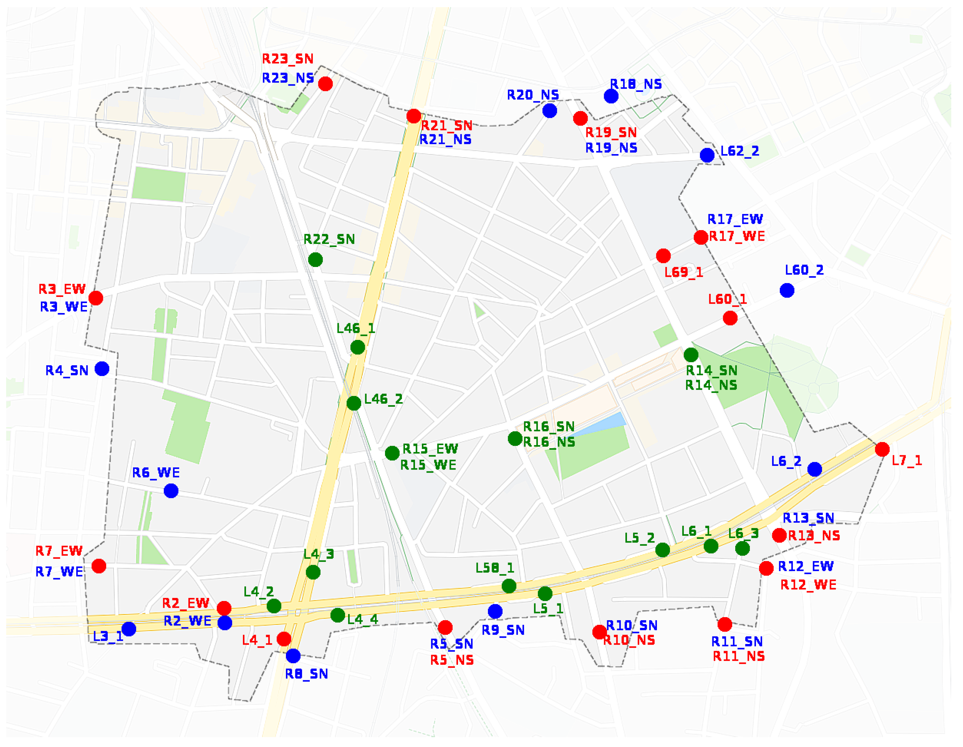
In this work, we consider a section of Grenoble’s downtown of an area of approximately 1.4 km by 1 km (see Figure 2). In this section, we describe the available data for the intersections and roads contained in this section.

3.1. Stationary Counting Sensors

Stationary sensors are placed in a fixed position in a road section, and collect information of the vehicles passing through that point. The collected data vary according to the technology, but generally variables such as length, speed, and time of passage are recorded. Two sensor technologies are available:

• Induction loop sensors, installed under the pavement, detect changes in the inductance due to the passage of vehicles. It provides information about flow and occupancy.
• Microwave radars, located above the ground, emit pulses of radiation and then measure the properties of the reflected beam. It provides information about flow, vehicle speeds, and length.

The sensor locations are shown in Figure 2. Induction loop sensors have an identifier starting with “L”, whereas microwave radars start with “R”. Each dot corresponds to the location of a single sensor. As radars are able to measure in multiple lanes and directions, some locations present two identifiers that correspond to each direction.

Furthermore, according to their locations, sensor data are classified as

• Boundary inflows (blue dots in the figure), providing the values of $\widehat{\mathbf{u}}\left(t\right)$ in Equation (7).
• Boundary outflows (red dots in the figure). Data from these locations are denoted by $\mathbf{y}\left(t\right)$.
• Validation flows (green dots in the figure). Data from these locations will be used to validate estimation results.

3.2. Floating Car Data

Floating Car Data (FCD) are trajectories of individual vehicles collected via devices such as GPS navigators. Due to privacy policies, data from multiple users are aggregated.

Define by ${\mathcal{V}}_i\left(t\right)$ the set of vehicle indexes that provide FCD that are inside road i at time t. Let ${\nu }_{\alpha }$ be the speed of a vehicle indexed by $\alpha$. We define the aggregated speed for road section i from FCD data by

$${\widehat{v}}_i\left(t\right)=\frac{1}{|{\mathcal{V}}_i\left(\tau \right)|}\sum _{\alpha \in {\mathcal{V}}_i\left(t\right)}{\nu }_{\alpha }\left(t\right)$$

(8)

which provides the estimates of the space–mean speeds for all roads, $\widehat{V}\left(t\right)$ in Equation (7). However, this information is not available for roads that have few vehicles during the day, resulting in low precision estimates. For this cases, we use the value of the free-flow velocity, as roads with few vehicles are often under the critical density.

3.3. Turning Ratio Measurements

To measure the values of the turning ratio parameters, Bluetooth vehicle identifiers were used. For a given intersection, these devices are located at the adjacent incoming and outgoing roads. During a time interval, each device is able to detect vehicles that are equipped with another Bluetooth device, and records a unique identifier and its time of passage. By comparing the information across the installed devices, it is possible to assign the origin and destination road of individual vehicles.

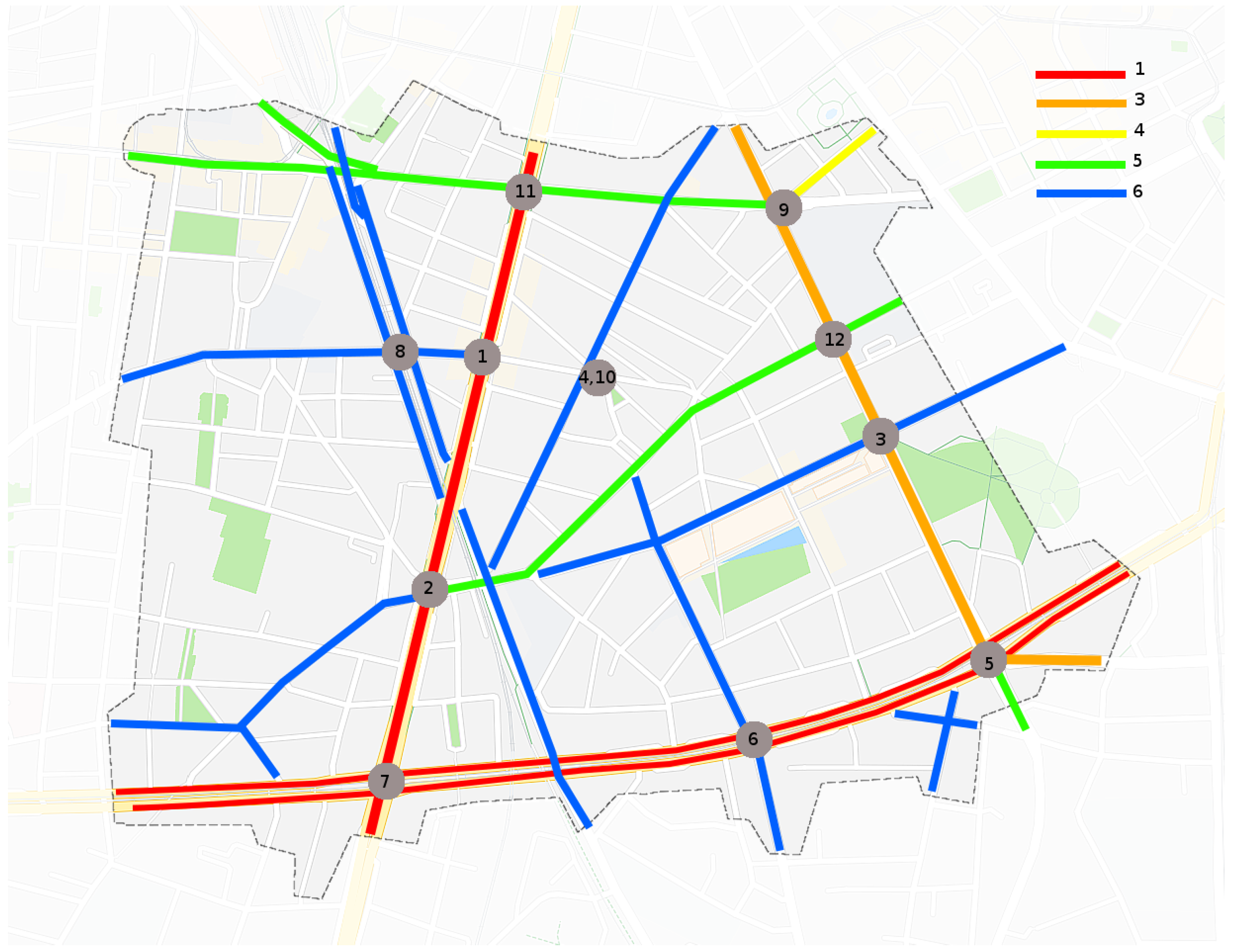
As the rate of vehicles equipped with Bluetooth devices is unknown, these measurements cannot provide the total flow. However, this information can be used to compute the relative use of each turn, so the turning ratios can be estimated. Due to economical constraints, only 12 intersections were monitored during a measurement campaign lasting one week. Denote by $\mathcal{B}\subset \mathcal{N}$ the set of intersection monitored by these devices, whose locations are shown in Figure 3. The corresponding turning ratios are computed as

$$r_{i,j}^{\mathrm{BT}}=\frac{\mathrm{Counts}(i,j)}{{\sum }_k\mathrm{Counts}(i,k)}$$

(9)

where $\mathrm{Counts}(i,j)$ is the total number of detected vehicles going from road i to j during the campaign duration. To provide turning ratio estimates for the remaining intersections, a method is described in Section 4 which uses the data presented in Section 3.4.

3.4. Functional Road Classification

The Functional Road Classification (FRC) is used to classify roads into homogeneous classes depending on their role in a transportation network [17]. This classification determines the type of use of each road, for instance, as it differentiates between major roads that experience heavy traffic from a variety of O/D pairs, and minor roads which are inside of a residential area and experience light traffic only. Figure 3 shows the FRC of each road of the considered zone of Grenoble, and

Table 1. Description of the road classes provided by TomTom.

Class	Short Description	Long Description
1	Major roads of high importance	Roads of high importance that are used for international and national traffic.
2	Other major roads	Roads used to travel between neighboring country regions.
3	Secondary roads	Roads used to travel between parts of the same region.
4	Local connecting roads	Roads making settlements accessible or making parts of a settlement accessible.
5	Local roads of high importance	Local roads that are the main connections in a settlement.
6	Local roads	Roads used to travel within a part of a settlement.
7	Local roads of minor importance	Roads that only have a destination function.

shows each class description (Source: https://developer.tomtom.com/traffic-stats/support/faq/what-are-functional-road-classes-frc, accessed on 29 June 2021). Roads that are not colored in the figure have class 7.

4. Parameter Estimation

To estimate the values of the turning ratio parameters for the intersections that have no direct measurement (see Section 3.3), we propose the use of the FRC information. The reasoning for this is that roads with a higher importance are more commonly used than smaller roads, and will therefore present higher turning ratios.

For each FRC class in the set $\{1,2,\cdots ,7\}$, we define a weight $\theta \in (0,1]$. Let $\mathbf{\theta }\in {(0,1]}^7$ be the vector of class weights. Suppose that the turning ratios at each intersection are distributed proportionally to the class weights of each of its outgoing roads. Thus, these parameters are computed as

$$r_{i,j}^{\mathrm{FRC}}=\frac{{\theta }_{\mathrm{FRC}\left(j\right)}}{{\displaystyle \sum _{k\in \mathcal{O}\left(n_i\right)}{\theta }_{\mathrm{FRC}\left(k\right)}}}$$

(10)

where $\mathrm{FRC}\left(i\right)$ is the FRC class of road i, $n_i$ is the intersection connected to i, and $\mathcal{O}\left(n_i\right)$ is the set of outgoing roads from intersection $n_i$.

To compute the value of $\mathbf{\theta }$, we consider the following optimization problem:

$$\begin{array}{cc}\hfill \underset{\mathbf{\theta }}{\min }& \left|\right|\overline{\mathbf{y}}-C{(\mathbb{I}-{\widehat{R}}^{\top }\left(\mathbf{\theta }\right))}^{-1}B\overline{\mathbf{u}}\left|\right|\hfill \\ \\ \hfill \mathrm{subject}\mathrm{to}& \mathbf{\theta }\in {(0,1]}^7,\hfill \\ \hfill & {\theta }_1=1,\hfill \\ \hfill & {\widehat{R}}_{i,j}\left(\mathbf{\theta }\right)=\left\{\begin{array}{ccc}{r}_{i,j}^{\mathrm{BT}}& \mathrm{if}& n_i\in \mathcal{B}\\ \\ r_{i,j}^{\mathrm{FRC}}& \mathrm{if}& n_i\notin \mathcal{B}\end{array}\right.\hfill \end{array}$$

(11)

where C is a selection matrix which identifies the outgoing roads ${\mathcal{E}}^{\mathrm{out}}$, and

$$\overline{\mathbf{u}}=\frac{1}{T}{\int }_0^T\mathbf{u}\left(t\right),\overline{\mathbf{y}}=\frac{1}{T}{\int }_0^T\mathbf{y}\left(t\right).$$

(12)

are the average flows from the input and output sets, respectively. This optimization problem tries to match the observed outflows of the network with the outflows computed from the measured inflows and the turning ratio estimates,

$$\widehat{\mathbf{y}}=C{(\mathbb{I}-{\widehat{R}}^{\top })}^{-1}B\overline{\mathbf{u}}.$$

(13)

The condition ${\theta }_1=1$ is set arbitrarily without loss of generality, as only the relative differences between the weights are important.

Due to the limited number of parameters, this problem can be solved with common optimization solvers. We obtained the values shown in

Table 2. Value of FRC weights for the estimation of turning ratio parameters.

Class index	1	2	3	4	5	6	7
Class weight $\theta$	1.00	N/A	1.00	0.50	0.23	0.13	0.03

(The considered network has no road with FRC 2. Thus, its weight does not affect the calculations). Note that, as the importance of the road decreases, so does the corresponding class weight as is to be expected.

5. Experimental Results

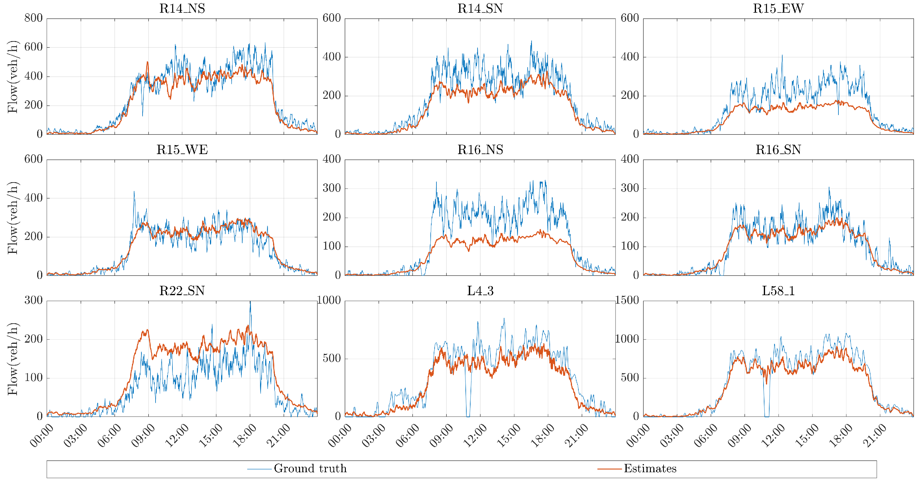
For evaluation purposes, we considered the data collected for 8 January 2021. Figure 4 shows the time series for the real and estimated flows for a selection of validation sensors. Note that, for most cases, the estimated and real values have a very similar trajectory. The mismatches obtained for some of the sensors can be attributed to several factors. The main source of error is due to deviations between the real and estimated turning ratios. As these parameters were computed using a simplifying hypothesis using the FRC, there are intersections for which the obtained values present error. However, this method provides a simple to use manner to compute these parameters for large networks with easily obtainable information, and provides good initial results for a large number of locations which can be improved with time. Another possible error source is the presence of internal sources and sinks of traffic flow which are not taken into account.

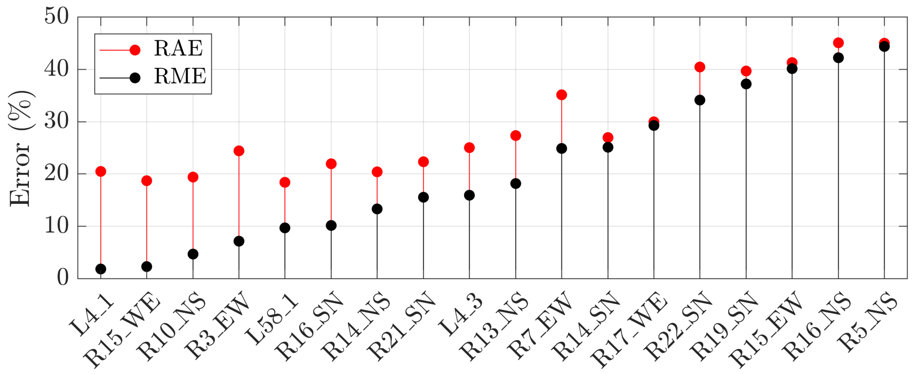
To quantify the error in time for each location, we use as error metrics the Relative Mean Error (RME) and the Relative Absolute Error (RAE), defined as

$$\begin{array}{ccc}{\mathrm{RME}}_i=\frac{\left|{\displaystyle {\int }_0^T{\phi }_i^{\mathrm{out}}\left(t\right)-{\widehat{\phi }}_i^{\mathrm{out}}\left(t\right)\mathrm{d}t}\right|}{{\displaystyle {\int }_0^T{\phi }_i^{\mathrm{out}}\left(t\right)\mathrm{d}t}}& ,& {\mathrm{RAE}}_i=\frac{{\displaystyle {\int }_0^T\left|{\phi }_i^{\mathrm{out}}\left(t\right)-{\widehat{\phi }}_i^{\mathrm{out}}\left(t\right)\right|\mathrm{d}t}}{{\displaystyle {\int }_0^T{\phi }_i^{\mathrm{out}}\left(t\right)\mathrm{d}t}}\end{array}.$$

(14)

Figure 5 shows the obtained error metrics for all the available validation sensors. The RME shows that the proposed estimator provides close estimates to the real values, as half of the validation locations present an error under 20%, and all cases presented an error under 50%. When considering the RAE, the error increases as this metric considers not only the differences between the mean trajectories, but also takes into account the dispersion of the real data. Nevertheless, for half of the locations, the RAE lies between 20% and 30% showing a good agreement of the estimation with the real data. Similarly to the RME, all locations have a RAE under 50%.

6. Conclusions

In this paper, we proposed a data-based flow and density estimator that uses heterogeneous data sources such as stationary counting sensors, FCD, and Bluetooth devices. The estimator was tested using real data from the city of Grenoble, France, using the sensing infrastructure developed in the project GTL-Ville.

Although the problem of TSE in large networks is challenging, the obtained results are encouraging as the estimated flow for individual roads are very close to the ground truth data provided by sensors. When considering all the available validation locations, more than half of the mean trajectories presented an error below 20%. For some locations, there is a mismatch between the predicted flow and the real one. Nevertheless, even in this case, the obtained errors were below 45%. We identify as the main error source the uncertainty in the values of the turning ratios, as only a few locations are computed using real data. However, this can be improved in the future by performing more measuring campaigns, so the estimation results in the real application are expected to improve significantly.

References

- Treiber, M.; Kesting, A. Traffic Flow Dynamics: Data, Models and Simulation; Springer: Berlin/Heidelberg, Germany, 2013; pp. 1–503. [Google Scholar]
- Seo, T.; Bayen, A.M.; Kusakabe, T.; Asakura, Y. Traffic state estimation on highway: A comprehensive survey. Annu. Rev. Control. 2017, 43, 128–151. [Google Scholar] [CrossRef] [Green Version]
- Ferrara, A.; Sacone, S.; Siri, S. Freeway Traffic Modelling and Control, 1st ed.; Advances in Industrial Control; Springer International Publishing: Cham, Switzerland, 2018. [Google Scholar]
- Lighthill, M.J.; Whitham, G.B. On kinematic waves II. A theory of traffic flow on long crowded roads. Proc. R. Soc. London. Ser. A Math. Phys. Sci. 1955, 229, 317–345. [Google Scholar]
- Richards, P.I. Shock Waves on the Highway. Oper. Res. 1956, 4, 42–51. [Google Scholar] [CrossRef]
- Daganzo, C.F. The cell transmission model: A dynamic representation of highway traffic consistent with the hydrodynamic theory. Transp. Res. Part B 1994, 28, 269–287. [Google Scholar] [CrossRef]
- Tampère, C.M.; Immers, L.H. An extended Kalman filter application for traffic state estimation using CTM with implicit mode switching and dynamic parameters. In Proceedings of the 2007 IEEE Intelligent Transportation Systems Conference, Seattle, WA, USA, 30 September–3 October 2007; pp. 209–216. [Google Scholar]
- Canudas-de Wit, C.; Ojeda, L.L.; Kibangou, A.Y. Graph constrained-CTM observer design for the Grenoble south ring. FAC Proc. Vol. 2012, 45, 197–202. [Google Scholar] [CrossRef] [Green Version]
- Canepa, E.S.; Claudel, C.G. Networked traffic state estimation involving mixed fixed-mobile sensor data using Hamilton-Jacobi equations. Transp. Res. Part B Methodol. 2017, 104, 686–709. [Google Scholar] [CrossRef] [Green Version]
- Jabari, S.E. Node modeling for congested urban road networks. Transp. Res. Part B Methodol. 2016, 91, 229–249. [Google Scholar] [CrossRef]
- Daganzo, C.F. The cell transmission model, part II: Network traffic. Transp. Res. Part B 1995, 29, 79–93. [Google Scholar] [CrossRef]
- Lovisari, E.; Canudas-de Wit, C.; Kibangou, A.Y. Density/Flow reconstruction via heterogeneous sources and Optimal Sensor Placement in road networks. Transp. Res. Part C Emerg. Technol. 2016, 69, 451–476. [Google Scholar] [CrossRef] [Green Version]
- Ladino, A.; Canudas-de Wit, C.; Kibangou, A.; Fourati, H.; Rodriguez, M. Density and flow reconstruction in urban traffic networks using heterogeneous data sources. In Proceedings of the 2018 European Control Conference (ECC), Limassol, Cyprus, 12–15 June 2018; pp. 1679–1684. [Google Scholar]
- Liou, H.T.; Hu, S.R.; Peeta, S. Estimation of Time-Dependent Intersection Turning Proportions for Adaptive Traffic Signal Control under Limited Link Traffic Counts from Heterogeneous Sensors; Technical Report; NEXTRANS Center, Purdue University: West Lafayette, IN, USA, 2017. [Google Scholar]
- Rostami Shahrbabaki, M.; Safavi, A.A.; Papageorgiou, M.; Setoodeh, P.; Papamichail, I. State estimation in urban traffic networks: A two-layer approach. Transp. Res. Part C Emerg. Technol. 2020, 115, 102616. [Google Scholar] [CrossRef]
- Bianchin, G.; Pasqualetti, F.; Kundu, S. Resilience of Traffic Networks with Partially Controlled Routing. In Proceedings of the 2019 American Control Conference (ACC), Philadelphia, PA, USA, 10–12 July 2019; pp. 2670–2675. [Google Scholar]
- D’Andrea, A.; Cappadona, C.; La Rosa, G.; Pellegrino, O. A functional road classification with data mining techniques. Transport 2014, 29, 419–430. [Google Scholar] [CrossRef] [Green Version]
Figure 1.
Flow exchange at an intersection.
Figure 2.
Stationary flow sensors located in downtown Grenoble. The text refers to sensor identifiers. Sensors in blue, correspond to boundary inflows; in red to boundary outflows; and in green to validation flows.
Figure 3.
Grey dots: intersections equipped with Bluetooth identifier devices. Colored lines: functional road classification of the network.
Figure 4.
Ground truth flows obtained from cross-validation sensors, and the corresponding estimated flows.
Figure 5.
RME and RAE obtained for the available validation and output sensors.