
Predictability of Scrub Typhus Incidences Time Series in Thailand †

1
Solidarity, Societies, Territories, Interdisciplinary Laboratory LISST UMR 5193, CNRS—University of Toulouse Jean-Jaurès, 31000 Toulouse, France
2
Strathclyde Centre for Environmental Law and Governance (SCELG), University of Strathclyde, Glasgow G11, UK
3
INSERM, Laboratory Population Environment Development, IRD UMR 151, Aix Marseille University, IRD, 13331 Marseille, France
*
Author to whom correspondence should be addressed.
†
Presented at the 7th International conference on Time Series and Forecasting, Gran Canaria, Spain, 19–21 July 2021.
Eng. Proc. 2021, 5(1), 44; https://0-doi-org.brum.beds.ac.uk/10.3390/engproc2021005044
Published: 13 July 2021
(This article belongs to the Proceedings of The 7th International Conference on Time Series and Forecasting)
Abstract
:Scrub typhus, an infectious disease caused by a bacterium transmitted by “chigger” mites, constitutes a public health problem in Thailand. Predicting epidemic peaks would allow implementing preventive measures locally. This study analyses the predictability of the time series of incidence of scrub typhus aggregated at the provincial level. After stationarizing the time series, the evaluation of the Hurst exponents indicates the provinces where the epidemiological dynamics present a long memory and are predictable. The predictive performances of ARIMA (autoregressive integrated moving average model), ARFIMA (autoregressive fractionally integrated moving average) and fractional Brownian motion models are evaluated. The results constitute the reference level for the predictability of the incidence data of this zoonosis.
Keywords:
infectious disease; predictability; incidence; time series; ARIMA; ARFIMA; fBm; scrub typhus; Thailand1. Introduction
Scrub typhus is a relatively underdiagnosed infectious disease, affecting approximately 1 million people worldwide. It is caused by Orientia tsutsugamushi, a bacterium transmitted by “chigger” mites that mostly parasitize rodents, humans being only accidentally a host. In the Mekong region of Southeast Asia, the frequency of isolation of pathogens implicated in the aetiology of non-malarial febrile illness has shown that Orientia tsutsugamushi was, immediately following dengue virus, the most frequently reported [1,2]. In Thailand, the sporadic incidence in humans reported by the Armed Forces Research Institute of Medical Sciences for 2018 and 2019, respectively, was 7.11 and 5.82 individuals per 100,000 populations [3]. Although scrub typhus is endemic in various countries of Asia and Southeast Asia [4], it remains an underdiagnosed disease and its public health burden is still poorly known [5]. While knowing the distribution and the factors that may contribute to the disease incidence is essential for public health [6], it is also crucial to understand the seasonal trend of scrub typhus in order to be ready to adopt the appropriate public health response. Indeed, the study of time series of incidence of scrub typhus aggregated at the provincial level may help to forecast future incidence [7], to monitor the evolution of the trend of the diseases and thus to prevent and control the outbreaks of the disease by providing a way to facilitate decision-making and determine whether an apparent excess represents an outbreak rather than a random variation [8].
Anticipating the timing and severity of the peak can improve the decision-making in real time [9,10] and help allocating the resources needed during public health emergencies [11]. The analysis of the predictability of the time series of incidence of scrub typhus also presents a double interest from the point of view of the knowledge of this infectious disease and its modelling: (a) it involves evaluating a property intrinsic to its epidemiological dynamics (the long-term dependence of the number of cases being likely to vary significantly from one province to another.); (b) it offers a decisive criterion for testing the performance of the models and their usefulness for prevention. After presenting the data from the Thai Ministry of Public Health and their aggregation in Section 2, the predictive models used are briefly presented in Section 3 as well as the criteria used for their evaluation. The results concerning the predictability of scrub typhus time series are gathered and discussed in Section 4, before concluding in Section 5.
2. Data Time Series of Scrub Typhus Incidences
The analyzed data are provided by the Thai Ministry of Public Health. More than 110,000 individual cases have been diagnosed in Thailand between January 2003 and December 2019. Each data record corresponds to a case and includes the code indicating the geographical position of the hospital which took care of the patient, and other information such as her/his age and occupation.
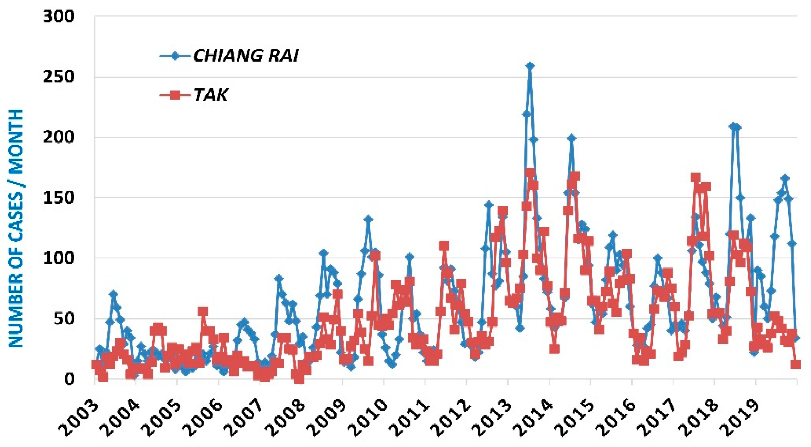
For our analysis, we retain as the date the one associated with the entry to the hospital. The number of cases considered at too high a spatial scale of resolution leads to unpredictable processes. Aggregating data at the provincial level and for each month is a good compromise between structuring a consistent signal and sufficient length of the time series. Figure 1 shows the series obtained for two provinces in northern Thailand. The patterns of these two time-series are similar to those obtained for the other provinces (as well as for the whole Thailand time series) where scrub typhus is endemic. The number of cases is low until 2006–2007. Then the annual cycle becomes wider, with a strong annual variability. A decrease in the cycle in 2016 and 2017 is not confirmed in the following years. We can also see a non-linear rise in the base level, which we will consider to be a trend. Our analysis focuses on those provinces where the number of cases (which we will sometimes call “incidence” a little improperly but for better readability of the text) is relatively high. In fact, the majority of the 76 provinces only present very sporadic and low incidence episodes. For this same reason, the prediction and the prevention that could make use of it are not suitable for prompting the implementation of dedicated public health measures.
3. Incidence Time Series Modelling
The ARIMA (autoregressive integrated moving average model), ARFIMA (autoregressive fractionally integrated moving average) and fractional Brownian motion(fBm) models are briefly described followed by the three criteria used to select the best performing candidate for making predictions. The ARIMA time series prediction method was proposed by Box and Jenkins in the 1970s [12]. In general, a stationary sequence can establish a metrology model. The unit root test is used to evaluate the stationarity of the sequence. Some non-stationary sequences are convertible in stationary sequences with one or several applications of a difference operation (subtracting the previous datum to the current one). A difference-stationary or unit root I(D) process is a process that makes a sequence stationary by taking D differences, the integer D being the degree of the model. The ARIMA (p, D, q) model is essentially a combination of difference operations and ARMA (p, q) model (linear combination of the previous p terms for the autoregressive polynomial in the lag operator, and updated q terms entering the moving average polynomial). After transforming the original data in a stationary time series (when possible), an ARIMA model is sought by estimating its parameters. The data autocorrelation and partial autocorrelation functions are used to estimate the (p,q) parameters. Then the polynomial coefficients of the model are estimated using a least squares or maximum likelihood method [13,14].
The ARFIMA model [15] is a good candidate for data time series with long-term memory. Recently, Kartikasari et al. [16] successfully applied ARFIMA models to predict the occurrence of new cases of patients dying from coronavirus disease 2019 (COVID-19) in Indonesia over a 3-month period. In contrast with ARIMA model, the differencing parameter d which governs the memory of the process is fractional (not integer; [17]) and reflects a property inherent to the processed time series. The type of time series (coloured noise) and model’s degrees of freedom required to ensure an accurate prediction of the time series must be determined (with semi-parametric estimators, [18]). Parameter d is estimated by a nonlinear least squares method using time-domain approach [19]. The (p,q) values and coefficients of the ARIMA (p,D,q) and ARFIMA (p,d,q) model are estimated with the Software EViews 3 [20].
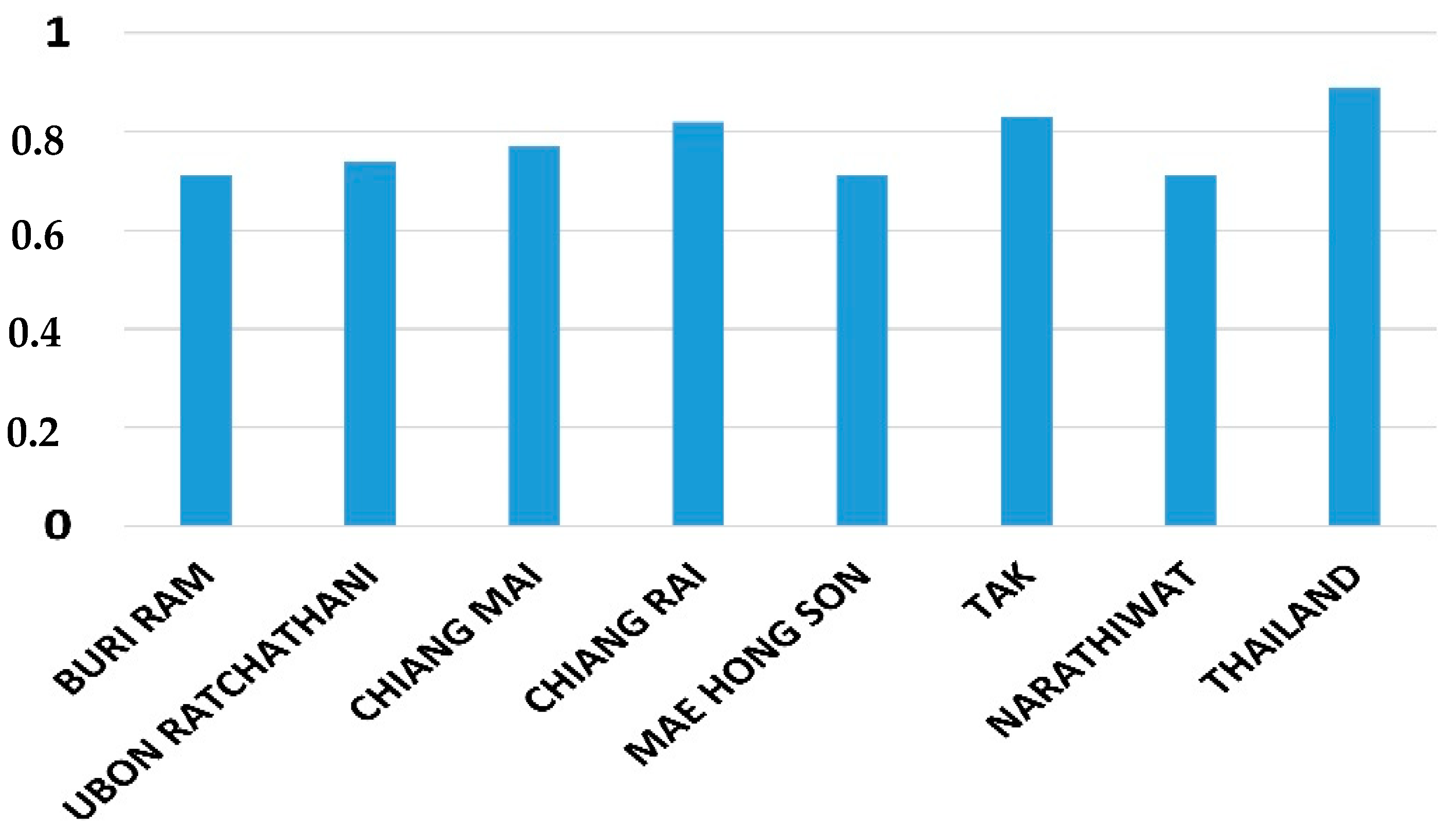
Hurst exponent H is a measure of the long-term memory of the stochastic process underlying a time series. A value of H = 0.5 indicates the lack of memory in the data (Wiener process, white noise). The closer the value of H to 1, the higher the persistence of long-term addiction (positive correlation). The data sample exhibits a persistent behavior when 0.5 < H ≤ 1. In such case, if the series increases (decreases) in the previous period, then there is a significant probability that it will maintain this tendency for some time in the immediate future. By contrast, the range 0 ≤ H < 0.5 corresponds to an anti-persistent series (negative correlation), a behaviour all the more marked as H approaches zero. There are several methods for estimating the Hurst exponent of time series with different sizes [21,22,23]. Figure 2 provides the highest Hurst exponents found at the province level in Thailand.
The forecasting of the values of a Fractional Brownian Motion is possible only for the persistent case. Indeed, the fBm [24,25] generalizes Brownian motion with time increments not necessarily independent. fBm probability distribution is self-similar. It is a function of the Hurst exponent as is fBm autocorrelation. Having a null expectation, its use as a model of empirical time series requires the prior withdrawal of the data trend. We model the data trend with an ARIMA process. The Hurst exponents and fBm models are estimated with a R-package [26,27,28].
In the test phase of candidate models, predictions of the number of scrub typhus cases are made on dates for which we already have actual observed data. Each model is optimized based on the data of the learning window and the prediction is performed for the following h_p = 1 to h_p = 14 months (h_p denoting a prediction horizon). By doing this over the entire length of a time series of observations, we can estimate the average performance of each model and compare it with that of other models. For this we use the following three criteria. Conventionally, the criterion R2 (or coefficient of determination) measures the proportion of variance of the observed data which is explained by a model (here in predictive mode). The criterion R2 takes the value 1 when the data explained (or predicted) coincide exactly with the observations. The Akaike criterion is a measure of the compromise established between the good fit of the data by a model (using a R2-like criterion) and the parametric frugality of the model. Indeed, too many parameters can lead to an adjustment which integrates noise but too few parameters do not allow us to adjust to all the variability of the signal. When comparing models fitted to the same time series, the one with the lowest Akaike criterion value is to be preferred. The Durbin–Watson test is also applied in order to check that the residues (observed minus predicted data) are not correlated (which would introduce an estimation bias of the R2 performance criterion of the model, while omitting a fraction of the signal). A value of 2 of the test indicates that the residuals are fully uncorrelated. These criteria or tests are applied to all models combined with the learning windows in order to estimate their relative predictive performances. Used in conjunction, they provide a good basis for selecting a model for predicting the number of scrub typhus cases.
4. Incidence Predictability: Results
Three models are in competition: ARIMA, ARFIMA and fBm combined with an ARIMA model to capture the trend of time series (this combined model is denoted fBm*). We rule out the fBm model alone because it does not correctly reproduce the trend of the time series. Each model is optimized to fit the number of cases monthly data in a so-called learning window. The length q of these windows, of 12 (one year), 25 or 50 months (a little more than two and four years respectively), is attached to the label assigned to each model. Adjustments on training sets of q = 6 months have not given satisfactory results and are ruled out. They do not even adequately capture the annual cycle of scrub typhus incidences.
Once adjusted to the monthly data of the training window, a model is used to predict the number of scrub typhus cases over the next 14 months. As the predictions being made in past years, they can be compared to available data of the Thai Ministry of Public Health. The procedure is repeated throughout the data time series. The performances of the different models are thus evaluated and compared. The results are presented here for a prediction horizon h_p ranging from 1 to 3 months, a period of anticipation of incidences useful for the implementation of preventive health measures. Naturally, the performance of the models deteriorates for longer-term predictions. The inspection of the results does not show any exploitable results for longer horizons (h_p ≥ 4), which the dominance of the incidences’ annual cycle and inter-annual variability could allow one to hope.
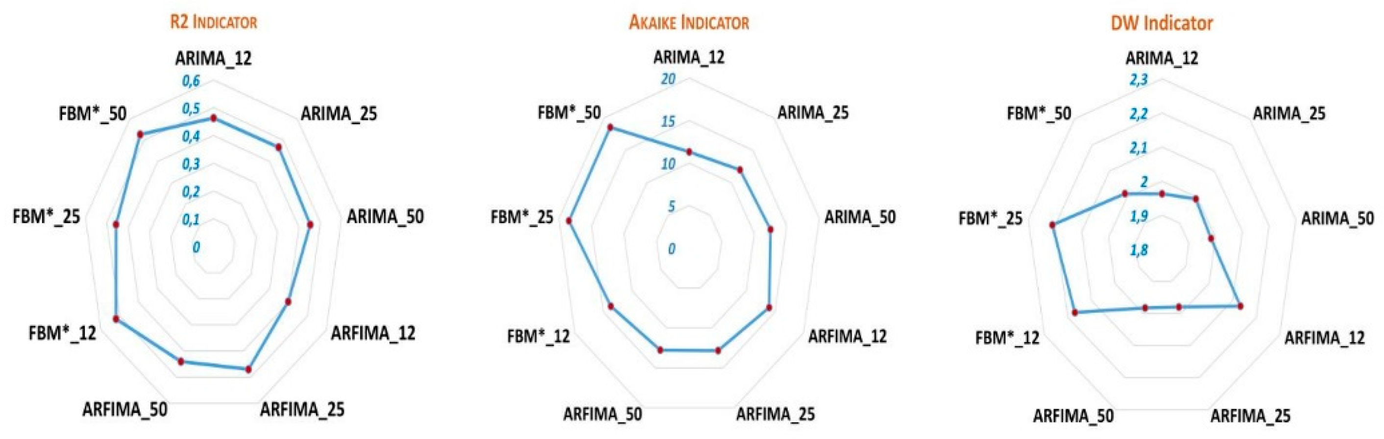
National level: each of the three models is applied with the three learning windows to the data aggregated at the Thailand level. To compare the performance of the models and their configuration of use, the values of R2 of the prediction horizons of 1, 2 and 3 months are averaged to give a “R2 indicator”. This procedure makes it possible consider the best score—obtained for h_p = 1 month—but also the decrease in this score over the period of interest for health prevention. The same procedure is used to produce an Akaike indicator and a Durbin–Watson indicator. The results are collated in Figure 3 for comparison.
In most cases, the comparison of entities on the basis of three criteria does not constitute an order relation which would unambiguously designate the entity to be retained, but a partial order [29]. Because it directly concerns the prediction of the number of people affected by scrub typhus, we will primarily consider the score of R2 indicator, and use the other two indicators in addition. The sole Akaike’s indicator would systematically disqualify the fBm* model which combines the parameters of a fBm model and of an ARIMA model for the trend. However, fBm* gives results of the same order as the other candidates in terms of R2 or Durbin–Watson indicators (whereas ARIMA or ARFIMA models associated with a similar Akaike criterion perform less in terms of R2).
Among the nine configurations tested, fBm*_50 presents the best R2 indicator (and criterion with R2 = 0.57 for h_p = 1) as well as fBm*_25 in second position. Unsurprisingly, these two models have a number of parameters which tend to disqualify them compared to other models, in particular ARFIMA_12. However, with a DW indicator of 2.01, (2.21 for fBm*_25 and 2.13 for ARFIMA_12), it turns out to be our preferred candidate. On the other hand, the configuration using training windows of q = 12 months leads to models that leave correlated prediction residuals (DW indicator furthest from 2). It is excluded from analyses at the province level.
Provincial level: we focus here on four provinces with high Hurst exponents (Table 1). These are also provinces where the number of people infected is the highest each year, while some other provinces have almost no cases. Provincial government bodies enjoy the autonomy necessary to implement preventive health measures in their territory. Therefore, it is at this administrative scale that prediction may be the most useful and effective. By comparing the performance of the models for each province as we did previously (with q = 25 and q = 50 learning windows), we end up with the selection of models presented in Table 1. Except for the province of Tak, the R2 indicators are higher than 0.5. The best score (0.62) is obtained in Chiang Mai, a province of northern Thailand. The R2 associated with the only prediction horizon h_p = 1 month is 0.72.
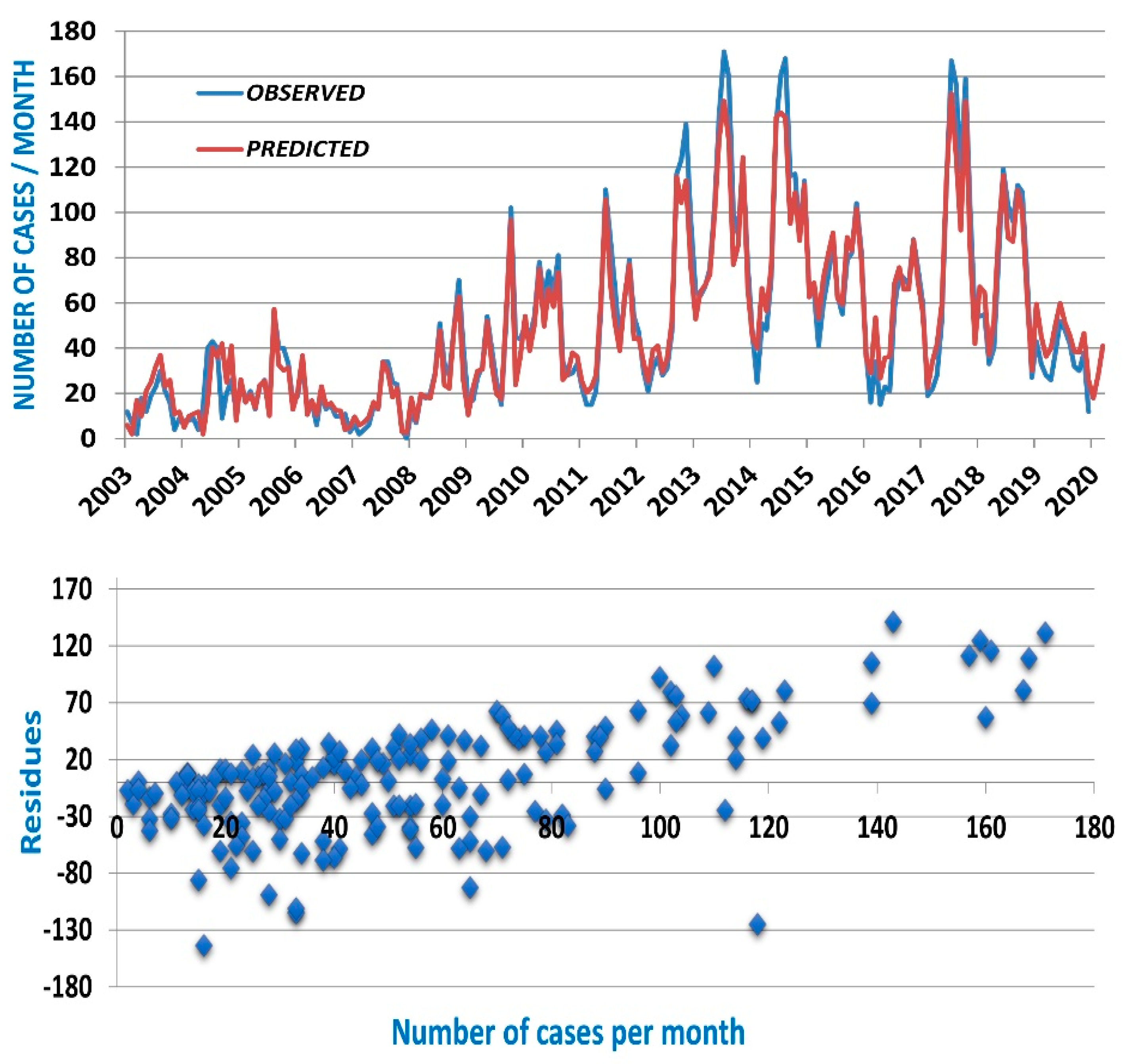
The other provinces show scores comparable to those of Thailand, although their Hurst exponent, and therefore the memory measure of the number of people infected with scrub typhus, is significantly lower. The Durbin–Watson indicator indicates a lack of correlation of the residuals, and the Akaike indicator primarily reports the number of parameters in each model. Figure 4 shows as an example the observed time series of Tak province, the predicted data with 3 months of antecedence (h_p = 3) as well as the scatter plot of the prediction residues.
Very similar figures are obtained for the other provinces and for Thailand. The number of scrub typhus cases is a positive variable. The models predict fairly well the local minima of the series, associated with the months of December through April of the following year. The scatter diagram (Figure 4 bottom) shows that the maxima are almost systematically underestimated. The models provide a low estimate of the number of scrub typhus cases to come in the following months which, in itself, is useful information for provincial governments. However, this is another observation that catches our attention. It is neither always the same type of model (fBm* or ARFIMA), nor the same training length (q = 25 or q = 50), which offers the best predictive capacity. Added to this is the fact that in some provinces an ARIMA model has a performance only slightly inferior to that of the best model. On the other hand, nothing in Table 1 indicates that a long learning window is preferable when the Hurst exponent is higher, neither that national-level data aggregation is more predictable (compare models’ performances in Chiang Mai or Chiang Rai with Thailand). Nevertheless, the results show that models are available to produce a low estimate of the number of scrub typhus cases in the next 2 or 3 months in the provinces where the disease is endemic and has the highest incidence.
Thailand Overview and Discussion
None of our results militate in favour of a “universal” model, in the sense that it would apply to all provinces with equal success and would emerge as the best representation of the epidemic dynamics of scrub typhus, at least in Thailand. It should also be remembered that in most provinces the series are generally not stationary, nor can they even be transformed into stationary series. Our understanding, therefore, tends more in the direction of an out-of-equilibrium dynamic, somewhat latent (weak background signal), which would take off towards a more stable regime in favour of contingent local ecological, social and environmental conditions. It is the establishment of this stable regime and time series regular behaviour that would condition the capacity to predict with a few months of antecedence the number of scrub typhus cases, aggregated at the correct spatial and temporal scales (in this case the province and the month).
Therefore, the most useful strategy is to select a model and a learning window adjusted to each province whose Hurst exponent is greater than a threshold value (e.g., H_threshold = 0.6). The prediction horizon must also be adapted to each provincial context so as to operationalize a compromise between: (1) an acceptable level of performance for the predictions; (2) taking into account the incubation times of the disease and diagnosis in a hospital; (3) taking into account the delays for implementing public health measures aimed at preventing the resurgence of cases and reducing the incidence of scrub typhus.
The preventive public health actions, scaled according to the low estimates of the predictions, could be implemented by the authorities in the districts where the cases are concentrated rather than at the level of an entire province. Data analysis identifies those districts whose relatively persistent ecological and social factors favour the annual recurrence of local scrub typhus epidemics. Let us add that the results presented here give a reference level against which to develop other more efficient modelling approaches (if there are any). Along with other model performance indicators that may obscure their ultimate utility, the production of reliable predictions of scrub typhus incidences remains both an excellent criterion for qualifying models and a challenge for research.
5. Conclusions
In the Thai provinces where scrub typhus is endemic, the prediction of the monthly number of cases is a public health issue of interest for implementing preventive measures. Applying a difference operation makes the observed data time series stationary. The selected series have a Hurst exponent greater than 0.7 and, therefore, a long-term memory making them suitable for a prediction over horizons of several months. The ARIMA, ARFIMA and fBm models of these time series, adjusted on moving training windows of approximately 1, 2 and 4 years, are put in competition in order to identify the best prediction options and evaluate their performance from three criteria (R2, Akaike and Durbin–Watson). Predictions for horizons spanning 1 to 14 months are compared to existing observations (up to 2019). The results obtained allow operational use of the predictions of scrub typhus epidemic events in the provinces concerned with up to three months of antecedent. However, it is neither the same model nor the same size of learning window that give the best predictions from province to province. The performance of the models presented constitutes a benchmark against which several improvement strategies are possible. These analyses also suggest that the ability to predict the number of scrub typhus cases (and even of other infectious diseases) several months in advance is a real challenge that modelling should not avoid.
Author Contributions
Conceptualization, V.B. and P.M.; methodology, V.B. and P.M.; software, validation and formal analysis, V.B.; writing—review and editing, P.M., C.L.; supervision, P.M., C.L. All authors have read and agreed to the published version of the manuscript.
Funding
This research was funded by the Agence Nationale de la Recherche, Research project FutureHealthSEA “Predictive scenarios of health in Southeast Asia: linking land use and climate changes to infectious diseases”, ANR-17-CE35-0003-01.
Acknowledgments
We gratefully thank H. Soawapak for giving us the opportunity to access the data and R. Kumlert, for providing the selected data, both at the Department of Disease Control, Ministry of Public Health in Thailand.
Conflicts of Interest
The authors declare no conflict of interest.
References
- Acestor, N.; Cooksey, R.; Newton, P.N.; Menard, D.; Guerin, P.J.; Nakagawa, J.; Christophel, E.; Gonzalez, I.J.; Bell, D. Mapping the aetiology of non-malarial febrile illness in Southeast Asia through a systematic review—Terra Incognita impairing treatment policies. PLoS ONE 2012, 7, e44269. [Google Scholar] [CrossRef] [Green Version]
- Aung, A.K.; Spelman, D.W.; Murray, R.J.; Graves, S. Rickettsial infections in Southeast Asia: Implications for local populace and febrile returned travelers. Am. J. Trop. Med. Hyg. 2014, 91, 451–460. [Google Scholar] [CrossRef] [PubMed]
- Prompiram, P.; Poltep, K.; Pamonsupornvichit, S.; Wongwadhunyoo, W.; Chamsai, T.; Rodkvamtook, W. Rickettsiae exposure related to habitats of the oriental house rat (Rattus tanezumi, Temminck, 1844) in Salaya suburb, Thailand. Int. J. Parasitol. Parasites Wildl. 2020, 13, 22–26. [Google Scholar] [CrossRef] [PubMed]
- Xu, G.; Walker, D.H.; Jupiter, D.; Melby, P.C.; Arcari, C.M. A review of the global epidemiology of scrub typhus. PLoS Negl. Trop. Dis. 2017, 11, e0006062. [Google Scholar] [CrossRef] [PubMed] [Green Version]
- Bonell, A.; Lubell, Y.; Newton, P.N.; Crump, J.A.; Paris, D.H. Estimating the burden of scrub typhus: A systematic review. PLoS Negl. Trop. Dis. 2017, 11, e0005838. [Google Scholar] [CrossRef] [PubMed] [Green Version]
- Wangrangsimakul, T.; Elliott, I.; Nedsuwan, S.; Kumlert, R.; Hinjoy, S.; Chaisiri, K.; Day, N.; Morand, S. The estimated burden of scrub typhus in Thailand from national surveillance data (2003–2018). PLoS Negl. Trop. Dis. 2020, 14, e0008233. [Google Scholar] [CrossRef] [PubMed] [Green Version]
- Gao, J.; Li, J.; Wang, M. Time series analysis of cumulative incidences of typhoid and paratyphoid fevers in China using both Grey and SARIMA models. PLoS ONE 2020, 15, e0241217. [Google Scholar] [CrossRef] [PubMed]
- Allard, R. Use of time-series analysis in infectious disease surveillance. Bull World Health Organ. 1998, 76, 327–333. [Google Scholar] [PubMed]
- Holloway, R.; Rasmussen, S.A.; Zaza, S.; Cox, N.J.; Jernigan, D.B. Updated preparedness and response framework for influenza pandemics. MMWR. Recommendations and reports. MMWR Morb. Mortal. Wkly. Rep. Recomm. Rep. 2014, 63, 1–18. [Google Scholar]
- Lutz, C.S.; Huynh, M.P.; Schroeder, M.; Anyatonwu, S.; Dahlgren, F.S.; Danyluk, G.; Fernandez, D.; Greene, S.K.; Kipshidze, N.; Liu, L.; et al. Applying infectious disease forecasting to public health: A path forward using influenza forecasting examples. BMC Public Health 2019, 19, 1659. [Google Scholar] [CrossRef] [PubMed] [Green Version]
- Fischer, L.S.; Santibanez, S.; Hatchett, R.J.; Jernigan, D.B.; Meyers, L.A.; Thorpe, P.G.; Meltzer, M.I. CDC Grand Rounds: Modeling and public health decision-making. MMWR Morb. Mortal. Wkly. Report. 2016, 65, 1374–1377. [Google Scholar] [CrossRef] [PubMed] [Green Version]
- Box, G.E.P.; Jenkins, G.M. Time Series Analysis Forecasting and Control; Holden-Day: San Francisco, CA, USA, 1970. [Google Scholar]
- Beran, J. Statistics for Long-Memory Processes; Chapman and Hall: London, UK, 1994. [Google Scholar]
- Hyndman, R.; Koehler, A.B.; Ord, J.K.; Snyder, R.D. Forecasting with Exponential Smoothing: The State Space Approach; Springer: Berlin, Germany, 2008. [Google Scholar]
- Granger, C.W.J.; Joyeux, R. An Introduction to Long-Range Time Series Models and Fractional Differencing. J. Time Ser. Anal. 1980, 1, 15–29. [Google Scholar] [CrossRef]
- Kartikasari, P.; Yasin, H.; Maruddani, D.A. ARFIMA model for short term forecasting of new death cases COVID-19. In E3S Web of Conferences; EDP Sciences: Paris, France; London, UK, 2020; Volume 202, p. 13007. [Google Scholar]
- Hosking, J.R.M. Fractional differencing. Biometrika 1981, 68, 165–176. [Google Scholar] [CrossRef]
- Robinson, P.M. (Ed.) Time Series Analysis with Long Memory; Oxford University Press: Oxford, UK, 2003. [Google Scholar]
- Breidt, F.J.; Crato, N.; De Lima, P. The detection and estimation of long memory in stochastic volatility. J. Econom. 1998, 83, 325–348. [Google Scholar] [CrossRef] [Green Version]
- Ma, L.; Hu, C.; Lin, R.; Han, Y. ARIMA model forecast based on EViews software. IOP Conf. Ser. Earth Environ. Sci. 2018, 208, 012017. [Google Scholar] [CrossRef]
- Willinger, W.; Taqqu, M.; Erramilli, A. Bibliographical guide to self-similar traffic and performance modeling for modern high-speed network. In Stochastic Networks: Theory and Applications; Kelly, F.P., Zachary, S., Ziedins, I., Eds.; Claredon Press—Oxford University Press: Oxford, UK, 1996; Chapter 20; pp. 339–366. [Google Scholar]
- Clegg, R.G. A practical guide to measuring the Hurst parameter. Int. J. Simul. Syst. Sci. Technol. 2005, 7, 3–14. [Google Scholar]
- Coeurjolly, J.-F. Hurst exponent estimation of locally self-similar Gaussian processes using sample quantiles. Ann. Stat. 2008, 36, 1404–1434. [Google Scholar] [CrossRef]
- Mandelbrot, B.; van Ness, J.W. Fractional Brownian motions, fractional noises and applications. SIAM Rev. 1968, 10, 422–437. [Google Scholar] [CrossRef]
- Mishura, Y. Stochastic Calculus for Fractional Brownian Motion and Related Processes; Lecture Notes in Mathematics; Springer: Berlin, Germany, 2008. [Google Scholar]
- Buhovets, A.G.; Moskalev, P.V.; Bogatova, V.P.; Ya Biryuchinskaya, T. Statistical Analysis of the Data in the R; VGAU: Voronezh, Russia, 2010. [Google Scholar]
- McLeod, A.I.; Yu, H.; Mahdi, E. Time Series Analysis with R. Time Ser. Anal. Methods Appl. 2012, 30, 661–712. [Google Scholar] [CrossRef]
- Shang, H.L. FTSA: An R package for analyzing functional time series. R J. 2013, 5, 64–72. [Google Scholar] [CrossRef] [Green Version]
- Mazzega, P.; Lajaunie, C.; Leblet, J.; Barros-Platiau, A.F.; Chansardon, C. How to compare bundles of national environmental and development indexes? In Law, Public Policies and Complex Systems: Networks in Action; Boulet, R., Lajaunie, C., Mazzega, P., Eds.; Law, Gov. & Tech. Series 16; Springer: Berlin, Germany, 2019; pp. 243–265. [Google Scholar]
Figure 1.
Time series of the number of cases of scrub typhus per month from January 2003 to December 2019 in Chiang Rai and Tak provinces.
Figure 1.
Time series of the number of cases of scrub typhus per month from January 2003 to December 2019 in Chiang Rai and Tak provinces.

Figure 2.
Hurst exponents for Thailand and provinces with H > 0.7 and stationary scrub typhus incidence time series.
Figure 2.
Hurst exponents for Thailand and provinces with H > 0.7 and stationary scrub typhus incidence time series.

Figure 3.
R2, Akaike and Durbin–Watson (DW) indicators of ARIMA (autoregressive integrated moving average model, ARFIMA (autoregressive fractionally integrated moving average) and fbm plus ARIMA-trend” (labelled fBm*) models’ performances for 3 learning windows (12, 25 and 50 months) with Thailand level incidence data (see text).

Figure 4.
(Top) Observed and predicted time series of scrub typhus cases for Tak province with ARFIMA_25 model and hp = 3 months; (Bottom) scatter plot of the residues (observed minus predicted data).
Figure 4.
(Top) Observed and predicted time series of scrub typhus cases for Tak province with ARFIMA_25 model and hp = 3 months; (Bottom) scatter plot of the residues (observed minus predicted data).


Table 1.
Best models for provinces with Hurst exponents higher than 0.7, and their performance indicators. The R2 score for h_p = 1 is given in parenthesis.
Table 1.
Best models for provinces with Hurst exponents higher than 0.7, and their performance indicators. The R2 score for h_p = 1 is given in parenthesis.
| Province | Hurst | Best Model | R2|Akaike|DW Indicators | |
|---|---|---|---|---|
| U. Ratchathani | 0.74 | fBm_25 | 0.52 (0.53)|16.05|2.02 | |
| Chiang Mai | 0.77 | ARFIMA_50 | 0.62 (0.72)|9.70|1.99 | |
| Chiang Rai | 0.82 | fBm*_50 | 0.59 (0.63)|20.10|2.02 | |
| Tak | 0.83 | ARFIMA_25 | 0.47 (0.51)|10.22|1.97 | |
| Thailand | 0.93 | fBm*_50 | 0.53 (0.57)|18.55|2.01 |
Publisher’s Note: MDPI stays neutral with regard to jurisdictional claims in published maps and institutional affiliations. |
© 2021 by the authors. Licensee MDPI, Basel, Switzerland. This article is an open access article distributed under the terms and conditions of the Creative Commons Attribution (CC BY) license (https://creativecommons.org/licenses/by/4.0/).
Share and Cite
MDPI and ACS Style
Bondarenko, V.; Mazzega, P.; Lajaunie, C. Predictability of Scrub Typhus Incidences Time Series in Thailand. Eng. Proc. 2021, 5, 44. https://0-doi-org.brum.beds.ac.uk/10.3390/engproc2021005044
AMA Style
Bondarenko V, Mazzega P, Lajaunie C. Predictability of Scrub Typhus Incidences Time Series in Thailand. Engineering Proceedings. 2021; 5(1):44. https://0-doi-org.brum.beds.ac.uk/10.3390/engproc2021005044
Chicago/Turabian StyleBondarenko, Valeria, Pierre Mazzega, and Claire Lajaunie. 2021. "Predictability of Scrub Typhus Incidences Time Series in Thailand" Engineering Proceedings 5, no. 1: 44. https://0-doi-org.brum.beds.ac.uk/10.3390/engproc2021005044