Water Quality Monitoring with Arduino Based Sensors

 , , , , and
Abstract
:1. Introduction
- Sediment washing from agriculture.
- Deadly viruses and bacteria from animal grazing.
- Construction works.
- Aftermath of natural disasters particularly floods, tornadoes, hurricanes, and tsunamis.
- Gasoline and oil from recreational boating.
- Old and leaky septic systems.
- Urban runoffs from homes and landfills.
- Chemicals from household mismanagement and so on.
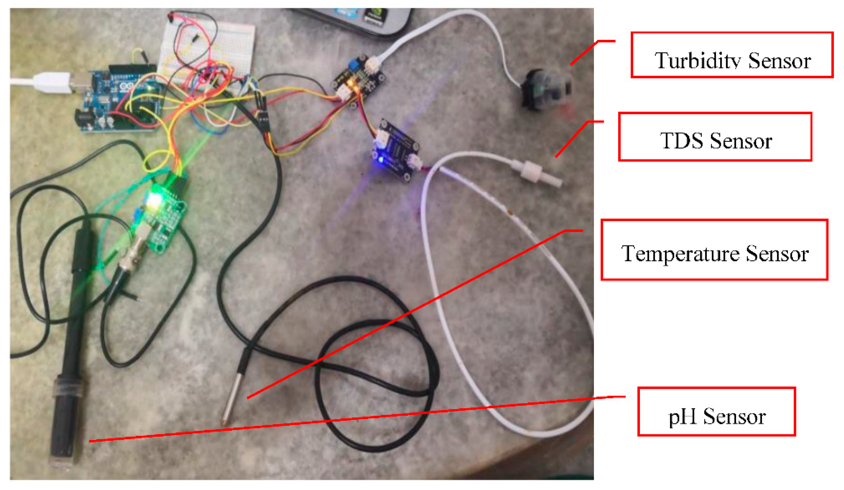
2. Design and Development
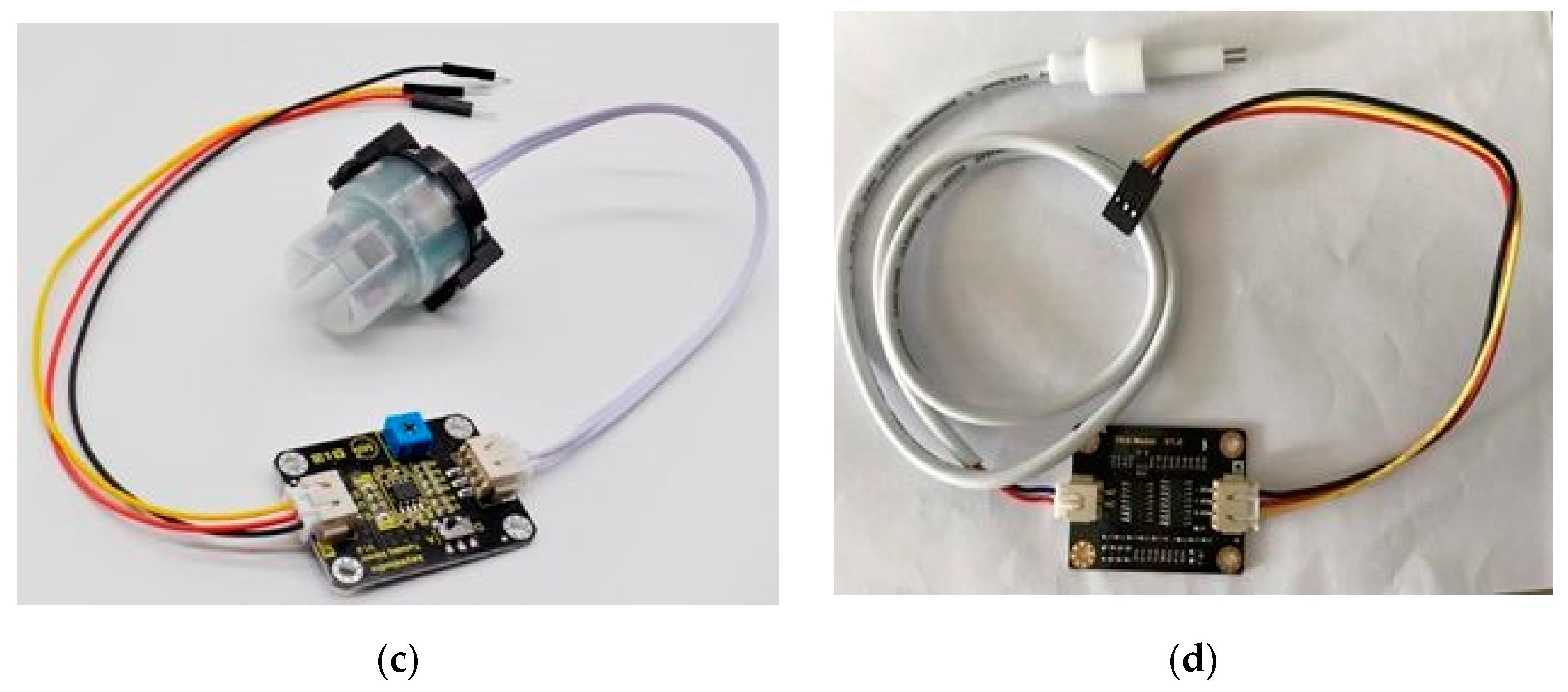
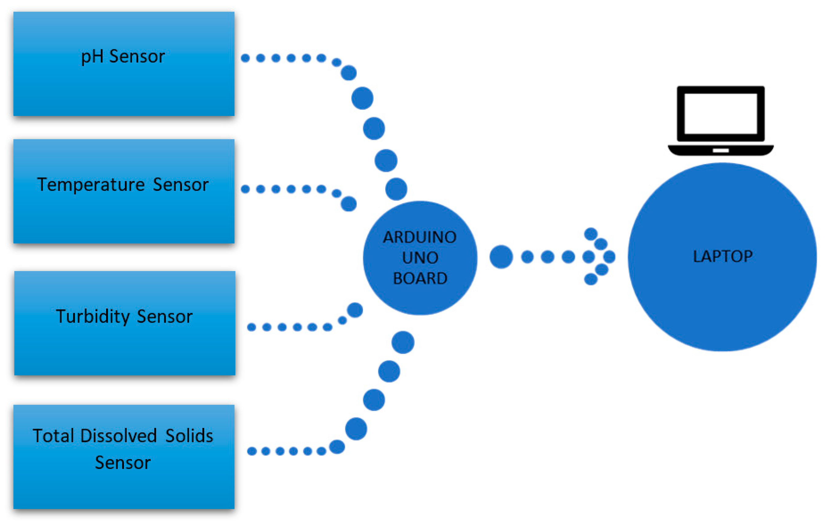
- Multiple sensors to collect relevant data from the environment.
- A central microcontroller loaded with a computer program to read analogue data and convert them to digital output.
- A portable laptop with relevant software to read the digital data and present the data in an understandable format on a screen, as well as to provide power to the microcontroller.
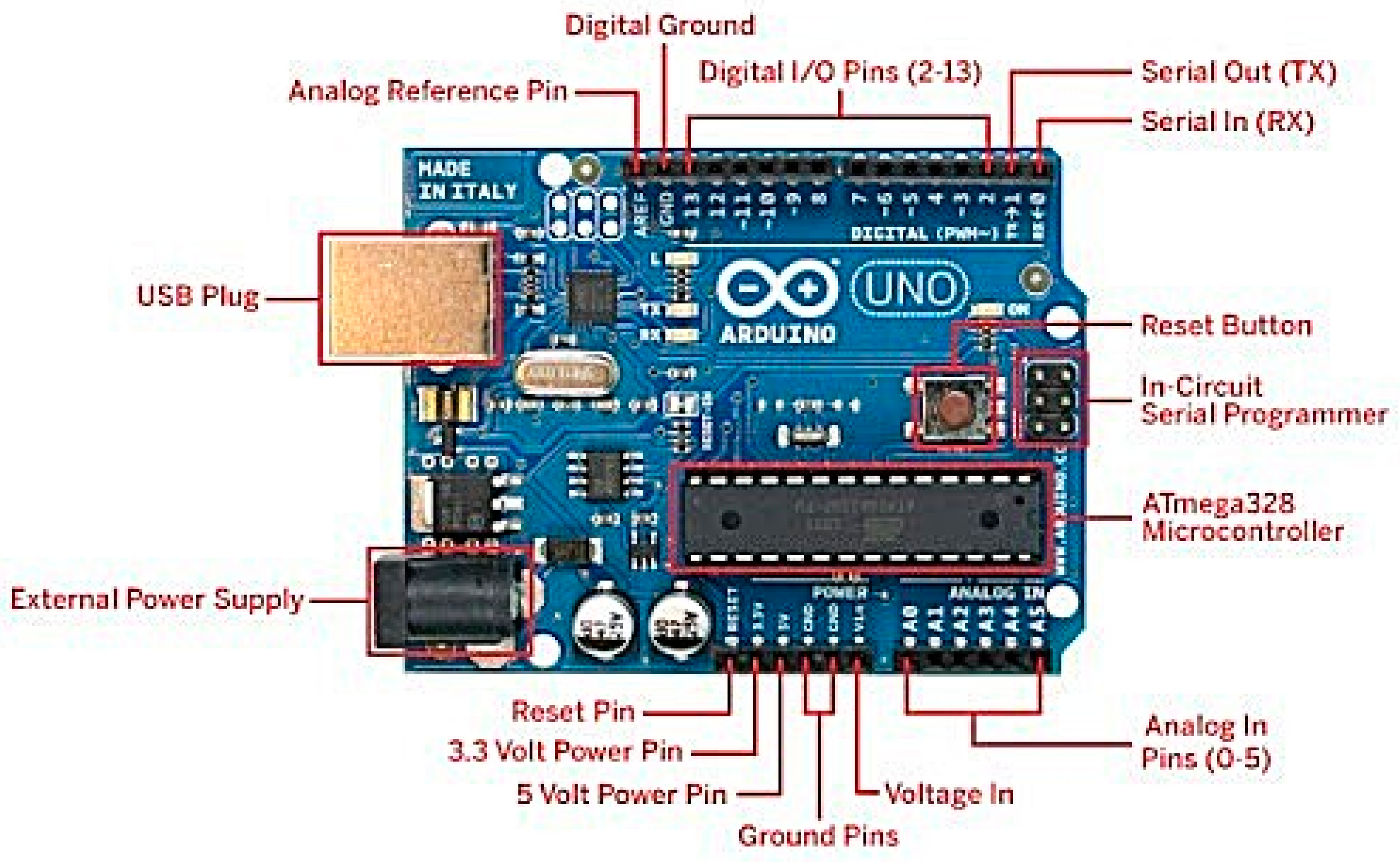
- A total of 6 analog input pins labelled A0 to A5 to allow up to a maximum of 6 analog sensors to connect directly to the Arduino.
- A total of 2 power supplies pin labelled 3.3 volts and 5 volts with in-built voltage regulation to provide power to sensors.
- A USB plug that can be used in conjunction with a USB cable to connect with a microprocessor.
3. Results
4. Discussion
5. Conclusions
Author Contributions
Funding
Conflicts of Interest
References
- McClelland, C. What Is IoT? A Simple Explanation of the Internet of Things. Available online: https://www.iotforall.com/what-is-iot-simple-explanation/ (accessed on 13 May 2019).
- Diène, B.; Rodrigues, J.J.P.C.; Diallo, O.; Ndoye, E.H.M.; Korotaev, V.V. Data management techniques for Internet of Things. Mech. Syst. Signal Process. 2020, 138, 106564. [Google Scholar] [CrossRef]
- McClelland, C. IoT Explained—How Does an IoT System Actually Work? Available online: https://www.leverege.com/blogpost/iot-explained-how-does-an-iot-system-actually-work (accessed on 29 October 2016).
- Li, C.-Z.-E.; Deng, Z.W. The Embedded Modules Solution of Household Internet of Things System and The Future Development. Procedia Comput. Sci. 2020, 166, 350–356. [Google Scholar] [CrossRef]
- Dachyar, M.; Zagloel, T.; Saragih, L. Knowledge Growth and Development: Internet of Things (Iot) Research, 2006–2018. Heliyon 2020, 5, e02264. [Google Scholar] [CrossRef] [PubMed] [Green Version]
- Cipolla, S.; Maglionico, M.; Masina, M.; Lamberti, A.; Daprà, I. Real time monitoring of water quality in an agricultural area with salinity problems. Environ. Eng. Manag. J. 2019, 18, 2229–2240. [Google Scholar]
- Pal, A.; Kant, K. Water flow Driven Sensor Networks for leakage and contamination monitoring. In Proceedings of the 2015 IEEE 16th International Symposium on A World of Wireless, Mobile and Multimedia Networks (WoWMoM), Boston, MA, USA, 14–17 June 2015. [Google Scholar] [CrossRef]
- IoT Smart City—What Is Smart Home? The Internet of Things. Available online: http://www.infiniteinformationtechnology.com/iot-smart-city-what-is-smart-home (accessed on 27 November 2016).
- Mallon, S. IoT Is the Most Important Development of the 21st Century. Available online: https://www.smartdatacollective.com/iot-most-important-development-of-21st-century/ (accessed on 29 October 2018).
- Ranger, S. What Is the IoT? Everything You Need to Know about the Internet of Things Right Now. Available online: https://www.zdnet.com/article/what-is-the-internet-of-things-everything-you-need-to-know-about-the-iot-right-now/ (accessed on 21 August 2018).
- Everard, M.; Powell, A. Rivers as living systems. Aquat. Conserv. Mar. Freshw. Ecosyst. 2002, 12, 329–337. [Google Scholar] [CrossRef]
- U.S. Environmental Protection Agency [EPA]. National Nonpoint Source Program—A Catalyst for Water Quality Improvements. Available online: https://www.epa.gov/sites/production/files/2016-10/documents/nps_program_highlights_report-508.pdf (accessed on 2 November 2020).
- Donlon, A.; McMillan, B. Best Management Practices to Control Nonpoint Source Pollution: A Guide for Citizens and Town Officials; The Watershed Assistance Section, NH Department of Environmental Services: Concord, NC, USA, 2004.
- Hader, D.P.; Barnes, P.W. Comparing the impacts of climate change on the responses and linkages between terrestrial and aquatic ecosystems. Sci. Total Environ. 2019, 682, 239–246. [Google Scholar] [CrossRef] [PubMed]
- Tornevi, A.; Bergstedt, O.; Forsberg, B. Precipitation Effects on Microbial Pollution in a River: Lag Structures and Effect Modification. PLoS ONE 2014, 9, e98546. [Google Scholar] [CrossRef] [PubMed]
- Ismail, W.; Hashim, M. Changing trends of rainfall and sediment fluxes in the Kinta River catchment, Malaysia. In Proceedings of the International Association of Hydrological Sciences, New Orleans, LA, USA, 11–14 December 2014. [Google Scholar] [CrossRef] [Green Version]
- Karr, J.R.; Fausch, K.D.; Angermeier, P.L.; Yant, P.R.; Schlosser, I.J. Assessing Biological Integrity in Running Waters: A Method and its Rationale; Special Publication 5; Illinois Natural History Survey: Champaign, IL, USA, 1986. [Google Scholar]
- Norris, R.H.; Thoms, M.C. What is river health? Freshw. Biol. 1999, 41, 197–209. [Google Scholar] [CrossRef] [Green Version]
- Azhar, A.S.; Latiff, A.H.A.; Lim, L.H.; Gödeke, S.H. Groundwater investigation of a coastal aquifer in Brunei Darussalam using seismic refraction. Environ. Earth Sci. 2019, 78, 1–17. [Google Scholar] [CrossRef]
- Gödeke, S.H.; Malik, O.A.; Lai, D.T.C.; Bretzler, A.; Mansor, N.H. Water quality investigation in Brunei Darussalam: Investigation of the influence of climate change. Environ. Earth Sci. 2020, 79, 419. [Google Scholar] [CrossRef]
- Marshall, D.J.; Abdelhady, A.A.; Wah, D.T.T.; Mustapha, N.; Gödeke, S.H.; De Silva, L.C.; Hall-Spencer, J.M. Biomonitoring acidification using marine gastropods. Sci. Total Environ. 2019, 692, 833–843. [Google Scholar] [CrossRef] [PubMed]
- Gödeke, S.; Geistlinger, H.; Fischer, A.; Richnow, H.H.; Wachter, T.; Schirmer, M. Simulation of a reactive tracer experiment using sto-chastic hydraulic conductivity fields. Environ. Geol. 2008, 55, 1255–1261. [Google Scholar] [CrossRef]
- Khalid, M. Plans to Prevent the Degradation of Water Quality in Brunei. Available online: https://borgenproject.org/water-quality-brunei/ (accessed on 31 July 2018).
- Yusri, N.I.A.B.; Gödeke, S.H.; Mohd Mansor, N.H.B.H. A water quality database for Brunei—The case of Bukit Barun and Layong. In Proceedings of the 7th Brunei International Conference on Engineering and Technology 2018 (BICET 2018), Bandar Seri Begawan, Brunei, 12–14 November 2018. [Google Scholar] [CrossRef] [Green Version]
- Spano, D.; Duce, P.; Snyder, R.L.; Cesaraccio, C. An improved model for determining degree-day values from daily temperature data. Int. J. Biometeorol. 2001, 45, 161–169. [Google Scholar] [CrossRef] [PubMed]
- Perlman, H. Turbidity in the USGS Water Science School. Available online: http://water.usgs.gov/edu/turbidity.html (accessed on 2 November 2020).
- Moore, R.D.; Spittlehouse, D.L.; Story, A. Riparian microclimate and stream temperature response to forest harvesting: A review. J. Am. Water Resour. Assoc. 2005, 41, 813–834. [Google Scholar] [CrossRef]
- Ling, T.-Y.; Soo, C.-L.; Sivalingam, J.-R.; Nyanti, L.; Sim, S.-F.; Grinang, J. Assessment of the Water and Sediment Quality of Tropical Forest Streams in Upper Reaches of the Baleh River, Sarawak, Malaysia, Subjected to Logging Activities. J. Chem. 2016, 1–13. [Google Scholar] [CrossRef]
- Poisson, A. Conductivity/salinity/temperature relationship of diluted and concentrated standard seawater. IEEE J. Ocean. Eng. 1980, 5. [Google Scholar] [CrossRef]
- Moran, S. Clean water characterization and treatment objectives. In An Applied Guide to Water and Effluent Treatment Plant Design; Elsevier: Amsterdam, The Netherlands, 2018; pp. 61–67. [Google Scholar] [CrossRef]
- Gharbi, O.; Goedeke, S.; Al-Sammaraie, M.; Al-Shahwani, S.; Cheneviere, P.; Al-Mohannadi, N.; Julien, P. Core-flood analysis of acid stimulation in carbonates: Towards effective diversion and water mitigation. In Proceedings of the International Petroleum Technology Conference, IPTC 2014: Unlocking Energy Through Innova-tion, Technology and Capability, Doha, Qatar, 19–22 January 2014; Volume 4, pp. 3270–3274. [Google Scholar] [CrossRef]
- Sazali, Y.A.; Sazali, W.M.L.; Ibrahim, J.M.; Dindi, M.; Graham, G.; Gödeke, S. Investigation of high temperature, high pressure, scaling and dissolution effects for Carbon Capture and Storage at a high CO2 content carbonate gas field offshore Malaysia. J. Pet. Sci. Eng. 2019, 174, 599–606. [Google Scholar] [CrossRef]
- Fu, X.; Finley, A.; Carpenter, S. Formation Damage Problems Associated with CO2 Flooding. In Formation Damage during Improved Oil Recovery; Gulf Professional Publishing: Oxford, UK, 2018; pp. 305–359. [Google Scholar] [CrossRef]
- Tziortzioti, C.; Amaxilatis, D.; Mavrommati, I.; Chatzigiannakis, I. IoT sensors in sea water environment: Ahoy! Experiences from a short summer trial. Electron. Notes Theor. Comput. Sci. 2019, 343, 117–130. [Google Scholar] [CrossRef]


| Category | 2016 | 2017 | 2018 | 2019 |
|---|---|---|---|---|
| Consumer | 3963.0 | 5244.3 | 7036.3 | 12863.0 |
| Business: Cross-Industry | 1102.1 | 1501.0 | 2132.6 | 4381.4 |
| Business: Vertical-Specific | 1316.6 | 1635.4 | 2027.7 | 3171.0 |
| Grand Total | 6381.8 | 8380.6 | 11196.6 | 20415.4 |
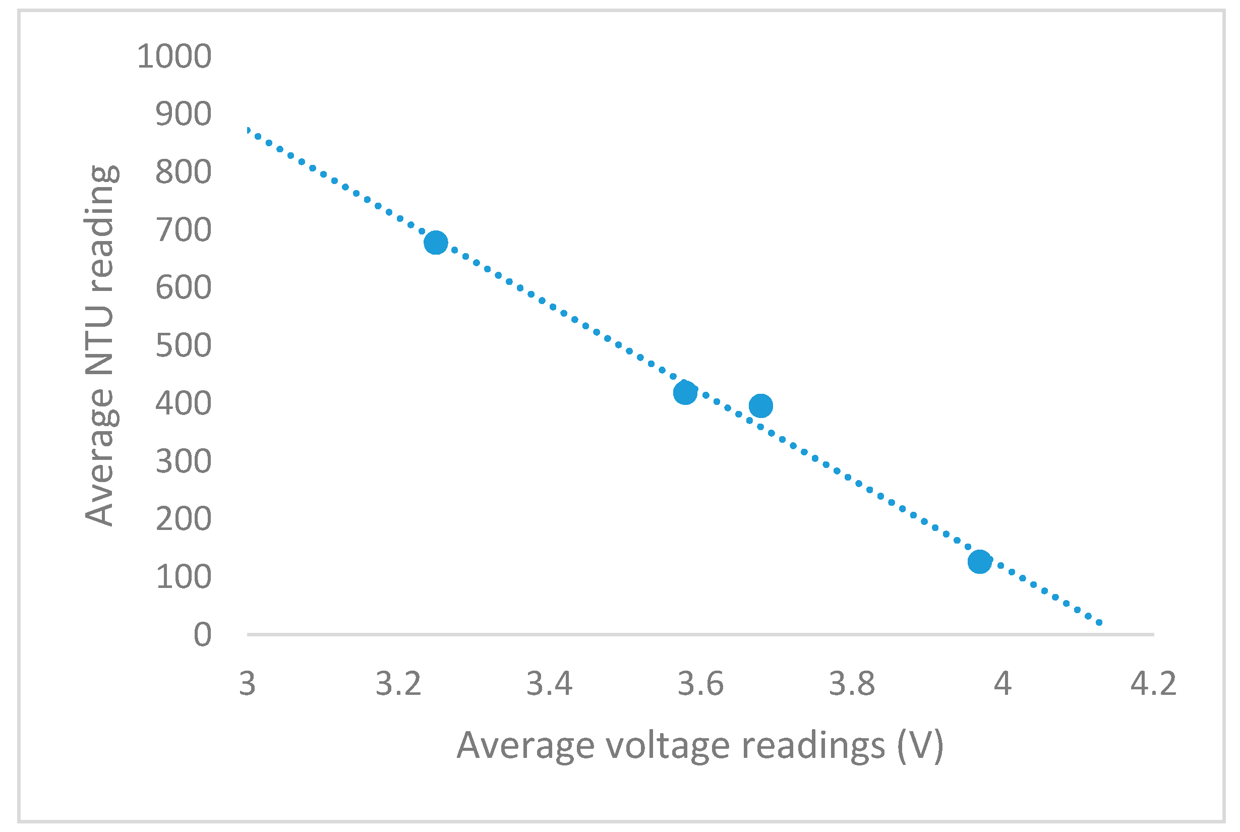
| Soil Mass (g) | Water Volume (L) | Nephelometric Turbidity Units (NTU) Readings | Average NTU Reading | Average Voltage Reading (V) |
|---|---|---|---|---|
| 1.0169 | 0.6 | 120.1, 128.3, 140.4, 121.3, 120.6 | 126.14 | 3.97 |
| 2.0190 | 0.6 | 392.0, 398.0, 392.0, 396.0, 400.0 | 395.60 | 3.68 |
| 3.0096 | 0.6 | 407.0, 422.0, 412.0, 428.0, 422.0 | 418.20 | 3.58 |
| 4.0201 | 0.6 | 677.0, 657.0, 690.0, 702.0, 664.0 | 678.00 | 3.25 |
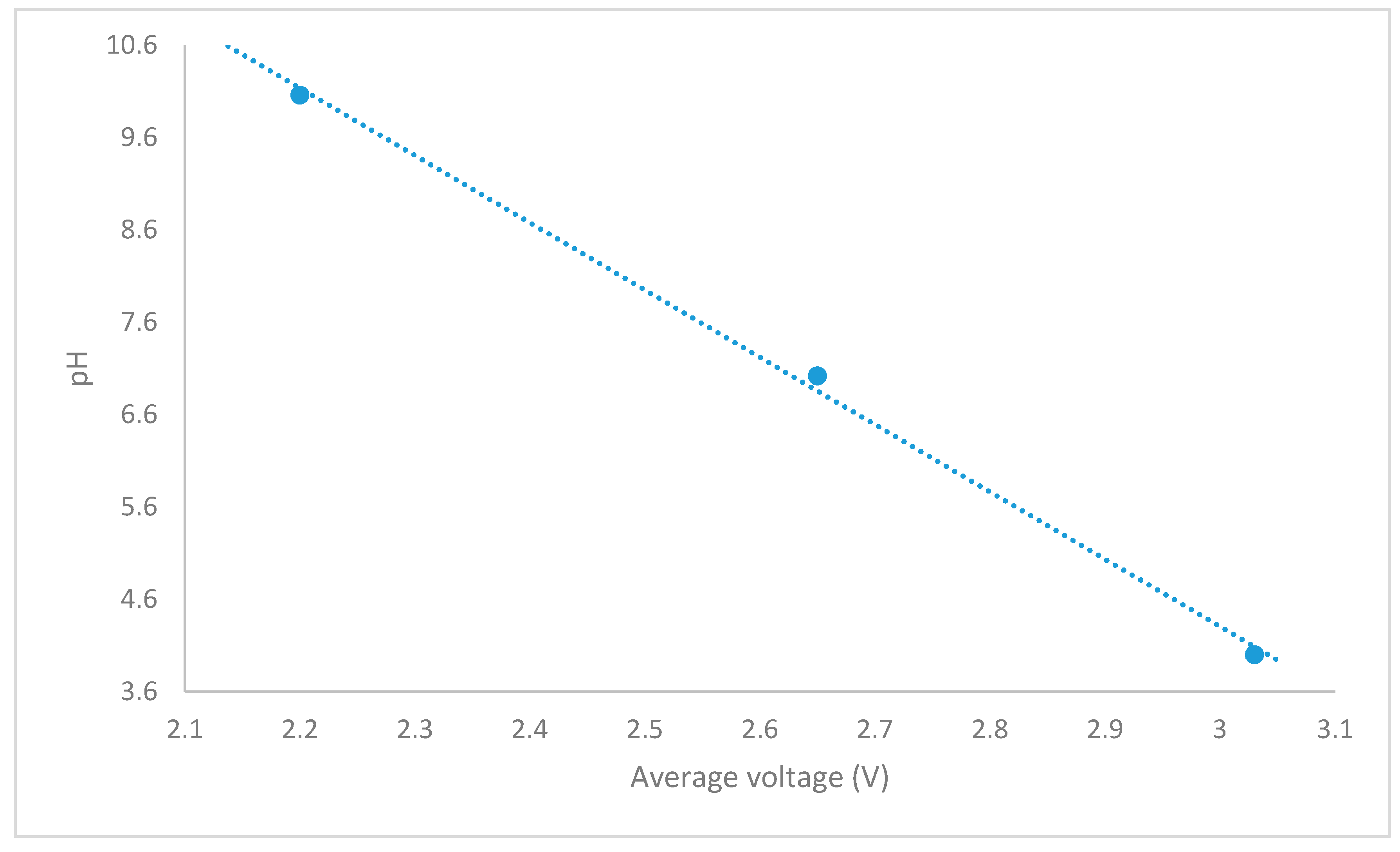
| pH | Voltage [V] | Average Voltage [V] |
|---|---|---|
| pH 10.06 | 2.20, 2.20, 2.20, 2.19, 2.20, 2.19, 2.21, 2.20, 2.20, 2.20, 2.20 | 2.20 |
| pH 7.02 | 2.69, 2.65, 2.65, 2.64, 2.65, 2.64, 2.65, 2.64, 2.63, 2.64, 2.65 | 2.65 |
| pH 4.00 | 3.01, 3.09, 3.02, 3.02, 3.03, 3.02, 3.03, 3.03, 3.03, 3.04, 3.03 | 3.03 |
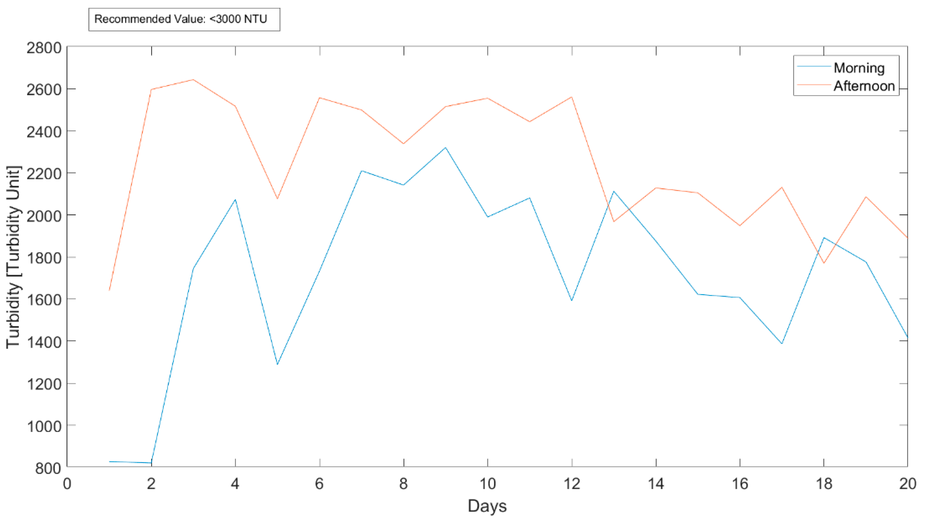
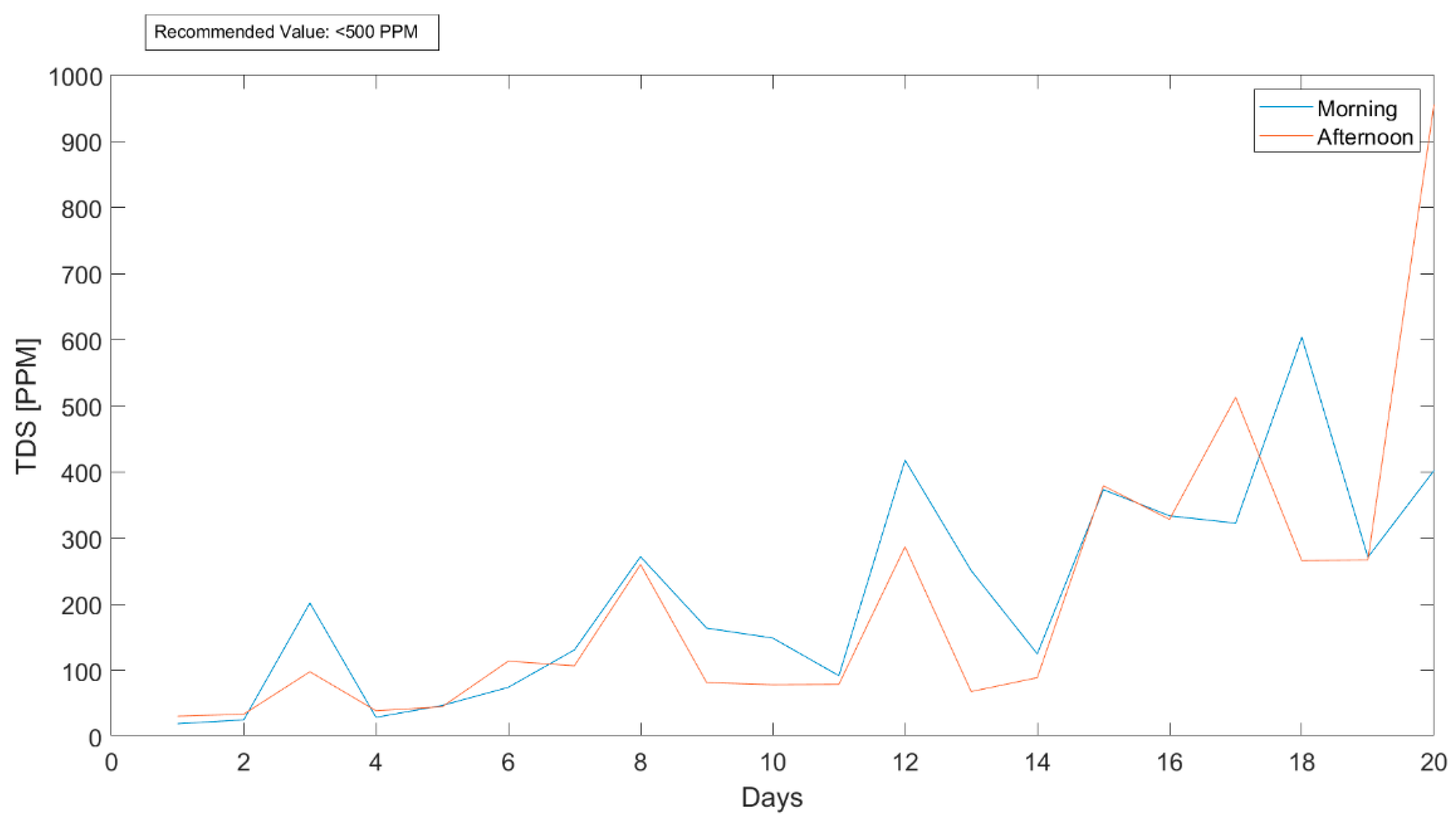
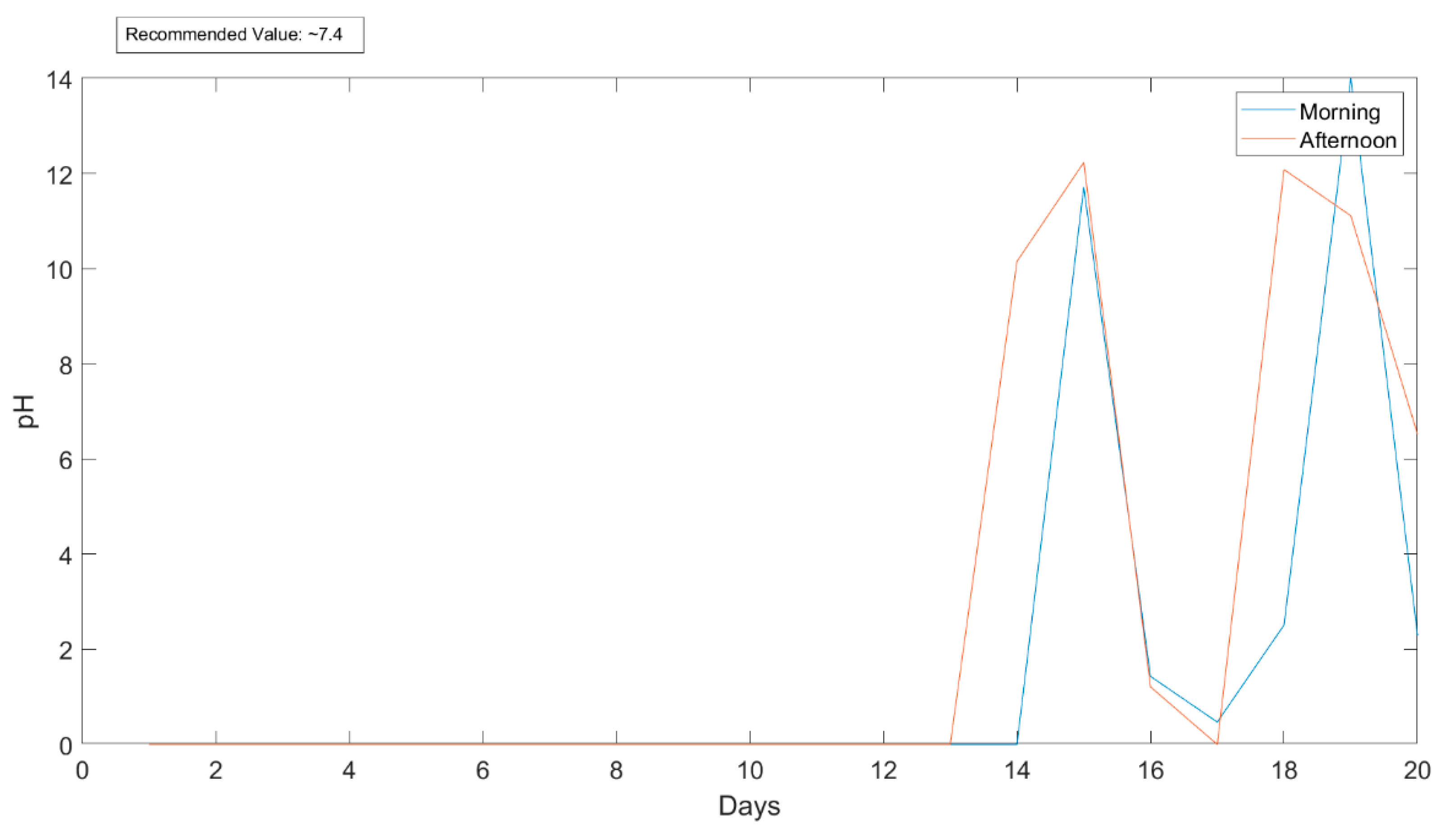
| Date | Time | Temperature (°C) | Turbidity (V) | Turbidity (NTU) | Total Dissolved Solids (PPM) | pH (V) | pH | |
|---|---|---|---|---|---|---|---|---|
| Week 1 | 7 October2019 | 10:30 am | 26.55 | 3.06 | 827.43 | 19.4 | - | - |
| Monday | 4:30 pm | 27.73 | 2 | 1639.13 | 30.8 | - | - | |
| 8 October 2019 | 10:10 am | 25.89 | 3.06 | 820.54 | 25.2 | - | - | |
| Tuesday | 4.10 pm | 27.56 | 0.75 | 2596.45 | 33.8 | - | - | |
| 9 October 2019 | 10:30 am | 25.92 | 1.86 | 1744.9 | 202 | - | - | |
| Wednesday | 4.00 pm | 27.67 | 0.69 | 2643.2 | 98 | - | - | |
| 10 October 2019 | 10:40 am | 25.35 | 1.43 | 2073.71 | 29 | - | - | |
| Thursday | 4.00 pm | 26.81 | 0.85 | 2516.73 | 39 | - | - | |
| 12 October 2019 | 9:50 am | 25.87 | 2.45 | 1288.85 | 47 | - | - | |
| Saturday | 3:50 pm | 27.12 | 1.43 | 2076.78 | 45 | - | - | |
| Week 2 | 14 October 2019 | 10:20 am | 25.92 | 1.87 | 1732.64 | 74.4 | - | - |
| Monday | 4:10 pm | 27.63 | 0.8 | 2557.36 | 114 | - | - | |
| 15 October 2019 | 10:00 am | 25.96 | 1.25 | 2210.15 | 131 | - | - | |
| Tuesday | 4:10 pm | 27.7 | 0.87 | 2499.11 | 107 | - | - | |
| 16 October 2019 | 10:30 am | 26.34 | 1.34 | 2141.93 | 272 | - | - | |
| Wednesday | 4:00 pm | 27.51 | 1.08 | 2338.15 | 260 | - | - | |
| 17 October 2019 | 10:20 am | 26.38 | 1.11 | 2320.52 | 164 | - | - | |
| Thursday | 4:10 pm | 27.3 | 0.85 | 2515.2 | 81.6 | - | - | |
| 19 October 2019 | 10:10 am | 26.75 | 1.54 | 1990.17 | 148.9 | - | - | |
| Saturday | 4:00 pm | 27.84 | 0.8 | 2555.06 | 78.4 | - | - | |
| Week 3 | 21 October 2019 | 10:50 am | 26.78 | 1.42 | 2080.61 | 92 | - | - |
| Monday | 3:50 pm | 28.23 | 0.95 | 2443.15 | 79 | - | - | |
| 22 October 2019 | 10:00 am | 26.84 | 2.06 | 1591.6 | 418 | - | - | |
| Tuesday | 4:10 pm | 28.21 | 0.79 | 2561.19 | 287 | - | - | |
| 23 October 2019 | 10:10 am | 24.28 | 1.38 | 2112.8 | 251 | - | - | |
| Wednesday | 4:00 pm | 25.59 | 1.57 | 1967.94 | 68 | - | - | |
| 24 October 2019 | 10:50 am | 25.26 | 1.69 | 1875.97 | 125 | - | - | |
| Thursday | 4:30 pm | 26.88 | 1.36 | 2128.13 | 89 | 2.2 | 10.15 | |
| 26 October 2019 | 12:30 pm | 26.84 | 2.02 | 1622.26 | 373.4 | 1.99 | 11.71 | |
| Saturday | 6:20 pm | 27.27 | 1.39 | 2105.14 | 379.2 | 1.92 | 12.23 | |
| Week 4 | 28 October 2019 | 10:20 am | 26.3 | 2.04 | 1606.93 | 333.8 | 3.39 | 1.43 |
| Monday | 3:20 pm | 26.47 | 1.59 | 1948.78 | 328.4 | 3.42 | 1.21 | |
| 29 October 2019 | 11:00 am | 25.27 | 2.33 | 1386.96 | 322.7 | 3.52 | 0.47 | |
| Tuesday | 4:30 pm | 26.16 | 1.35 | 2131.2 | 513 | 3.58 | 0 | |
| 30 October 2019 | 9:10 am | 25.27 | 1.67 | 1892.06 | 604 | 3.24 | 2.51 | |
| Wednesday | 4:10 pm | 26 | 1.83 | 1770.19 | 266 | 1.94 | 12.08 | |
| 1 November 2019 | 10:50 am | 25.88 | 1.82 | 1776.32 | 271.2 | 1.67 | 14 | |
| Thursday | 3:00 pm | 26.31 | 1.41 | 2086.74 | 267 | 2.07 | 11.11 | |
| 3 November 2019 | 11:30 am | 24.39 | 2.29 | 1414.55 | 402.4 | 3.27 | 2.29 | |
| Saturday | 4:30 pm | 25.01 | 1.67 | 1889 | 956.3 | 2.69 | 6.52 |
| Temperature | Turbidity | TDS | pH | |
|---|---|---|---|---|
| Average | 26.48 | 1986.99 | 210.67 | 6.59 |
| Minimum | 24.28 | 820.54 | 19.40 | 0.00 |
| Maximum | 28.23 | 2643.2 | 956.30 | 14.00 |
| Standard Deviation | 0.98 | 444.56 | 188.75 | 5.17 |
Publisher’s Note: MDPI stays neutral with regard to jurisdictional claims in published maps and institutional affiliations. |
© 2021 by the authors. Licensee MDPI, Basel, Switzerland. This article is an open access article distributed under the terms and conditions of the Creative Commons Attribution (CC BY) license (http://creativecommons.org/licenses/by/4.0/).
Share and Cite
Hong, W.J.; Shamsuddin, N.; Abas, E.; Apong, R.A.; Masri, Z.; Suhaimi, H.; Gödeke, S.H.; Noh, M.N.A. Water Quality Monitoring with Arduino Based Sensors. Environments 2021, 8, 6. https://0-doi-org.brum.beds.ac.uk/10.3390/environments8010006
Hong WJ, Shamsuddin N, Abas E, Apong RA, Masri Z, Suhaimi H, Gödeke SH, Noh MNA. Water Quality Monitoring with Arduino Based Sensors. Environments. 2021; 8(1):6. https://0-doi-org.brum.beds.ac.uk/10.3390/environments8010006
Chicago/Turabian StyleHong, Wong Jun, Norazanita Shamsuddin, Emeroylariffion Abas, Rosyzie Anna Apong, Zarifi Masri, Hazwani Suhaimi, Stefan Herwig Gödeke, and Muhammad Nafi Aqmal Noh. 2021. "Water Quality Monitoring with Arduino Based Sensors" Environments 8, no. 1: 6. https://0-doi-org.brum.beds.ac.uk/10.3390/environments8010006