Design of Machine Learning Prediction System Based on the Internet of Things Framework for Monitoring Fine PM Concentrations

Abstract

In this study, a mobile air pollution sensing unit based on the Internet of Things framework was designed for monitoring the concentration of fine particulate matter in three urban areas. This unit was developed using the NodeMCU-32S microcontroller, PMS5003-G5 (particulate matter sensing module), and Ublox NEO-6M V2 (GPS positioning module). The sensing unit transmits data of the particulate matter concentration and coordinates of a polluted location to the backend server through 3G and 4G telecommunication networks for data collection. This system will complement the government’s PM2.5 data acquisition system. Mobile monitoring stations meet the air pollution monitoring needs of some areas that require special observation. For example, an AIoT development system will be installed. At intersections with intensive traffic, it can be used as a reference for government transportation departments or environmental inspection departments for environmental quality monitoring or evacuation of traffic flow. Furthermore, the particulate matter distributions in three areas, namely Xinzhuang, Sanchong, and Luzhou Districts, which are all in New Taipei City of Taiwan, were estimated using machine learning models, the data of stationary monitoring stations, and the measurements of the mobile sensing system proposed in this study. Four types of learning models were trained, namely the decision tree, random forest, multilayer perceptron, and radial basis function neural network, and their prediction results were evaluated. The root mean square error was used as the performance indicator, and the learning results indicate that the random forest model outperforms the other models for both the training and testing sets. To examine the generalizability of the learning models, the models were verified in relation to data measured on three days: 15 February, 28 February, and 1 March 2019. A comparison between the model predicted and the measured data indicates that the random forest model provides the most stable and accurate prediction values and could clearly present the distribution of highly polluted areas. The results of these models are visualized in the form of maps by using a web application. The maps allow users to understand the distribution of polluted areas intuitively.

1. Introduction

Air pollution is the byproduct of human activities. However, the traditional method of collection fails to classify the pollution and cannot produce objective results. Many scientists are focused on the study of air pollution monitoring. El Fazziki et al. proposed an analytical system of pollution that is based on road infrastructure. This system was designed by using road networks in cities with Hadoop operation and the Dikstra algorithm to predict the real time air pollution of different road sections. Hu et al. [1] proposed a model for predicting the concentration of carbon monoxide. In the aforementioned study, the data of static and mobile monitoring systems could be used to predict and analyze CO concentration of the city of Sydney. The results of air pollution distribution of Sydney were visualized with a web application [2]. Kadri et al. proposed a distributed air pollution monitoring system based on solar power supply. This system transmits real time pollution information through webpages and mobile applications [3]. Mead et al. stated that air pollution monitoring for urban areas must be conducted at suitable spatial and temporal scales to facilitate the monitoring of the complicated environment. To address problems concerning the spatial scale, the aforementioned authors designed a microscale and low-cost gas sensor [4]. Predić et al. proposed the utilization of smart equipment to simplify monitoring. They used smart phones to construct an integrated platform for the wireless sensing of air quality (Exposure Sense). This platform, enabling third party sensing devices to be connected easily through a standard USB port, provides customized pollution data and uploads data to global sensor networks regularly [5]. On other hand, Shaban et al. proposed the construction of air pollution models by using a support vector machine, M5 pruned model tree, and artificial neural network. Multistep forecasting of urban air pollution was conducted, and the future concentrations of SO₂, NO₂, and O₃ were predicted [6]. Hasenfrate et al. proposed the construction of high resolution pollution maps by using a land use regression model. They installed wireless sensor nodes on trams in Zürich in order to solve the problem of the spatial variation of ultrafine particles [7]. Bacco et al. proposed an air pollution monitoring network based on information and communications technology. The network consists of stationary and mobile sensor nodes, and data collection is conducted with unmanned aerial vehicles. Incorporating a mobile social network application through which people express their subjective feelings, this network collects both objective data (sensors) and subjective feelings (people’s perception) simultaneously [8].

Chen et al. designed an anomaly detection framework for the supervision of sensor states and the determination of equipment malfunction. With this framework, the sensor maintenance operation can be conducted as soon as possible to ensure the credibility of the sensor data [9]. Singh et al. proposed the reconstruction of air pollution graphs by using the cokriging method. They analyzed the ozone and PM10 concentrations in an urban area in Northern Italy. Seasonal prediction, which the kriging interpolation method failed to complete, was achieved by using the cokriging method [10]. Sivaraman et al. proposed a low-cost mobile sensing unit that involved installing sensing equipment on cars and transmitted data to the back end in the form of a Google map through the 3G network. Sivaraman et al. used the aforementioned system to perform large range air pollution analysis of the Sydney metropolis [11]. Qu et al. proposed a comprehensive weather data visualization system that incorporates circular pixel bar charts embedded into polar systems, parallel coordinates, and weighted complete graphs. This proposed system was used to analyze air pollution problems in Hong Kong and specifically to reveal the correlations between wind direction, wind speed, and pollution [12]. Gu et al. developed a recurrent air quality predictor. By using key weather data and pollution values to determine the air pollutant concentration, the predictor predicts air quality several hours ahead, thus eliminating nonlinear and chaotic interference and resolving the problem of decreasing correlation with time [13]. Boubrima et al. deployed a low-cost wireless sensor network to design a model and to estimate sensor installation positions, achieving a sensor network with fine spatiotemporal granularity [14]. Al-Ali et al. used an online general packet radio service sensor array applied in air pollution monitoring to establish a personal application server with Internet connection, which was then tested in an urban area [15]. Chen et al. proposed a real time air pollution forecasting system. This system reduced the hardware cost to 10% of the original cost through the application of the Internet of Things (IoT) and predicted air pollution trends within a certain time range through neural network training [16]. Dam et al. proposed a wearable air quality monitor for air pollution analysis in different environments. This monitor can surmount the shortcomings of traditional distributed air pollution monitoring [17]. Qin et al. proposed a PM2.5 prediction system based on two deep neural networks, namely long short term memory and convolutional neural networks, to perform time series forecasting of the changes in the PM2.5 concentration [18]. Duangsuwan et al. proposed an air quality monitoring method based on NB-IoT, which involved using a sensing system comprising a low power wide area network for the real time monitoring of PM10, CO, CO₂, and O₃ concentrations and noise [19].

PM2.5 concentration changes with time and area. In the present study, monitoring was performed using the Taiwanese government’s regional monitoring stations and mobile sensing devices. The regional monitoring stations provide continuous high stability and high accuracy pollutant concentration monitoring data. However, only limited regional monitoring stations have been set up due to their high cost. Mobile sensing devices facilitate detailed monitoring in each area, have the advantages of low cost and portability, and can be installed on streets. However, these devices are relatively unstable and prone to incomplete data collection. Built on the IoT framework, this study capitalized on the advantages of both mobile sensing devices and regional monitoring stations for pollutant concentration prediction. Machine learning models were used to design a prediction system for the PM2.5 concentration in urban areas. Changes in the PM2.5 concentration in urban areas were predicted in real time, and pollution distribution maps were then generated using a web application. To sum up these studies mentioned above, combining the Internet of Things framework and machine learning is the novel idea for our further study.

Metropolitan areas are densely populated areas where the quality of air has a direct impact on health. Until now, air pollution monitoring in metropolitan areas has mainly been carried out by government agencies through the installation of fixed monitoring stations. Although these stations are highly accurate, they are expensive to install and occupy large space. As a result, the number of stations is sparse, and the distances between them are generally far apart, making it difficult to estimate the true pollution value of a particular area. In order to monitor fine particulate pollution more accurately, this research proposes a metropolitan area fine particulate prediction system based on the Internet of Things (IoT) and combined with a machine learning model.

2. Problem Statements

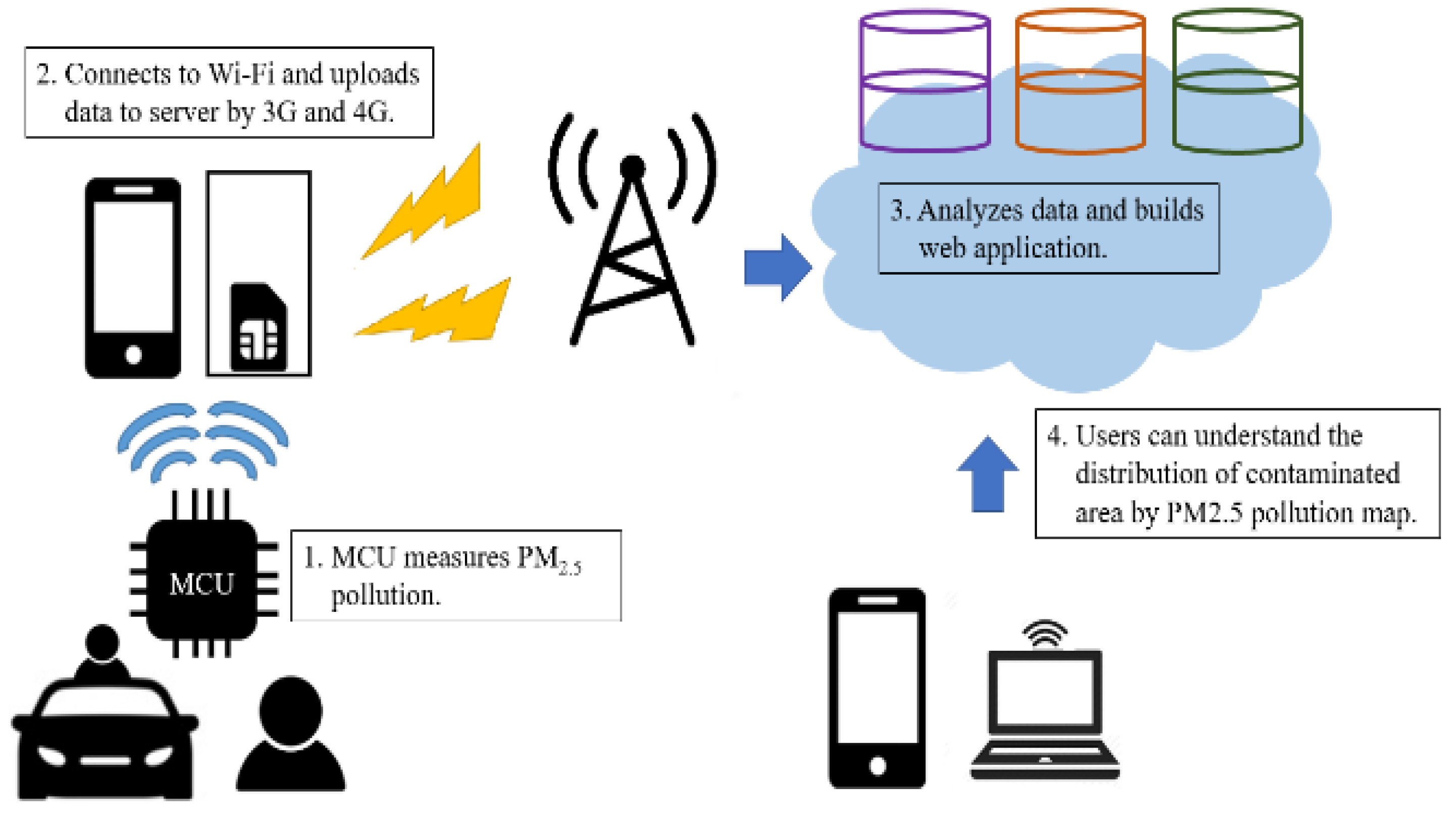
2.1. System Architectures

The structure of the system used in this study is displayed in Figure 1. This system consists of four parts: an environment sensing unit, a wireless transmission channel, a cloud database, and a web application.

The environment sensing unit is composed of the Chnia, Ai-Thinker, NodeMCU-32S microcontroller, a Switzerland, Ublox, GPS neo-6M V2 positioning module, a China, PLANTOWER, PMS5003 G5 PM sensing module, a power bank, and Internet connection equipment. Figure 2 depicts the hardware equipment. To prevent the environment sensing unit from being damaged by wind or rain, a double layer case design was adopted. The case is displayed in Figure 3. Figure 4 illustrates the process of the environment sensing, and the time interval between each data upload is 5 s.

Cell sites in Taiwan have extremely high distribution density and are managed by government agencies at all times. Thus, a telecommunication network, comprising cell sites, provides high coverage, stable transmission, and high reliability. After the sensors collect environment data, the system enters the wireless transmission stage. Subsequently, the Chnia, Ai-Thinker, NodeMCU-32S microcontroller communicates with the Internet connection equipment through Wi-Fi, connects to the 3G or 4G telecommunication network through a subscriber identity module (SIM) card, and sends the environment data to the backend database for storage.

The backend database system is constructed by using California, USA, ORACLE, MySQL, which is a relational database management system, and the XAMPP software package developed by Kai ‘Oswald’ Seidler and Kay Vogelgesang. XAMPP allows users to construct web servers on personal computers and manage the database. The environment data are stored in MySQL, and California, USA, ORACLE, SQL grammar and PHP grammar founded by Rasmus Lerdorf are used to access the data for organization and analysis.

The web application was constructed using the Apache HTTP server developed by Apache foundation and interacts with users through Leaflet, which is a frontend map package. Leaflet has the characteristics required by most map systems. It can switch between satellite cloud images and street maps according to users’ needs. The lightweight nature of Leaflet reduces the running load. Users can inquire the pollution distribution locations through webpages to understand PM pollution. Figure 5 displays the heat distribution in Leaflet.

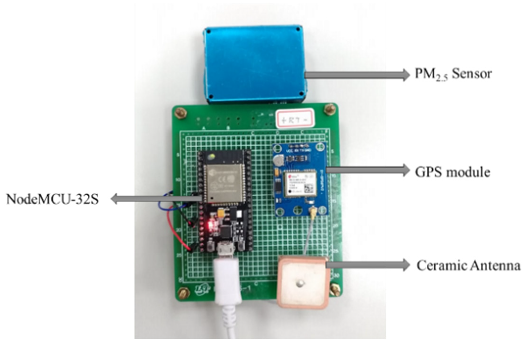
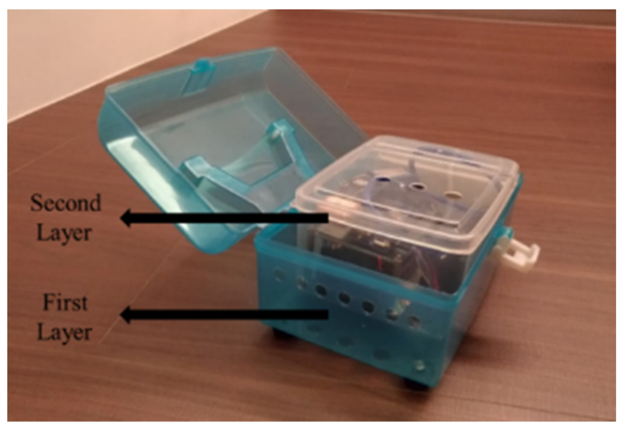
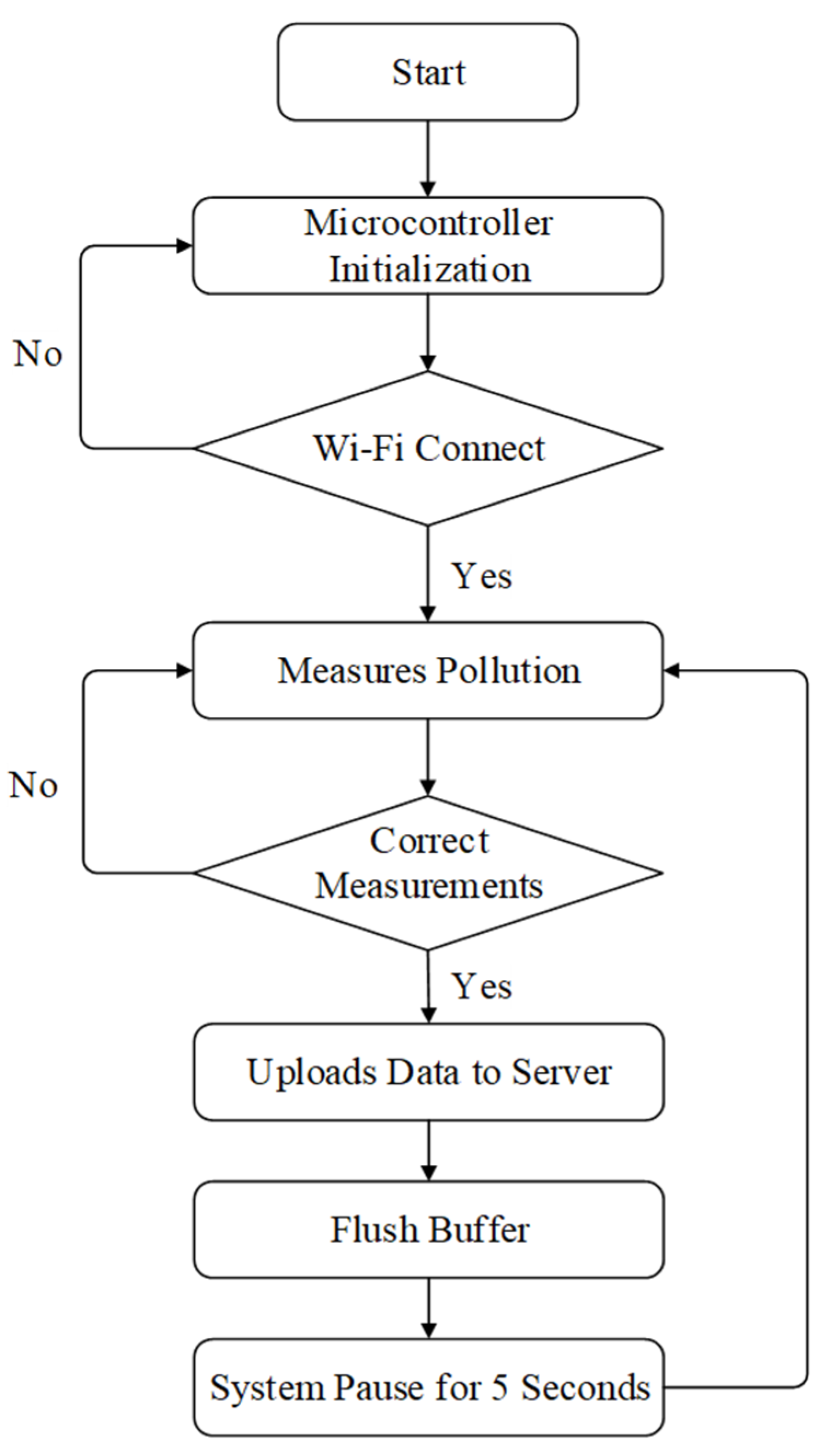
2.2. IoT for Fine Suspended Particulate Monitoring

The pollution of fine suspended particulates is an issue of increasing concern to all countries, and we hope to mitigate the pollution situation in the course of economic development. The monitoring of PM2.5 pollution is usually carried out by fixed monitoring stations set up by the government, mainly by the Environmental Protection Administration of the Executive Yuan in Taiwan. Large stationary monitoring stations are highly accurate and have excellent system stability. However, they are expensive to build, occupy large space, and are located far away from each other, which limits the number of stations. For example, the Taipei metropolitan area covers an area of 2457.1253 km² and has a population of 7,032,434, but there are only 20 large monitoring stations, so it is difficult to directly reflect the true pollution level. Figure 6 (cited from the Environmental Protection Administration, Executive Yuan) shows the distribution of fixed monitoring stations in the Taipei metropolitan area.

Another way of monitoring PM2.5 is manual monitoring. The person in charge of sampling uses specially treated filter to collect at a specific point and sends the paper back to the laboratory for analysis. The advantage of manual monitoring is that it eliminates as many external environmental disturbances as possible and calculates the pollution value by weighing under controlled environmental conditions such as temperature and humidity. However, the entire process must go through a complete experimental analysis process and often takes two to three weeks to produce the final results, so it does not provide an early warning effect to the public.

With the booming development of single chip technology, environmental sensing technology and wireless transmission technology, the application of Internet of Things is becoming more and more mature. In recent years, a variety of portable mobile sensing devices have emerged one after another. The Edi Green Air Box is a three way cooperation platform between the private sector, research institutes, and the government and can be placed on public transportation for stable environmental data collection. Through the Internet of Things, the PM2.5 pollution values of the area can be obtained from the alleys and streets, which can compensate for the insufficient number of fixed monitoring stations and the time consuming nature of manual collection. However, the relative instability of mobile sensor system data sensing may also be due to external factors causing fragmented data. Both fixed stations and mobile sensors have their own advantages and disadvantages, and it is impossible to give too much weight to the data results of one or the other, so the best approach for PM2.5 pollution analysis is to use both methods.

3. Design of the PM Predictive System

3.1. PM Pollution Dataset

The dataset used in this study is the PM2.5 pollution dataset collected for three urban areas in Taiwan, namely Xinzhuang, Sanchong, and Cailiao Districts, from 13 December 2018, to 9 February 2019. The adopted dataset is a winter pollution dataset that contains 11,854 data points. The time interval between each data upload is 5 s, and the data sensor travels at a speed lower than 70 km/h. Accordingly, the distance between each measurement location is within 100 m. The data structure consists of seven types of information, namely pollutant measurement time (h), longitude, latitude, the pollutant concentration at Xinzhuang Station, the pollutant concentration at Sanchong Station, the pollutant concentration at Cailiao Station, and the pollutant concentration measured by the sensor. The sensing unit designed in this study was used to collect four types of data, namely data on longitude, latitude, pollutant measurement time, and pollutant concentration. The data of the stationary stations were obtained from the open database of the Taiwanese government.

Figure 7 displays the data recorded at 11:00 A.M. on 20 January 2019. In this figure, the horizontal axis represents the longitude and the vertical axis represents the latitude. The pollution level is depicted with the heat scale at the right side of Figure 7. The average PM2.5 value on the aforementioned day was 34 μg/m³. The road section at the upper left had high pollutant concentration; thus, it exhibits an orangish red color. Figure 8 depicts the data recorded at 10:00 A.M. on 3 January 2019. Most of the areas are in dark blue, which indicates that these areas had low pollution levels. Only few road sections had a marginally high pollutant concentration, which are indicated by a slight green color.

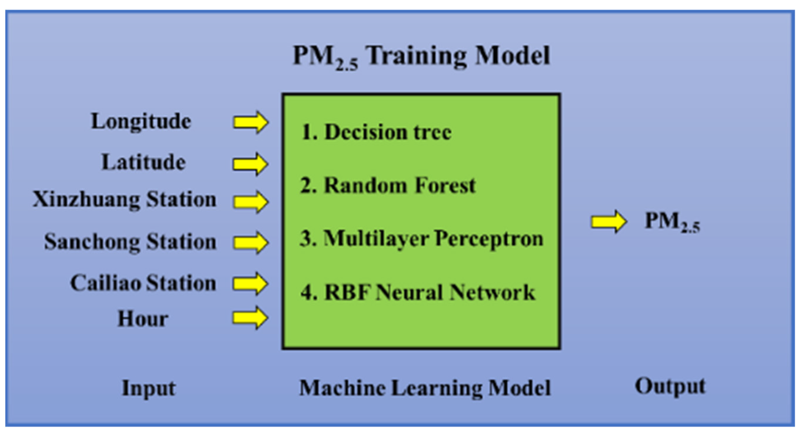
3.2. Structure of the Machine Learning Models

The proposed PM2.5 prediction model is displayed in Figure 9. The input features are six-dimensional data comprising information on longitude, latitude, the pollutant concentration at Xinzhuang Station, the pollutant concentration at Sanchong Station, the pollutant concentration at Cailiao Station, and pollutant measurement time (h). The pollutant concentrations at the aforementioned three stations reflected the overall pollution situation in the corresponding three metropolitan areas. The spatial and temporal input features of longitude, latitude, and pollutant measurement time were used to accurately describe the PM2.5 pollution level of each small region within the metropolitan areas. The model output is the PM2.5 value (μg/m³). Four types of machine learning models were used for training, namely decision tree, random forest, multilayer perceptron, and radial basis function (RBF) neural network.

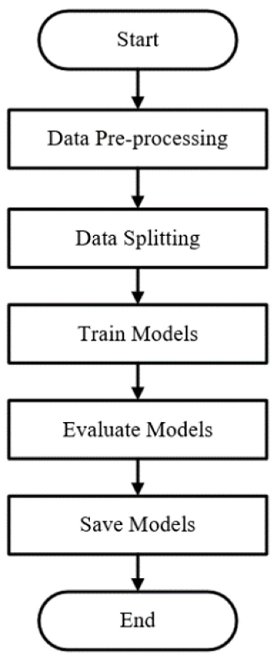
3.3. Model Training Process

Figure 10 displays the model training process adopted in this study. This process comprises five major steps.

3.3.1. Model Training Process

Missing data in the database were removed to prevent them from influencing the training process. Data outside the range of 0–100 μg/m³ were determined to be abnormal data and thus were also deleted. Feature scaling is conducted on the data to enhance the convergence likelihood of the model learning process. MinMaxScaler in scikit-learn was used for the feature scaling with the scaling ranges of 0 to 1 and −1 to 1. For the decision tree and random forest models, a feature scaling range of 0–1 was used. For the multilayer perceptron and RBF neural network models, a feature scaling range of −1 to 1 was used.

$$X_{std}=\frac{X-X_{min}}{X_{max}-X_{min}},$$

(1)

$$X_{minmax}=X_{std}\cdot \left(max-min\right)+mi{n}_{,}$$

(2)

where

$X$ is current value;

$X_{min}$ is minimum value of the same feature data;

$X_{max}$ is maximum value of the same feature data;

$max$ is maximum value of the feature scaling data;

$min$ is minimum value of the feature scaling data;

$X_{minmax}$ is value after feature scaling.

3.3.2. Data Grouping

The data were reshuffled to increase their randomness. In addition, 80% of the data were assigned to the training set, and the remaining 20% were assigned to the testing set. The training set comprised 9483 data points, and the testing set comprised 2371 data points.

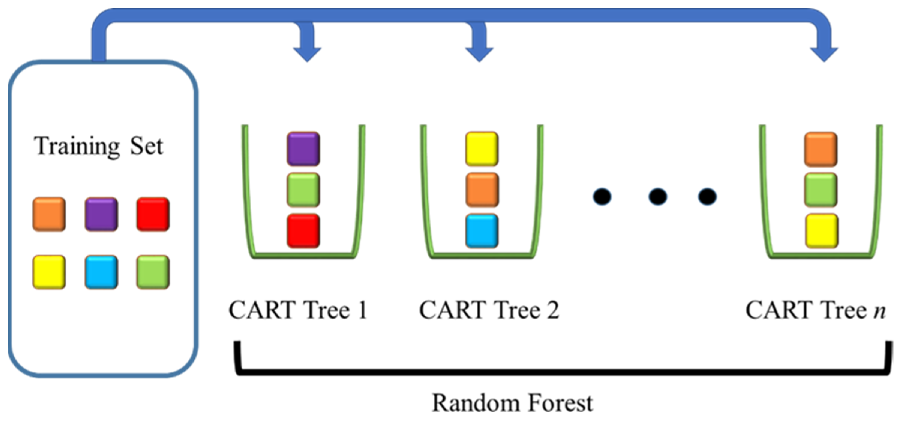
3.3.3. Machine Learning Methods

Machine learning adopts appropriate learning rules according to the different situations in which it is used. This study used the supervised learning method as the basis for urban pollution analysis. The following sections introduce the calculations of the classification and regression decision tree (CART), random forest, multilayer perceptron (MLP), and RBF network [20,21] methods.

In the CART regression algorithm used in this study, the decision tree uses the split method to grow from top to bottom, and in each step of the splitting process, the best attribute is selected for splitting so that the error value is reduced, as shown in Formula (3), where $x^{(j)}$ represents the selected feature, the feature value s is used as a reference point for splitting. The data space is cut into two regions $R_1(j,s)$, $R_2(j,s)$, and the output value $y_1$, $y_2$ of the region $R_1$, $R_2$ is the average value of the expected output of each region, E means the expectation operation, and t_i means the ith data,

$$R_1(j,s)=\left\{x|x^{(j)}\le s\right\},R_2(j,s)=\left\{x|x^{(j)}>s\right\},$$

(3)

$$y_1=E(t_i|x_i\in R_1(j,s){)}_{,}$$

(4)

$$y_2=E(t_i|x_i\in R_2(j,s){)}_{,}$$

(5)

The minimum square error of the CART regression algorithm is

$$min{\left[{\displaystyle \sum _{x_i\in R_1}{(t_i-y_1)}^2+{\displaystyle \sum _{x_i\in R_2}{(t_i-y_2)}^2}}\right]}_{,}$$

(6)

In the process of random forest training, multiple CARTs are combined for co-training, and multiple decision trees form a “forest” model, which can improve the prediction dead ends of a single decision tree model and can reduce the chance of overfitting. The model is shown in Figure 11. Random forest is different from traditional decision tree models for testing all features of the dataset. It does not directly search and test all features but randomly selects node features. Therefore, random forest increases the randomness of the model and reduces the tree.

The training process of the multilayer perceptron can be divided into two stages. In the first stage, the input variables are continuously fed forward to the output layer through the excitation between nodes, which is a standard feedforward neural network. In the second stage, the neural network model is trained, and the weights of the model are corrected one by one through backpropagation (BP) to find a suitable parameter so that the output of the network model can be made as close as possible to the expected value. . The error function is defined as shown in Equation (7)

$$error=\frac{1}{2}{{\displaystyle \sum _j{(T_j-Y_j)}^2}}_{,}$$

(7)

where $T_j$ represents the expected output of the jth neuron in the output layer, and $Y_j$ represents the output of the jth neuron network in the output layer.

The RBF neural network is different from the MLP in that its hidden layer uses a nonlinear radial basis function as a learning function. The Gaussian function is a commonly used RBF, and it is also an important core of the RBF neural network. The input variable is converted to the hidden layer through Gaussian function conversion. The closer the input variable of the neuron is to the center of the Gaussian function, the higher the level of excitation of the neuron, and vice versa. Conversely, the degree of excitation decreases rapidly.

3.3.4. Model Training

The learning models were established using Python programming in scikit-learn and TensorFlow. Scikit-learn exhibits abundant feature operations and provides an application programming interface for machine learning algorithms, facilitating the construction of learning models according to application requirements. The strength of TensorFlow is that it can be used for the construction of neural network models. Moreover, TensorFlow offers various reverse transmission methods. The decision tree, random forest, and multilayer perceptron models were constructed using scikit-learn, and the RBF neural network model was constructed using TensorFlow.

To reduce overfitting for the decision tree algorithm, the tree model growth was limited by adjusting the following parameters: max_depth (maximum depth of the tree structure), min_samples_split (sample size required for the splitting process), and splitter (splitting method). The random forest algorithm is a combination of multiple decision trees. The number of decision tress was controlled by adjusting n_estimators.

The four parameters set for the multilayer perceptron model are number of hidden layers, number of nodes in each layer, activation function, and optimizer. The number of hidden layers was set as 3, and the number of nodes in each layer was set as 29. The rectified linear activation function (ReLU) was used, and Adam Optimizer was used as the optimizer.

The two parameters set for the RBF neural network model were optimizer and number of nodes. The number of nodes was set as 120, and Adam Optimizer was adopted as the optimizer.

Table 1. Training parameters of the learning models.

Decision tree	max_depth	15
	min_samples_split	11
	splitter	Random
Random Forest	max_depth	15
	min_samples_split	11
	n_estimators	20
Multilayer Perceptron	Hidden Layers	3
	Nodes	29
	Activation Function	ReLU
	Optimizer	AdamOptimizer
RBF Neural Network	Nodes Optimizer	120 AdamOptimizer

presents the training parameter settings of the learning models.

3.4. Model Training Process

In this study, the root mean square error (RMSE) and mean absolute error (MAE) were used as indicators to assess the learning results.

$$RMES=\sqrt{\frac{{\sum }_{i-1}^n{e}_i^2}{n}}$$

(8)

$$MAE=\frac{{\sum }_{i=1}^n\left|e_i\right|}{n}$$

(9)

where e_i is the error between the model output and expected output and n is the total learning sample size.

3.5. Model Saving

The models were saved using the joblib tool in scikit-learn and the tf.train.Saver tool in TensorFlow.

4. Model Training Comparison

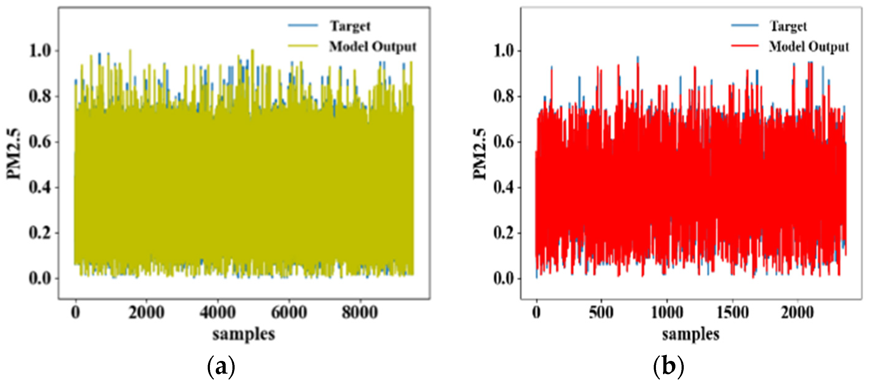
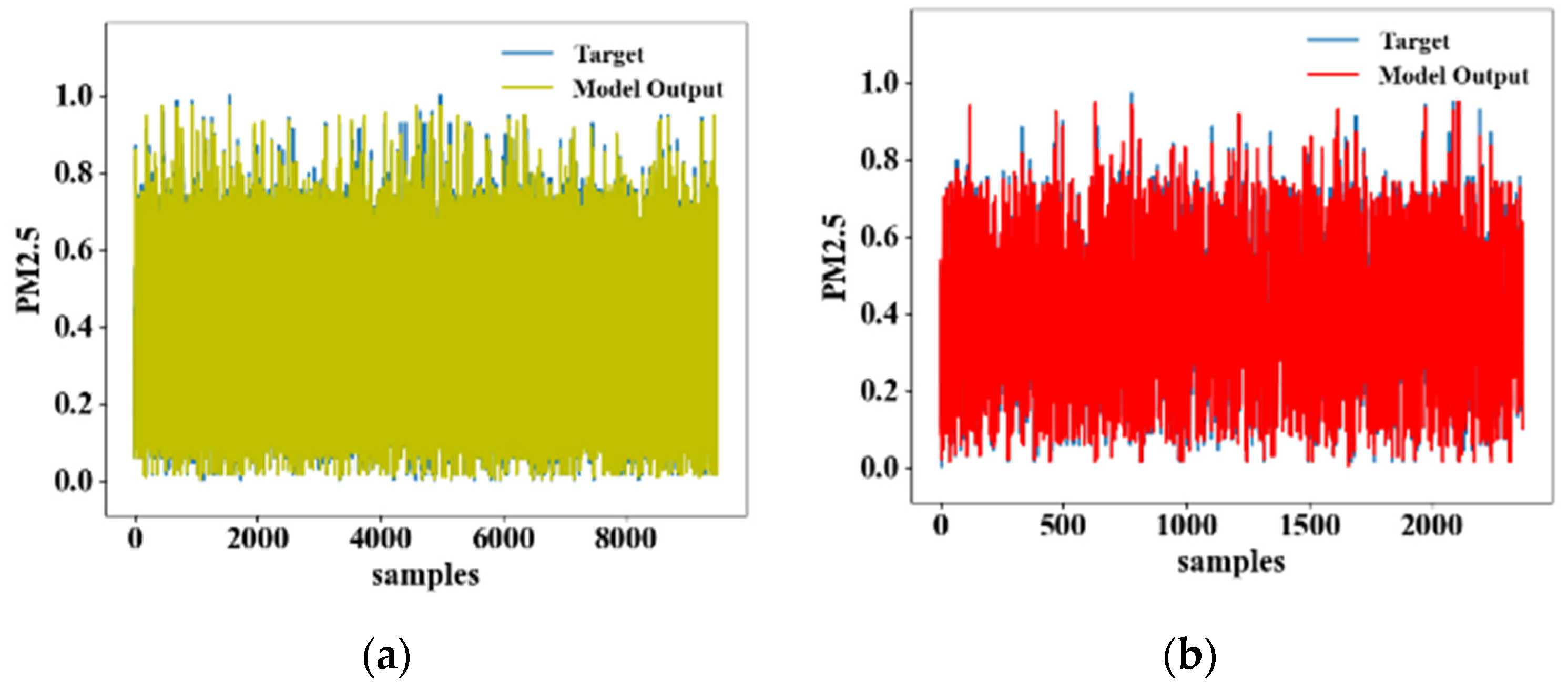
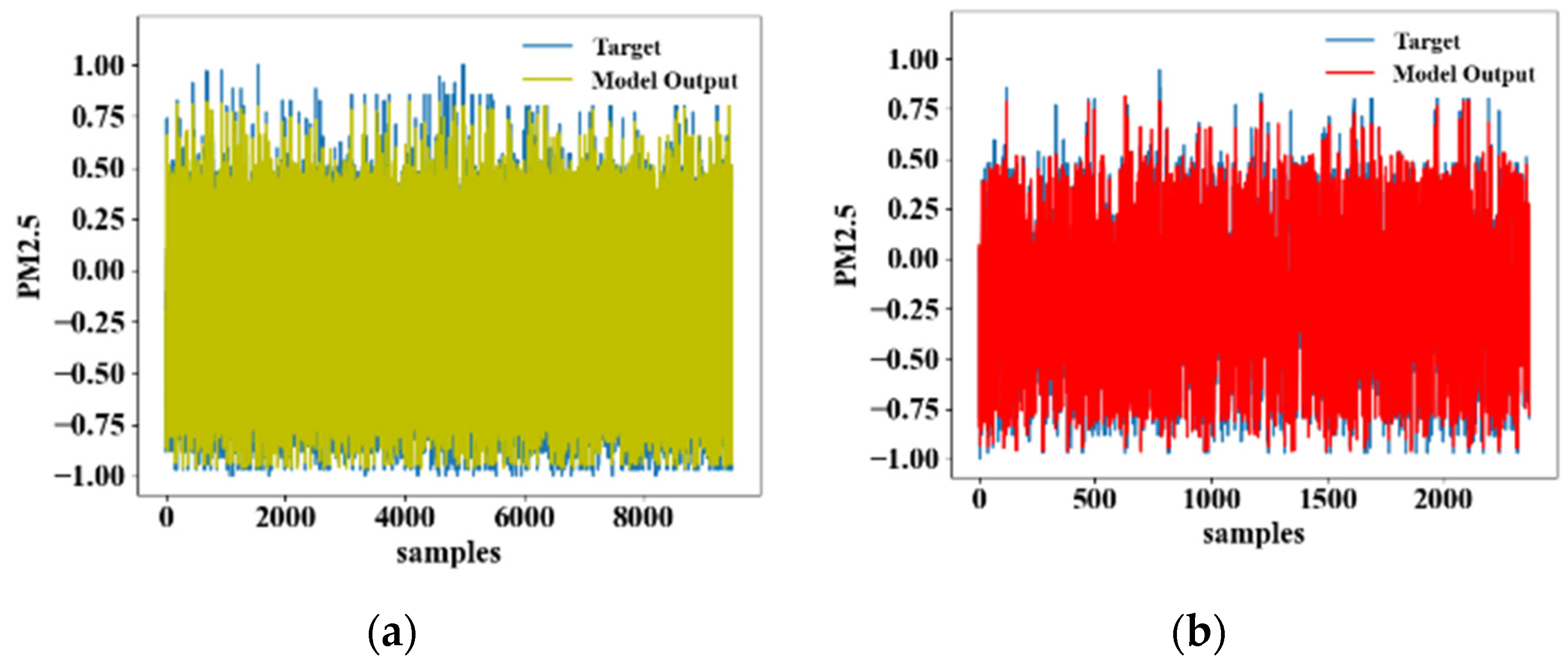
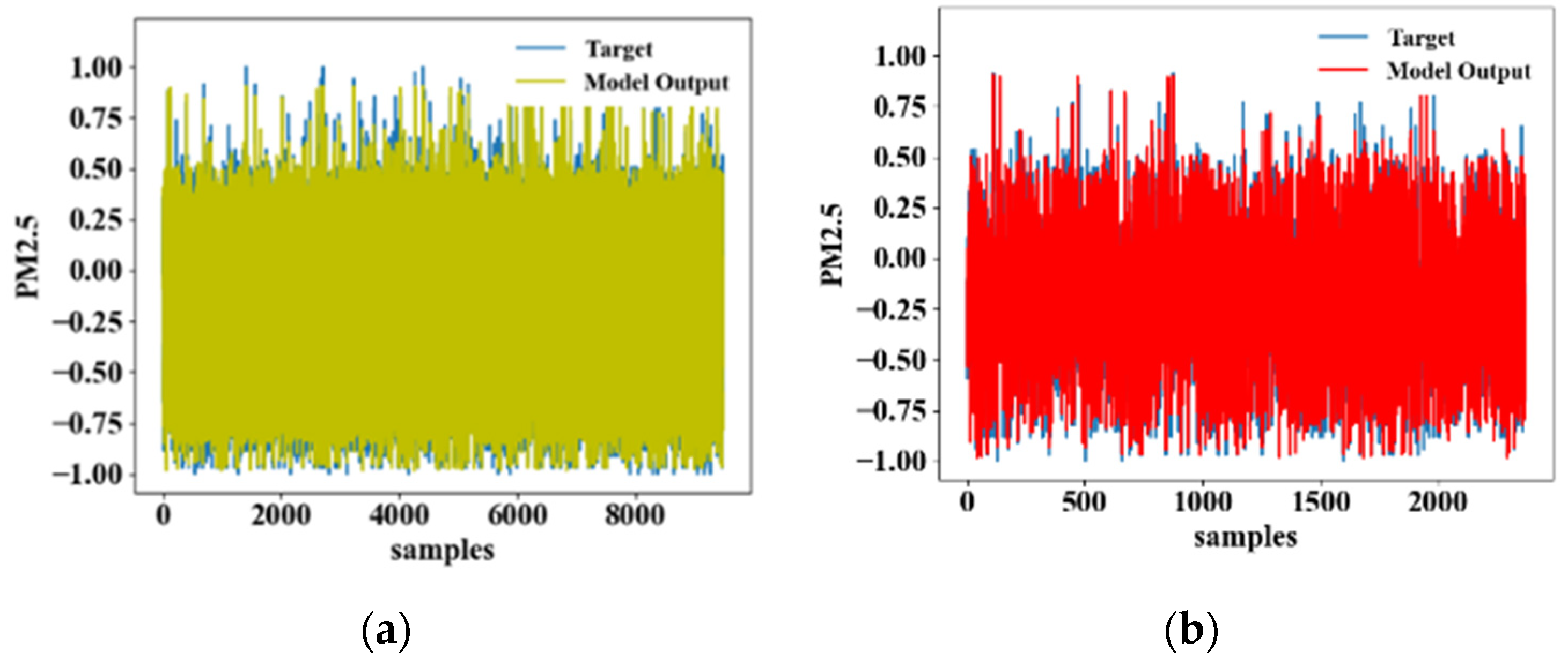
4.1. Comparison of the Model Learning Results

Figure 12, Figure 13, Figure 14 and Figure 15 display the learning results of the models.

Table 2. RMSE values of the four adopted learning models.

Model	Data Pre Processing	Training	Testing
Decision tree	MinMaxScaler (0~1)	0.0242	0.0296
Random forest	MinMaxScaler (0~1)	0.0168	0.0236
Multilayer perceptron	MinMaxScaler (−1~1)	0.0892	0.0899
RBF neural network	MinMaxScaler (−1~1)	0.0830	0.0872

presents the RMSE values of the four learning models. The feature scaling range of the decision tree model was 0–1. The RMSE values of the training and testing sets for the aforementioned model were 0.0242 and 0.0296, respectively. The learning results for the training and testing sets were similar, and no apparent overfitting or under fitting was observed. The feature scaling range of the random forest model was also 0 to 1. The RMSE values of the training and testing sets for the aforementioned model were 0.0168 and 0.0236, respectively. The random forest model exhibited the optimal results among all the models. The feature scaling range of the multilayer perceptron model was −1 to 1. The RMSE values of the training and testing sets for the aforementioned model were 0.0892 and 0.0899, respectively. The feature scaling range of the RBF neural network was also −1 to 1. The RMSE values of the training and testing sets for the aforementioned model were 0.0830 and 0.0872, respectively. The training and testing results were similar. The random forest model provided the best learning results, followed by the decision tree and RBF neural network models. The multilayer perceptron model exhibited the largest errors.

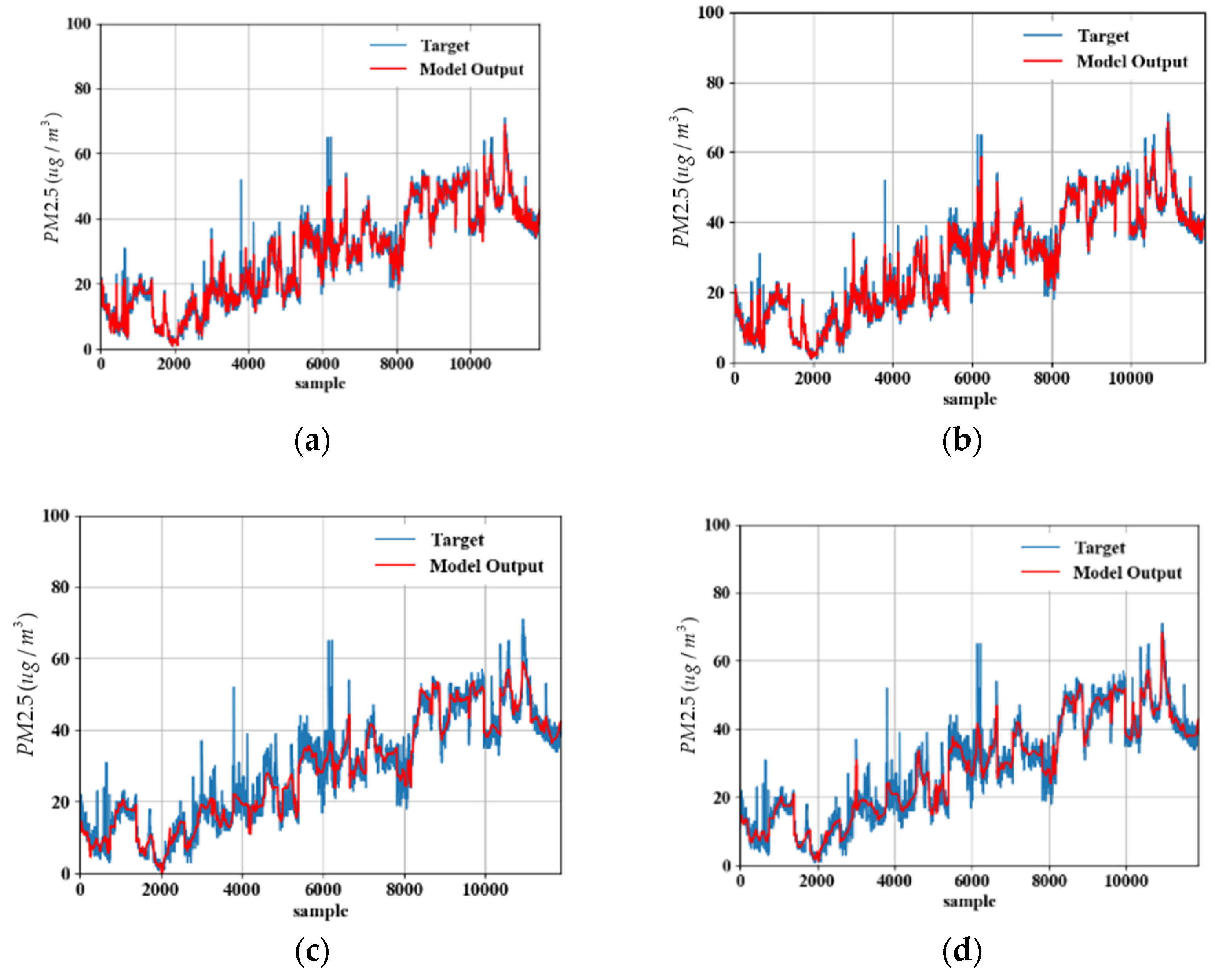
4.2. Comparison of the Model Output Results

Figure 16a–d show the errors between the output values of the four learning models and the measured pollutant concentrations. In the figures mentioned above, the Y-axis indicates the PM2.5 values (μg/m³), and the X-axis indicates the dataset sample size. The blue lines represent the real pollutant concentrations, and the red lines represent the model output values. The MAE is used to determine the errors. As displayed in Figure 16a–d, the overall MAEs of the decision tree, random forest, multilayer perceptron, and RBF neural network models were 1.0680, 0.8099, 2.2612, and 2.1642 μg/m³, respectively.

Table 3. MAE values of the learning models.

Model	MAE (μg/m3)
Decision tree	1.0680
Random forest	0.8099
Multilayer perceptron	2.2612
RBF neural network	2.1642

presents the MAE values of the models. The random forest model exhibited the optimal performance, followed by the decision tree, RBF neural network, and multilayer perceptron models.

This chapter introduces the proposed fine aerosol machine learning prediction system in detail and compares the learning effectiveness of the four learning models with the root mean square error and the average absolute error. The results show that tree structure models such as decision trees and random forest models can learn well for various input features and have better learning results. The random forest model further improves the learning effect of decision trees.

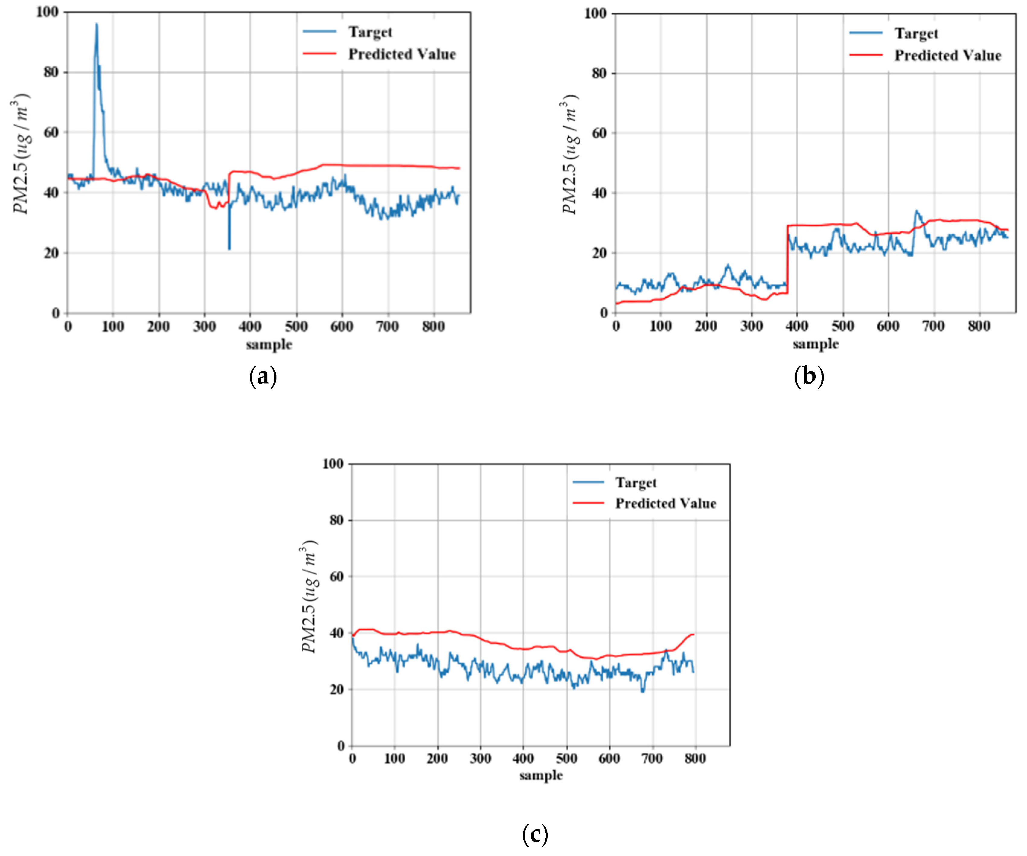
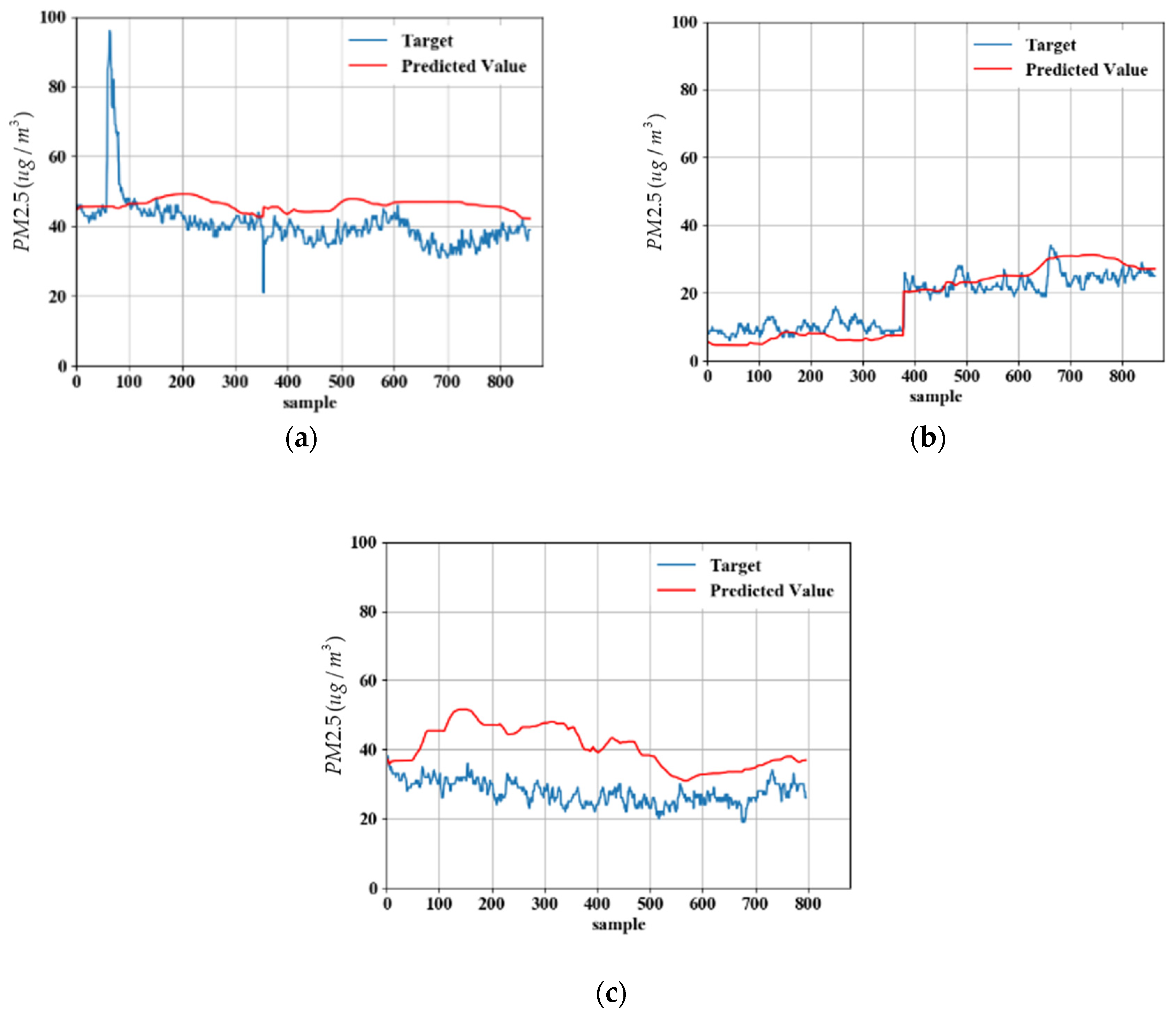
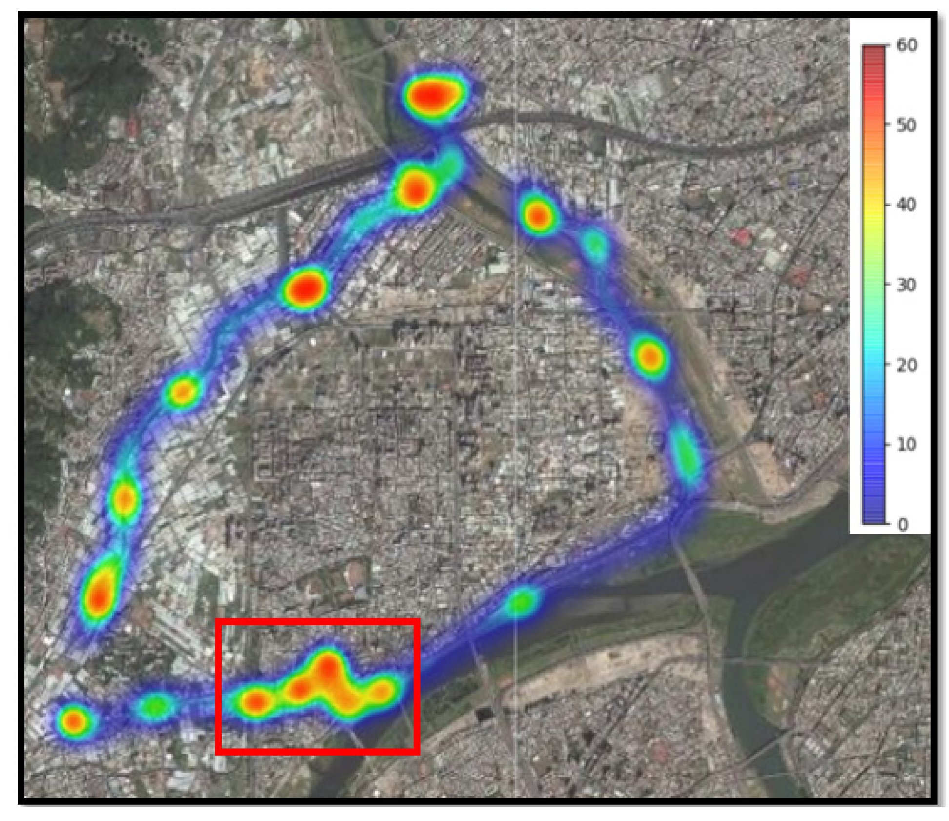
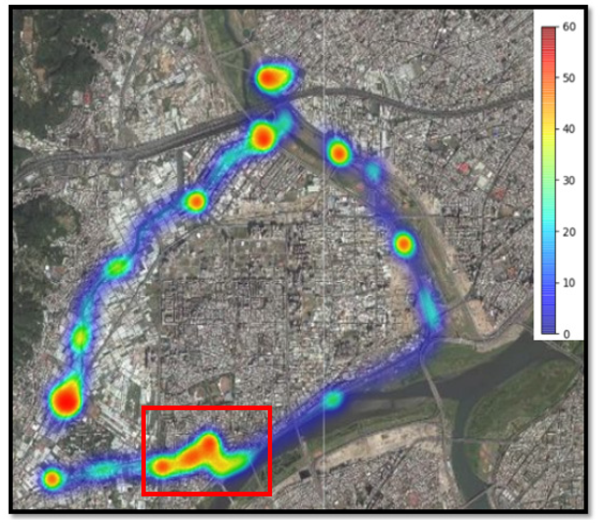
5. Experimental Results

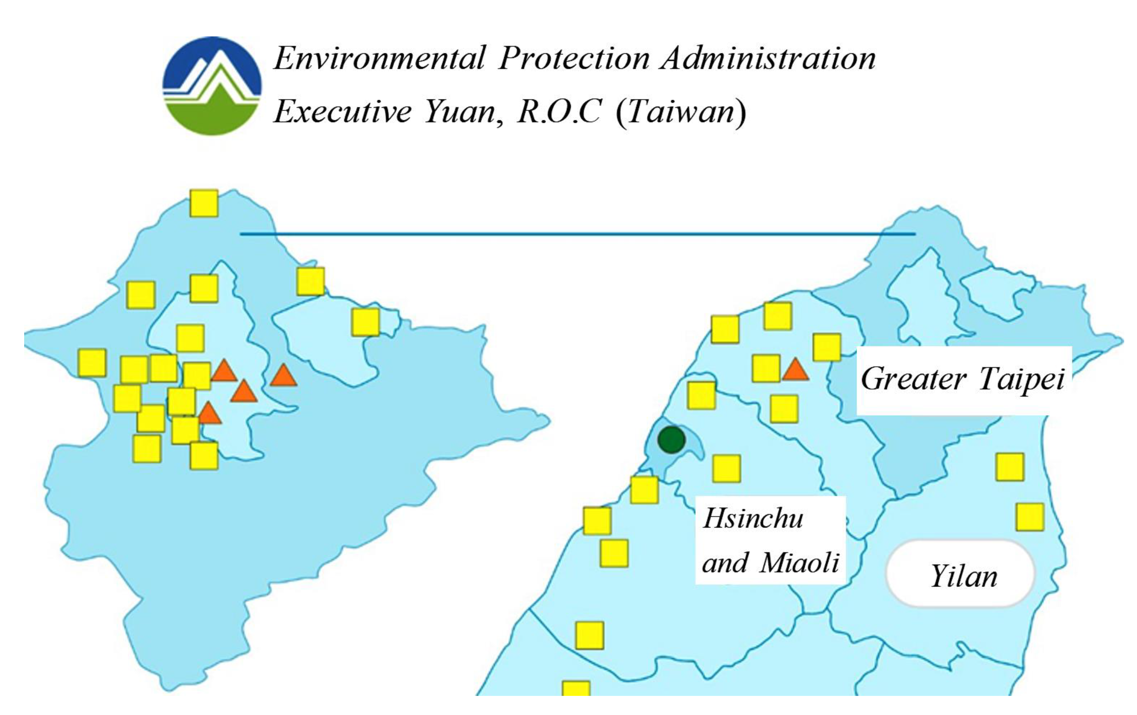
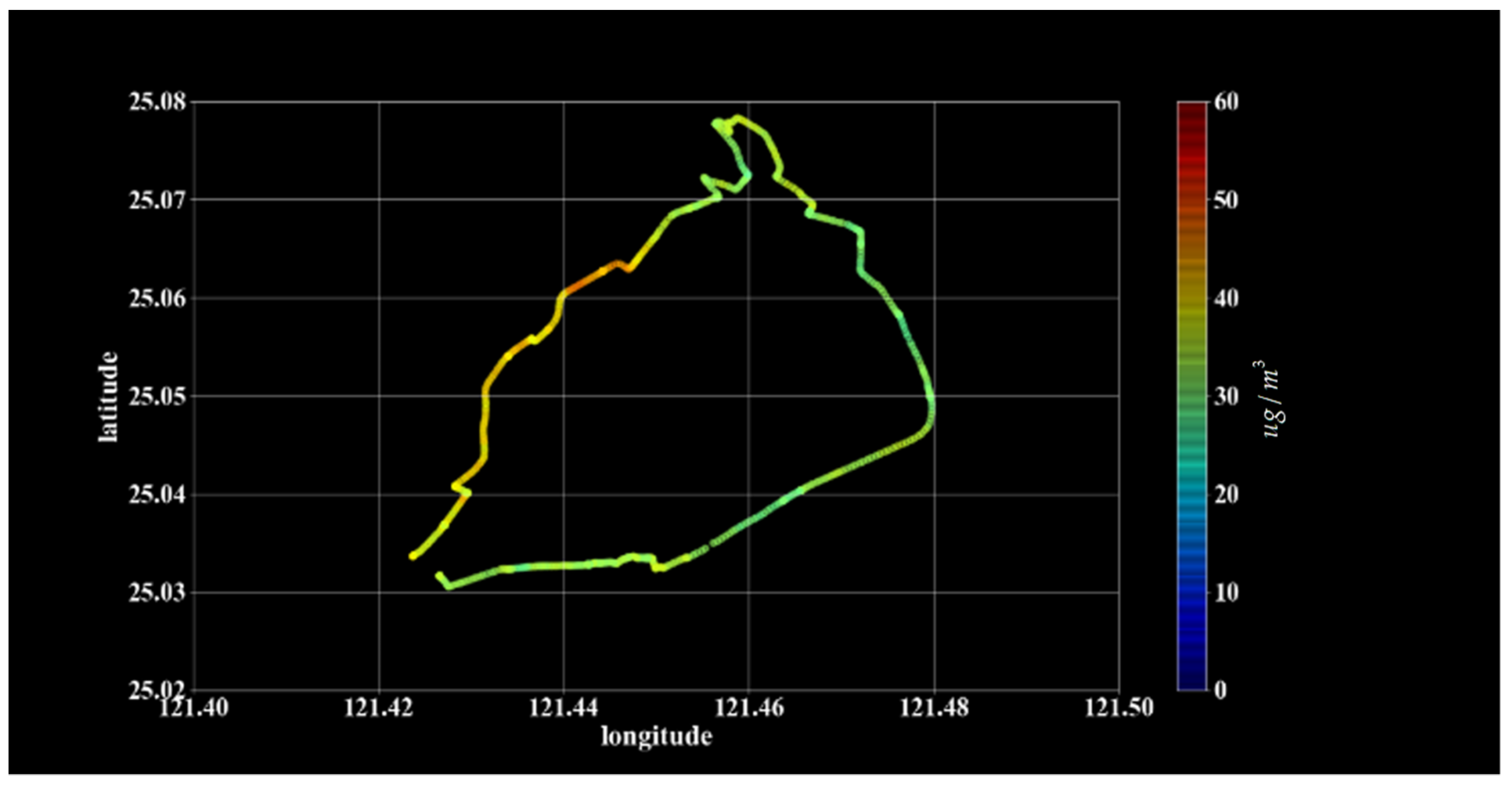
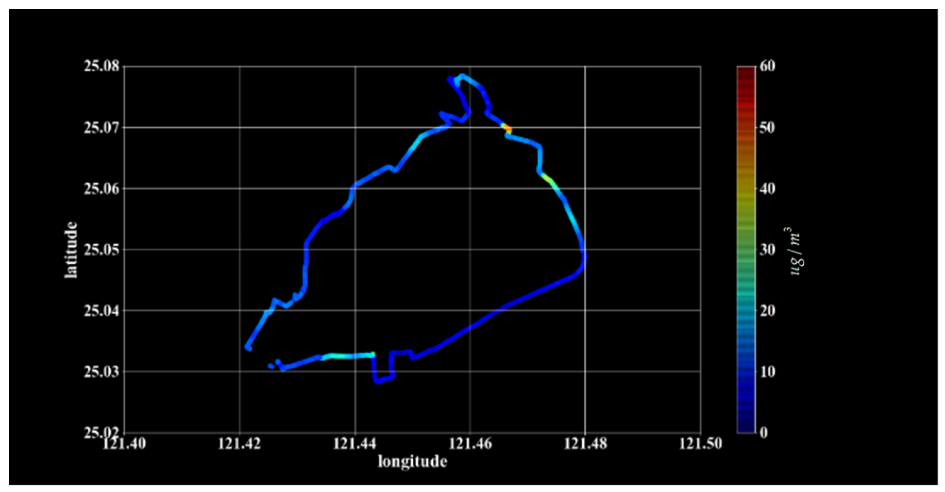
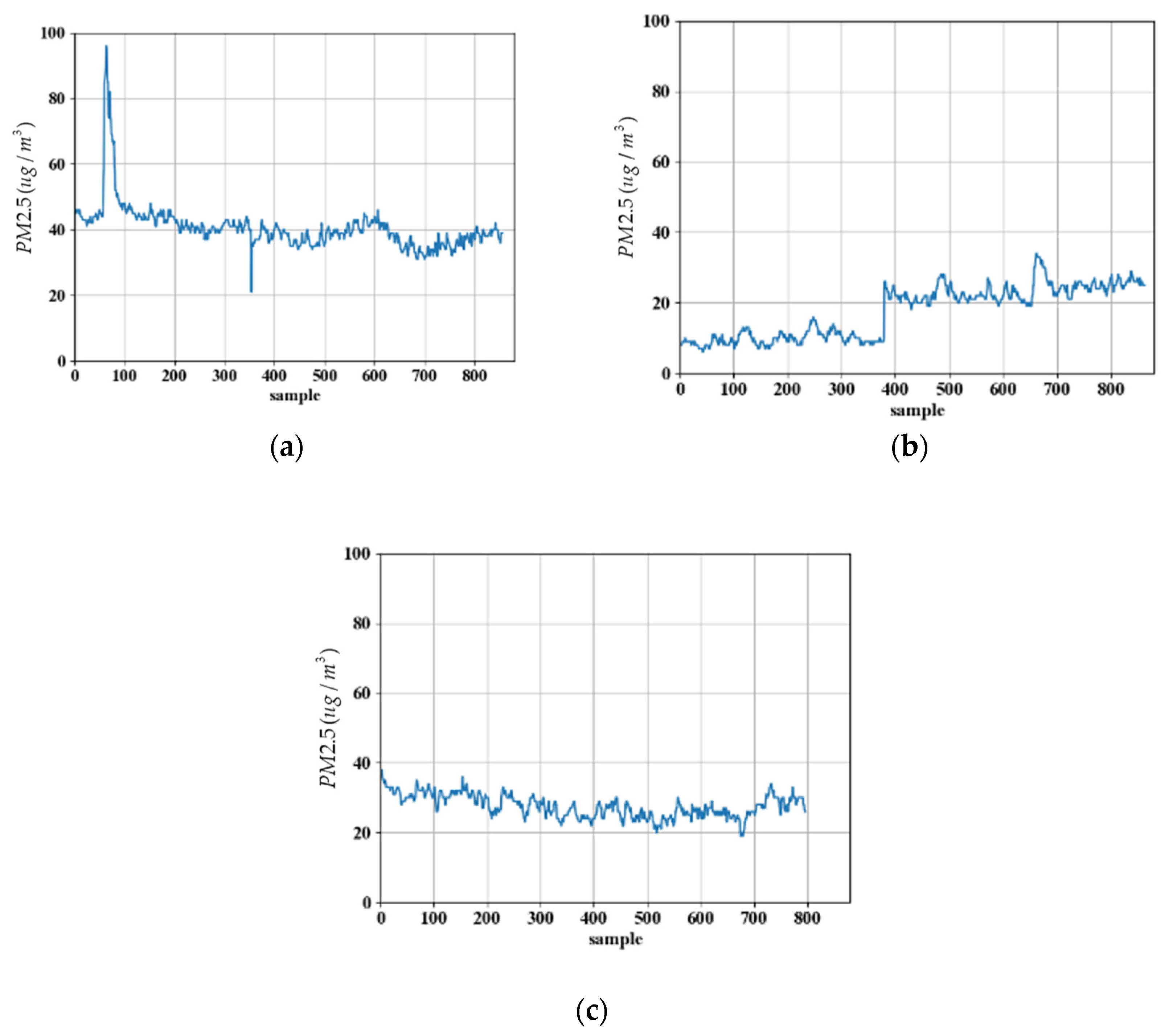
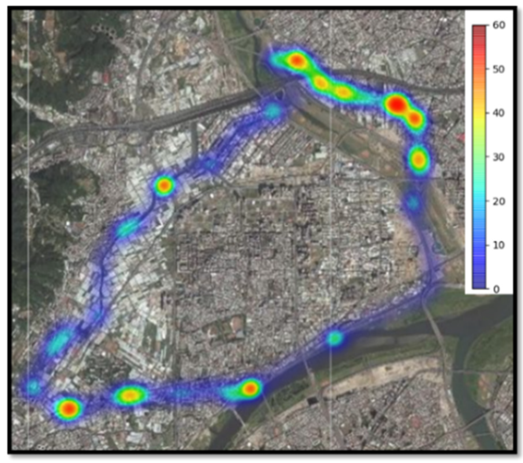
5.1. Measurement Data

Figure 17a–c shows the measured pollution curves at 07:30 P.M. on 15 February 2019; 02:00 and 06:00 P.M. on 28 February 2019; and 04:30 P.M. on 1 March 2019, respectively. Figure 17a displays an abrupt change in the pollutant concentration, in which the PM2.5 value reached 96 μg/m³ for an instant before plunging immediately. This high value was likely caused by a mobile pollution source, such as a dump truck or a vehicle with excessively high exhaust gas emission. Figure 17b depicts data for two periods. A sudden jump in the PM2.5 value is observed at the 379th data point. The left side of the jump represents the data at 02:00 P.M. on 28 February 2019, and the right side of the jump represents the data at 06:00 P.M. on the same day. In Figure 17c, all the PM2.5 values are below 40 μg/m³, and no large fluctuation is observed.

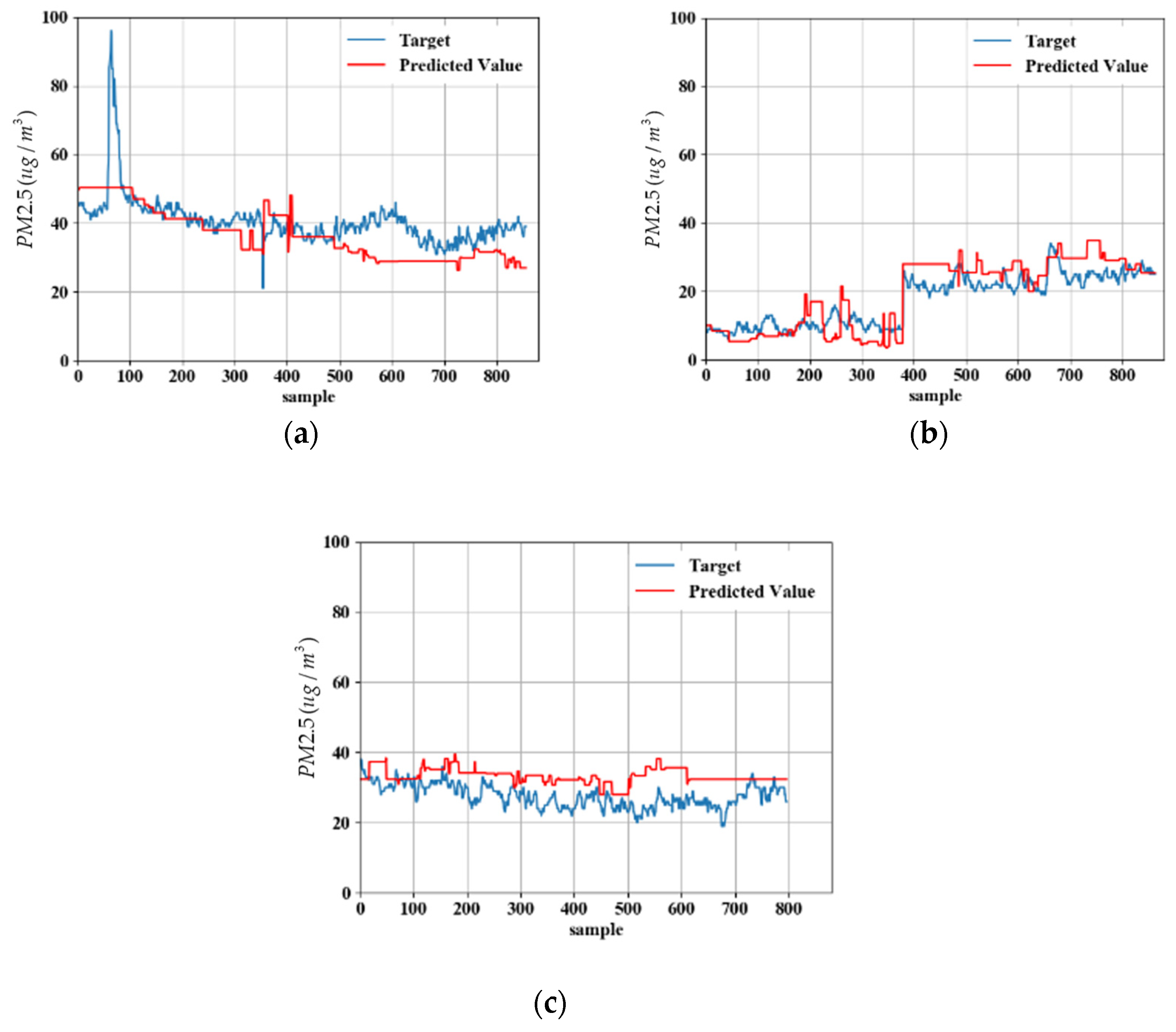
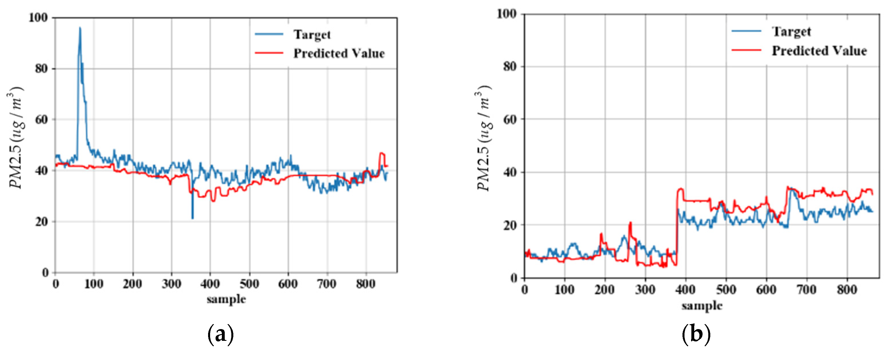
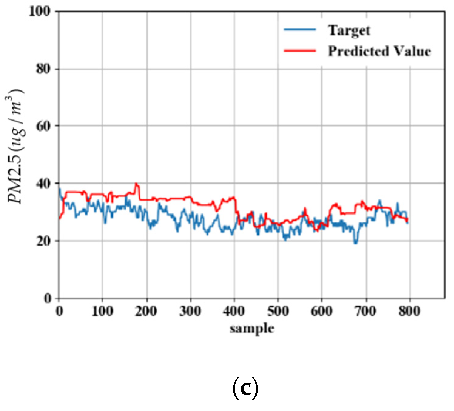
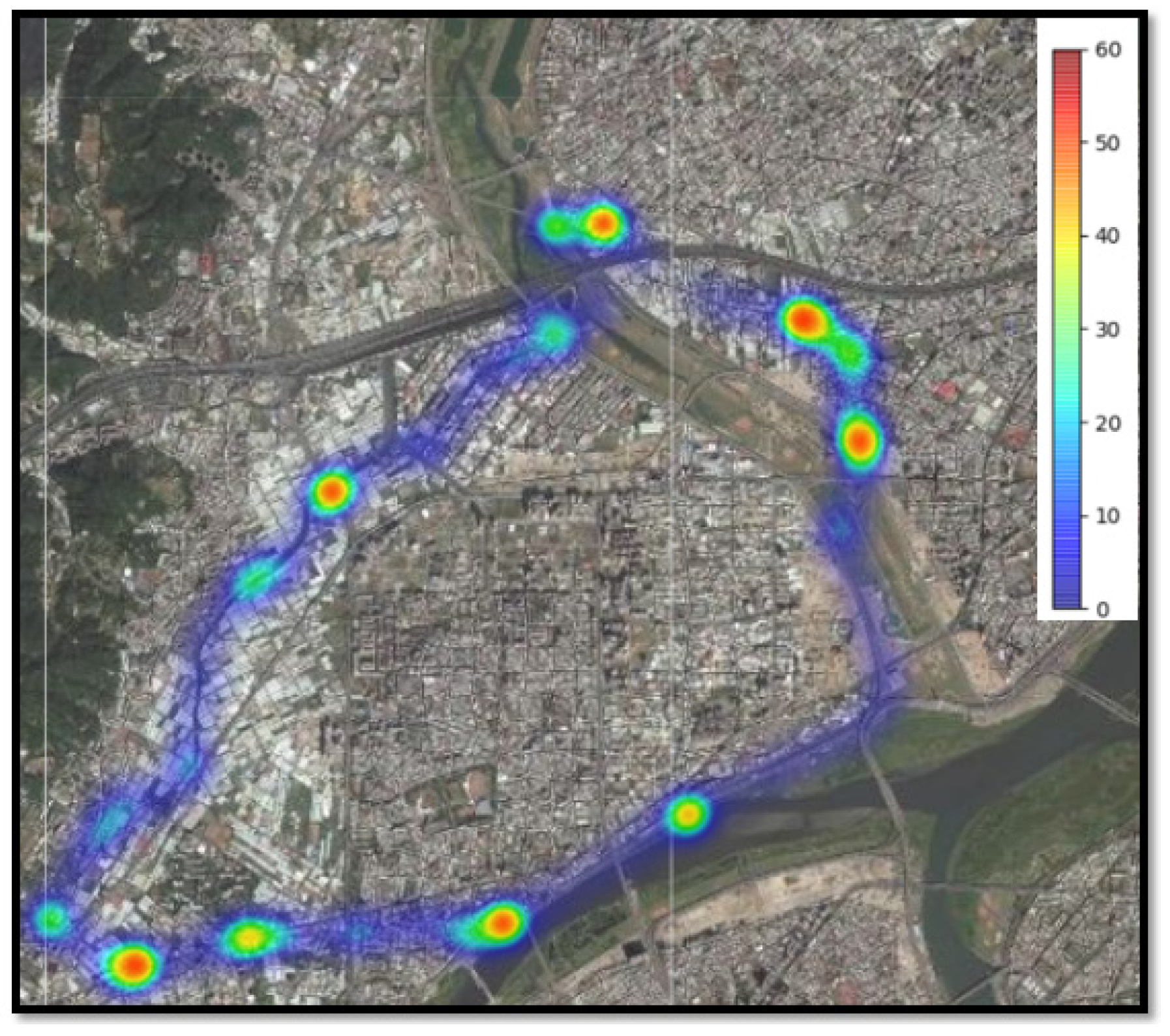
5.2. Model Predicted Data

Figure 18a–c displays the prediction results of the decision tree model. The MAE values based on the results shown in Figure 18a–c are 5.8774, 4.3325, and 5.8248 μg/m³, respectively. The pollution prediction curves of the decision tree model exhibit a stair like shape, which is a result of the features of the decision tree algorithm. The use of a single decision tree may lead to extreme prediction results. For example, in Figure 18a, the predicted values were relatively low compared with the measured values beyond the 500th data point.

Figure 19a–c illustrates the prediction results of the random forest model. The MAE values based on the results shown in Figure 19a–c are 4.6718, 4.5614, and 4.5789 μg/m³, respectively. The random forest model performs random training with a combination of multiple trees to avoid the extreme predictions of a single decision tree. Thus, the predictions of this model had superior generalizability, and the prediction curves did not exhibit a stair like shape. In general, the error of the random forest model’s predictions was approximately 4 μg/m³. Most of the prediction results of this model fell within a reasonable range.

Figure 20a–c displays the prediction results of the multilayer perceptron model. The MAE values based on the results shown in Figure 20a–c were 7.5940, 4.3535, and 8.3501 μg/m³, respectively. For the multilayer perceptron model, only the results in Figure 20b exhibit satisfactory accuracy. The aforementioned model failed to accurately predict the pollution results in the two other periods. Thus, the multilayer perceptron model had substandard generalizability.

Figure 21a–c depicts the prediction results of the RBF neural network model. The MAE values based on the results shown in Figure 21a–c were 7.0793, 3.9603, and 15.1626 μg/m³, respectively. Figure 21c reveals relatively large errors between the prediction results of the RBF neural network model and the measured pollutant concentration values, indicating that this model has marginally insufficient generalizability.

Table 4. MAE values of the learning models.

Estimation Models MAE (μg/m3)
Date	15 February 2019	28 February 2019	1 March 2019
Decision tree	5.8774	4.3326	5.8248
Random forest	4.6718	4.5614	4.5789
Multilayer perceptron	7.5940	4.3535	8.3501
RBF neural network	7.0793	3.9603	15.1626

compares the MAE values of the learning models. The random forest model exhibited stable prediction and the lowest error values overall.

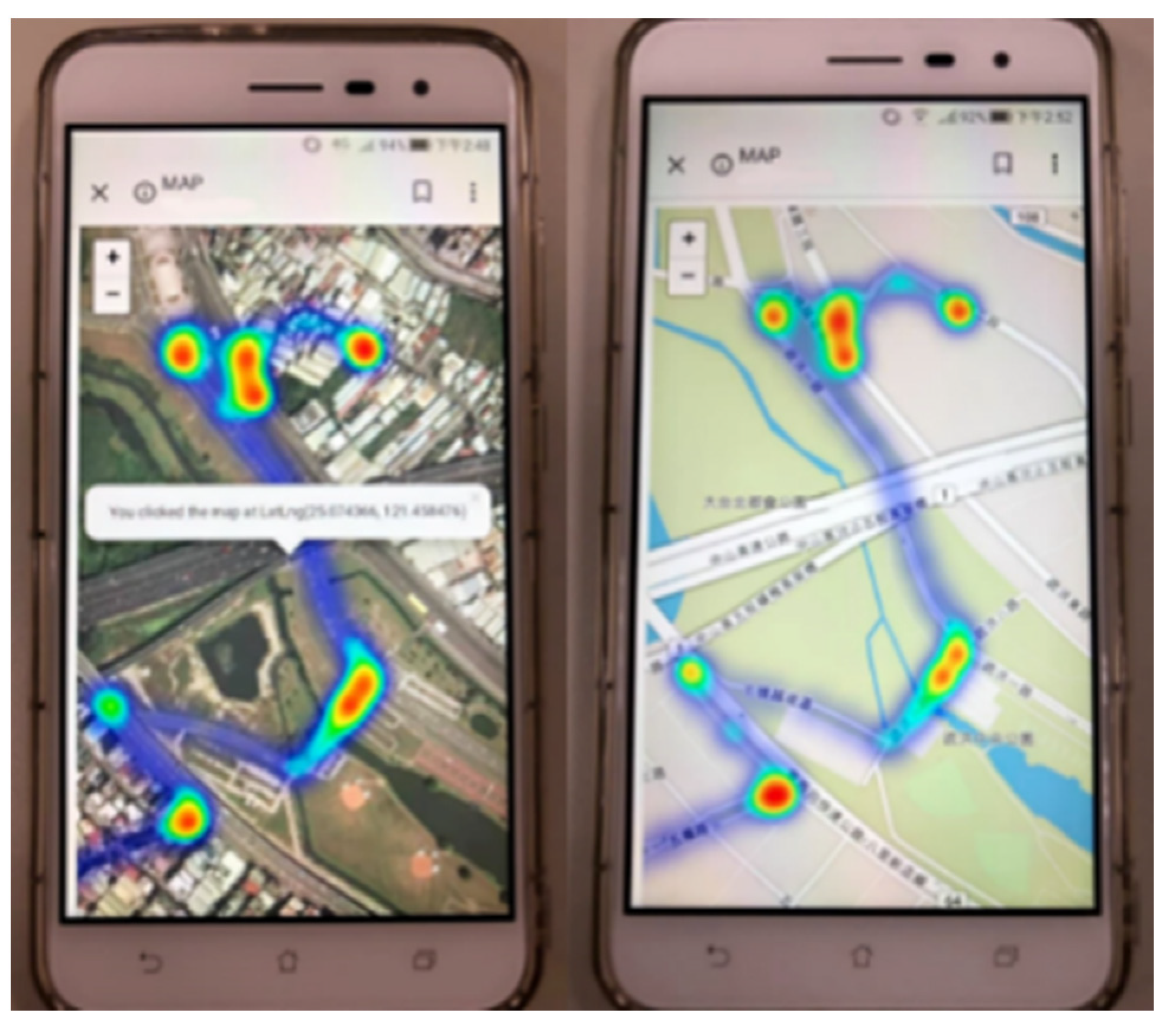
5.3. Web Application

The random forest model provided stable and favorable prediction outcomes. Thus, this model was used as the application model. To visualize the PM2.5 distributions in different regions clearly, a web application was designed in this study. The use of webpages allows users to grasp pollution changes in different areas easily. The web application was constructed using Leaflet, and a heat scale is used to indicate the pollution level. The heat range is set between 0 and 60 μg/m³, and values above 60 μg/m³ are denoted in dark red. Users can zoom in every area of the maps to obtain detailed information.

In this study, the aforementioned application was used to create pollution level maps for two periods, namely 07:30 P.M. on 15 February 2019, and 11:00 P.M. on 14 February 2019. The experiments were conducted with a motorcycle carrying the PM2.5 device and riding around the main roads of New Taipei City to collect data for training and testing. Figure 22 displays the measured pollutant concentrations at 07:30 P.M. on 15 February 2019, and Figure 23 shows the corresponding prediction results. According to the aforementioned figures, the prediction results are mostly consistent with the measurement results. The red squares in the two figures are the intersection on Zhongzheng Road and neighboring roads in Xinzhuang District, both of which are among the most critical traffic sections in Xinzhuang District. A possible reason why these road sections exhibited high pollution levels is that 07:30 P.M. is the rush hour.

Figure 24 shows the measured pollutant concentrations at 11:00 P.M. on 14 February 2019, and Figure 25 illustrates the corresponding prediction results. The measurement results are similar to the prediction results, and most of the areas exhibit low pollution. Luzhou District exhibited marginally higher pollution than the other Districts did. A shortcoming is observed in that the system failed to predict the pollution distribution in the middle section of the Luzhou District.

6. Conclusions

In this study, a PM2.5 pollution prediction system was designed for three urban areas in Taiwan. There are five stages in our designed system: the sensing, data transmission, database, pollution data visualization, and ML stages. According to the experimental results, the real time pollution can be predicted accurately. The systematic information collected can also be shared to government agencies for improvement measures. We can also use these data to remind the public to evacuate mid-city areas or avoid peak hours. Providing the quantitative data to the Health Department as a reference, which may help to prevent respiratory diseases and improve residents’ standards of living.

References

1. Fazziki, A.; Benslimane, D.; Sadiq, A.; Ouarzazi, J.; Sadgal, M. An Agent Based Traffic Regulation System for The Roadside Air Quality Control. IEEE Access 2017, 5, 13192–13201. [Google Scholar] [CrossRef]
2. Hu, K.; Rahman, A.; Bhrugubanda, H.; Sivaraman, V. Hazeest: Machine Learning Based Metropolitan Air Pollution Estimation from Fixed and Mobile Sensors. IEEE Sens. J. 2017, 17, 3517–3525. [Google Scholar] [CrossRef]
3. Kadri, A.; Yaacoub, E.; Mushtaha, M.; Abu-Dayya, A. Wireless Sensor Network for Real time Air Pollution Monitoring. In Proceedings of the IEEE International Conference on Communications, Signal Processing and Their Applications, Sharjah, United Arab Emirates, 12–14 February 2013; pp. 1–5. [Google Scholar]
4. Mead, M.; Popoola, O.; Stewart, G.; Landshoff, P.; Calleja, M.; Hayes, M.; Baldovi, J.; McLeod, M.; Hodgson, T.; Dicks, J.; et al. The Use of Electrochemical Sensors for Monitoring Urban Air Quality in Low-cost, High density Networks. Atmos. Environ. 2013, 70, 186–203. [Google Scholar] [CrossRef] [Green Version]
5. Predić, B.; Yan, Z.; Eberle, J.; Stojanovic, D.; Aberer, K. Exposuresense: Integrating Daily Activities with Air Quality Using Mobile Participatory Sensing. In Proceedings of the IEEE International Conference on Pervasive Computing Communications Workshops, San Diego, CA, USA, 18–22 March 2013; pp. 303–305. [Google Scholar]
6. Shaban, K.; Kadri, A.; Rezk, E. Urban Air Pollution Monitoring System with Forecasting Models. IEEE Sens. J. 2016, 16, 2598–2606. [Google Scholar] [CrossRef]
7. Hasenfratz, D.; Saukh, O.; Walser, C.; Hueglin, C.; Fierz, M.; Thiele, L. Pushing The Spatio temporal Resolution Limit of Urban Air Pollution Maps. In Proceedings of the IEEE International Conference on Pervasive Computing and Communications, Budapest, Hungary, 24–28 March 2014; pp. 69–77. [Google Scholar]
8. Bacco, M.; Delmastro, F.; Ferro, E.; Gotta, A. Environmental Monitoring for Smart Cities. IEEE Sens. J. 2017, 17, 7767–7774. [Google Scholar] [CrossRef]
9. Chen, L.J.; Ho, Y.H.; Hsieh, H.H.; Huang, S.T.; Lee, H.C.; Mahajan, S. ADF: An Anomaly Detection Framework for Large scale PM2.5 Sensing Systems. IEEE Internet Things J. 2018, 52, 559–570. [Google Scholar] [CrossRef]
10. Singh, V.; Carnevale, C.; Finzi, G.; Pisoni, E.; Volta, M. A Cokriging Based Approach to Reconstruct Air Pollution Maps Processing Measurement Station Concentrations and Deterministic Model Simulations. Environ. Model. Softw. 2011, 26, 778–786. [Google Scholar] [CrossRef]
11. Sivaraman, V.; Carrapetta, J.; Hu, K.; Luxan, B.G. HazeWatch: A Participatory Sensor System for Monitoring Air Pollution in Sydney. In Proceedings of the IEEE Conference on Local Computer Networks Workshops, Sydney, Australia, 21–24 October 2013; pp. 56–64. [Google Scholar]
12. Qu, H.; Chan, W.I.; Xu, A.; Chug, K.L.; Lau, K.H.; Guo, P. Visual Analysis of the Air Pollution Problem in Hong Kong. IEEE Trans. Vis. Comput. Graph. 2007, 13, 1408–1415. [Google Scholar] [CrossRef] [PubMed] [Green Version]
13. Gu, K.; Qiao, J.; Lin, W. Recurrent Air Quality Predictor Based on Meteorology and Pollution Related Factors. IEEE Trans. Ind. Inform. 2018, 14, 3946–3955. [Google Scholar] [CrossRef]
14. Boubrima, A.; Bechkit, W.; Rivano, H. Optimal WSN Deployment Models for Air Pollution Monitoring. IEEE Trans. Wirel. Commun. 2017, 16, 2723–2735. [Google Scholar] [CrossRef] [Green Version]
15. Al-Ali, R.A.; Zualkernan, I.; Aloul, F. A Mobile GPRS Sensors Array for Air Pollution Monitoring. IEEE Sens. J. 2010, 10, 1666–1671. [Google Scholar] [CrossRef]
16. Xiaojun, C.; Xianpeng, L.; Peng, X. IoT Based Air Pollution Monitoring and Forecasting System. In Proceedings of the International Conference on Computer and Computational Sciences, Las Vegas, NV, USA, 7–9 December 2015; pp. 257–260. [Google Scholar]
17. Dam, N.; Ricketts, A.; Catlett, B.; Henriques, J. Wearable Sensors for Analyzing Personal Exposure to Air Pollution. In Proceedings of the System and Information Engineering Design Symposium, Charlottesville, VA, USA, 28 April 2017; pp. 1–4. [Google Scholar]
18. Qin, D.; Yu, J.; Zou, G.; Yong, R.; Zhao, Q. A Novel Combined Prediction Scheme Based on CNN and LSTM for Urban PM2.5 Concentration. IEEE Access 2019, 7, 20050–20059. [Google Scholar] [CrossRef]
19. Duangsuwan, S.; Takarn, A.; Nujankaew, R.; Jamjareegulgarn, P. A Study of Air Pollution Smart Sensors LPWAN via NB-IoT for Thailand Smart Cities 4.0. In Proceedings of the IEEE International Conference on Knowledge and Smart Technology, Chiangmai, Thailand, 31 January–3 February 2018. [Google Scholar]
20. Florence, G.; Jason, S.; Martin, W. A machine learning approach to investigating the effects of mathematics dispositions on mathematical literacy. Int. J. Res. Method Educ. 2017, 41, 306–327. [Google Scholar]
21. AFath, H.; Madanifar, F.; Abbasi, M. Implementation of multilayer perceptron (MLP) and radial basis function (RBF) neural networks to predict solution gasoil ratio of crude oil systems. Petroleum 2020, 6, 80–91. [Google Scholar]
Figure 1. System architecture.
Environments 08 00099 g001
Figure 2. Hardware equipment.
Environments 08 00099 g002
Figure 3. Waterproof double layer case.
Environments 08 00099 g003
Figure 4. The process of environment sensing.
Environments 08 00099 g004
Figure 5. Heat distribution in Leaflet.
Environments 08 00099 g005
Figure 6. Location of air quality measurement stations in the Taipei.
Environments 08 00099 g006
Figure 7. Mobile sensing data at 11:00 A.M. on 20 January 2019.
Environments 08 00099 g007
Figure 8. Mobile sensing data at 10:00 A.M. on 3 January 2019.
Environments 08 00099 g008
Figure 9. Structure of the PM prediction model.
Environments 08 00099 g009
Figure 10. Model training process.
Environments 08 00099 g010
Figure 11. Random forest.
Environments 08 00099 g011
Figure 12. Learning results of the decision tree model: (a) training set and (b) testing set.
Environments 08 00099 g012
Figure 13. Learning results of the random forest model: (a) training set and (b) testing set.
Environments 08 00099 g013
Figure 14. Learning results of the multilayer perceptron model: (a) training set and (b) testing set.
Environments 08 00099 g014
Figure 15. Learning results of the RBF neural network model: (a) training set and (b) testing set.
Environments 08 00099 g015
Figure 16. Comparison of the model output results: output results of the (a) decision tree model, (b) random forest model, (c) multilayer perceptron model, and (d) RBF neural network model.
Environments 08 00099 g016
Figure 17. Measured pollutant concentration data: measured values at (a) 07:30 P.M. on 15 February 2019; (b) 02:00 and 06:00 P.M. on 28 February 2019; and (c) 04:30 P.M. on 1 March 2019.
Environments 08 00099 g017
Figure 18. Prediction results of the decision tree model: model prediction results for (a) 15 February, (b) 28 February, and (c) 1 March 2019.
Environments 08 00099 g018
Figure 19. Prediction results of the random forest model: model prediction results for (a) 15 February, (b) 28 February, and (c) 1 March 2019.
Environments 08 00099 g019aEnvironments 08 00099 g019b
Figure 20. Prediction results of the multilayer perceptron model: model prediction results for (a) 15 February, (b) 28 February, and (c) 1 March 2019.
Environments 08 00099 g020
Figure 21. Prediction results of the RBF neural network model: model prediction results for (a) 15 February, (b) 28 February, and (c) 1 March 2019.
Environments 08 00099 g021
Figure 22. Measured pollutant concentrations at 07:30 P.M. on 15 February 2019.
Environments 08 00099 g022
Figure 23. Prediction results for 07:30 P.M. on 15 February 2019.
Environments 08 00099 g023
Figure 24. Measured pollutant concentrations at 11:00 P.M. on 14 February 2019.
Environments 08 00099 g024
Figure 25. Prediction results for 11:00 P.M. on 14 February 2019.
Environments 08 00099 g025