Economic and Life Cycle Analysis of Passive and Active Monitoring of Ozone for Forest Protection

Abstract

At forest sites, phytotoxic tropospheric ozone (O₃) can be monitored with continuously operating, active monitors (AM) or passive, cumulative samplers (PM). For the first time, we present evidence that the sustainability of active monitoring is better than that of passive sensors, as the environmental, economic, and social costs are usually lower in the former than in the latter. By using data collected in the field, environmental, social, and economic costs were analyzed. The study considered monitoring sites at three distances from a control station in Italy (30, 400, and 750 km), two forest types (deciduous and Mediterranean evergreen), and three time windows (5, 10, and 20 years of monitoring). AM resulted in more convenience than PM, even after 5 years, in terms of O₃ depletion, global warming, and photochemical O₃ creation potential, suggesting that passive monitoring of ozone is not environmentally sustainable, especially for long time periods. AM led to savings ranging from a minimum of EUR 9650 in 5 years up to EUR 94,796 in 20 years in evergreen forests. The resulting social cost of PM was always higher than that of AM. The present evaluation will help in the decision process for the set-up of long-term forest monitoring sites dedicated to the protection of forests from O₃.

1. Introduction

Sustainability is a holistic approach that considers ecological, social, and economic dimensions, recognizing that all must be considered together [1]. Sustainability is usually defined as the processes and actions through which humankind avoids the depletion of natural resources in order to keep an ecological balance that does not allow the quality of life of modern societies to decrease. Indeed, the evaluation of the sustainability of different goods or services takes into account environmental, economic, and social impacts [2,3]. Environmental impact assessment includes the emissions into the environment related with the extraction of the raw materials, manufacturing of the products, and resource consumption [3,4]. The manufacturing, use, and disposal of a product involve a series of inputs, in terms of energy and resources, which generates several outputs, in terms of materials and emissions. These contribute to a wide range of impacts on ecosystems and human health, such as climate change, stratospheric ozone (O₃) depletion, tropospheric O₃ formation, eutrophication, acidification, toxicological stress on human health and ecosystems, depletion of resources, water use, land use, and noise [4,5,6,7]. Life cycle assessment (LCA) is the internationally recognized methodology to evaluate the convenience of a good or a service in terms of environmental sustainability (8). Thanks to this methodology, it is possible to assess the entire life cycle of a product, process, or activity to identify, quantify, and environmentally analyze all the inputs and outputs involved in the production, use, and disposal of that product, process, or activity [8,9,10,11].

Forest monitoring is a crucial key step in the protection of forests from different stressors related to air pollution and climate change [12,13,14,15]. Among the air pollutants, tropospheric O₃ is of primary interest for vegetation due to its elevated phytotoxicity, even at ambient concentrations [16]. Indeed, O₃ is recognized as a major concern for plant health, as it impacts crop yield [17], forest growth [18,19], and biodiversity [20]. Ozone is a secondary air pollutant formed in the atmosphere under sunlight from the oxidation of the primary pollutants, nitrogen oxides and volatile organic compounds [21]. Ozone is still a global problem for forest productivity, as highlighted by the analysis of present and future global scenarios [22,23]. The exposure index for forest protection against negative impacts of background O₃ currently used in Europe is the concentration-based index AOT40, defined as the accumulated O₃ dose above 40 ppb during daylight hours over the growing season, although a new index has been proposed as more appropriate, i.e., POD1, defined as the phytotoxic O₃ dose exceeding 1 nmol m⁻² s⁻¹ of stomatal uptake, cumulated over daylight hours during the growing season [24,25]. Both indexes require hourly data to be calculated.

At forest sites, tropospheric O₃ can be monitored with either continuously operating, mechanical, real-time active monitors or passive, cumulative, total exposure samplers [26,27]. The passive system has been used since 2000 in Europe, e.g., at the Level II forest sites of the ICP Forests network [28], while the active system is used at some ICP Forests sites [29]. Passive samplers are characterized by uncertainties that reduce their reliability [30,31], and low temporal resolution, from one week to one month, while POD1 and AOT40 require hourly data. This implies the need to apply functions to estimate hourly concentrations, starting from weekly or biweekly data. Among different methods [31,32,33,34], the ICP Forests manual recommends the use of the Loibl function [35,36,37] to estimate hourly values. There are contrasting results, however, about the actual adequacy of this function in nonhomogeneous territories [38]. The uncertainties in estimating POD1 by passive sampling are discussed in [39], which tested the suitability of using aggregated data instead of hourly data for PODY (POD with variable stomatal uptake threshold (Y)) calculations [39].

An assessment of the environmental impacts of the active and passive systems has never been carried out, but can help evaluating the suitability of the two monitoring methodologies. It is even important to consider the economic consequences of these alternative systems, i.e., determine the cost-effectiveness of the alternative investments [40]. Financial limitations, especially in ecological programs, require a clear identification of costs [41], and the active technique is considered more expensive; active monitors are expensive and require electricity and a safe climate-controlled shelter for effective operation, while passive samplers are inexpensive, easy to use, and require no electricity [42]. At remote sites, the availability of power supply is often limited, and this has been a major limitation to the use of the active O₃ monitoring so far. Nowadays, however, solar panels have relatively low cost and their use, supported by batteries, is a widely adopted solution in remote meteorological stations. In addition, less trips to the forests are required for data collection thanks to remote connection via GPRS for the active monitoring system than for the passive approach. Hence, a comparison of the explicit costs in a defined period is needed to evaluate the cost-effectiveness of the two systems.

To complete the evaluation of the monitoring system sustainability, we calculated the social costs considered here as the social cost of carbon (SCC), which is among the most important pillars in the economics of climate change [43]. SCC is the global cost caused by an additional ton of carbon dioxide (CO₂) emissions or its equivalent [44]; for this reason, it is often combined with LCA studies [45,46]. Indeed, estimates of SCC are used to evaluate climate change policies and cost-benefit analysis of GHG emission reduction projects [43,47].

The aim of the present study is to evaluate, for the first time, the sustainability of active and passive O₃ monitoring at forest plots, analyzing the data in terms of environmental, economic, and social costs. We hypothesized that (1) the expected higher costs of active monitoring are compensated over time, and, thus, we performed our analyses over different time windows (i.e., 5, 10, and 20 years of monitoring); (2) differences depend on the seasonal duration of the monitoring, and, thus, we compared two sites dominated by either deciduous (April-to-September growing season) or Mediterranean evergreen (year-long) trees; (3) the distance between monitoring sites and the control station could be relevant in terms of costs, and, thus, we compared sites at 30, 400, and 750 km from the control station.

2. Materials and Methods

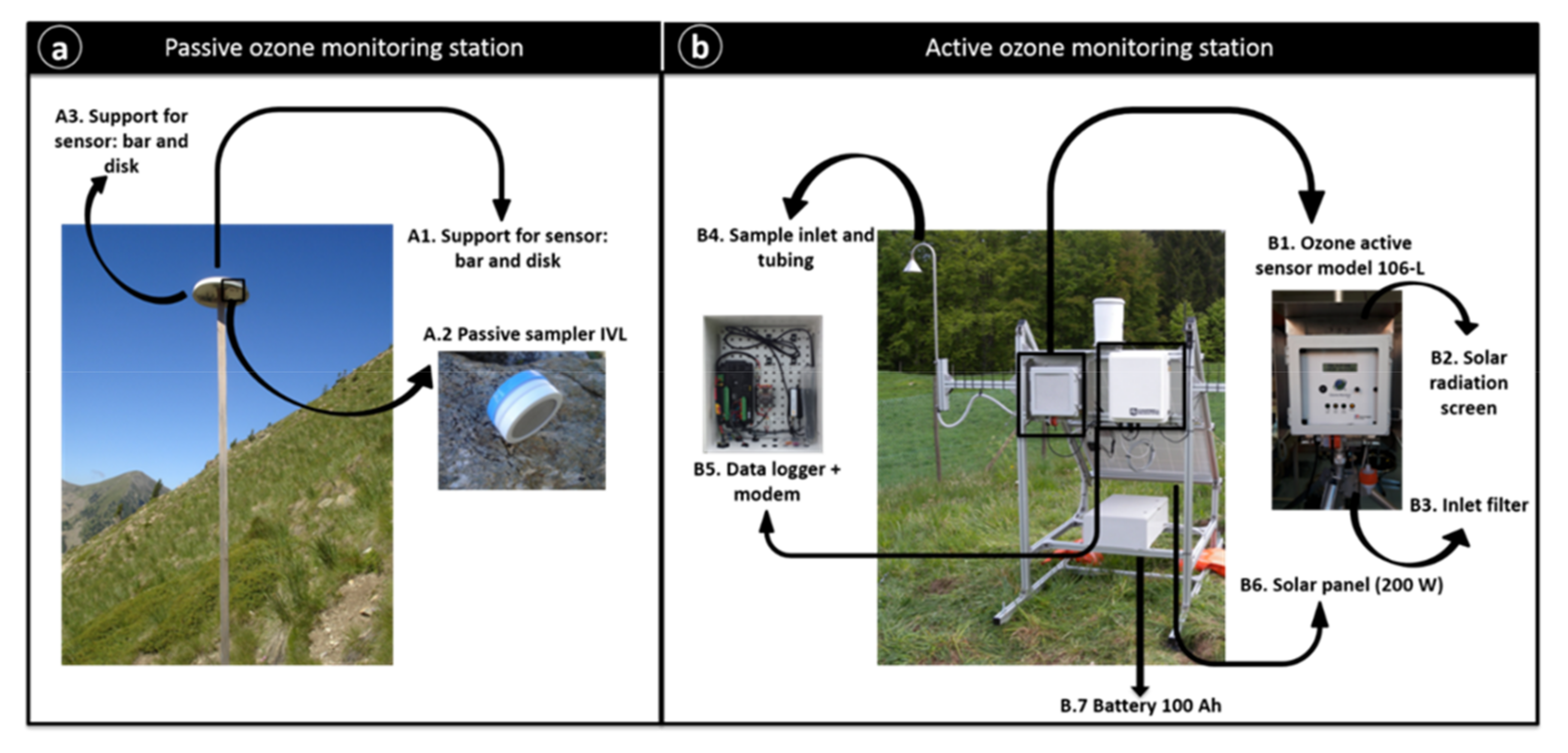
2.1. Description of the Two Monitoring Methods

ICP Forests establishes a specific protocol for passive O₃ monitoring (PM), but it does not recommend a specific category of samplers. Hence, this study followed the ICP Forests manual [13] and applied the protocol to the two most common passive sampler types used by scientists, i.e., Institutet for Vatten-och Luftvadsforskning (IVL) [48] and Ogawa & Co., Inc., Gifu, Japan and types [49,50].

The passive samplers are filters without any system of air control. Both Ogawa and IVL samplers must be installed at forest sites at a height of about two meters above ground, supported by a steel bar planted into the ground (Figure 1a A1). At least two replicates (Figure 1a A2) must be simultaneously exposed at each site and located in protective shelters (Figure 1a A3) in order to reduce eventual environmental disturbances. According to the European protocol [13], the sampling is carried out on a 2-week basis and covers the period 1 April–30 September. For Mediterranean conditions (evergreen species), it is recommended to monitor the whole year (1 January–31 December). In the present analysis, data collection in the evergreen Mediterranean forest was conducted every month in the six months from October to March (when O₃ concentrations are expected to be lower), and every two weeks in the growing season from April to September (

Table 1. Number of trips and work time (WT) for each trip from the central station to the forest site for two case studies at a similar distance from the station, i.e., evergreen Mediterranean (EF) and deciduous (DF) forests, and three time windows, i.e., 5, 10, and 20 years of monitoring. Simulations are based on the data collected during the 5-year project MOTTLES [29].

	Passive Monitoring IVL/OGAWA						Active Monitoring
Items	5 Years		10 Years		20 Years		5 Years		10 Years		20 Years
	N. Trips	WT (h)	N. Trips	WT (h)	N. Trips	WT (h)	N. Trips	WT (h)	N. Trips	WT (h)	N. Trips	WT (h)
Deciduous forest
Installation	1	14.25	1	14.25	1	14.25	1	28.5	1	28.5	1	28.5
Maintenance activity	0	0	0	0	1	14.25	20	28.5	40	28.5	80	28.5
Extraordinary maintenance	/		/		/		1	28.5	2	28.5	5	28.5
Data collection	60	14.25	120	14.25	240	14.25	/		/		/
Evergreen forest
Installation	1	14.25	1	14.25	1	14.25	1	28.5	1	28.5	1	28.5
Maintenance activity	0	0	0	0	1	14.25	20	28.5	40	28.5	80	28.5
Extraordinary maintenance	/		/		/		1	28.5	2	28.5	5	28.5
Data collection	90	14.25	180	14.25	360	14.25	/		/		/

). Transport and storage of the passive samplers before and after exposure may have an influence on the chemical analysis; thus, the protocol described in the ICP Forests manual [13] must be strictly followed. For quality control, at least four blank samplers per season should be included in the standard transport and storage procedures. After sampler collection, filters are immersed into extraction solutions placed in clean plastic vials. The vials are then stored in a refrigerator at 4 °C until analysis made by ion chromatography. To prepare the filters for analysis, the following equipment and supplies are needed: calibrated automatic dispensing pipette (5 mL); forceps, not serrated, sharp with curved tip; IC vials (0.5 mL for Dionex auto-sampler); caps for IC vials; syringes, 3 mL disposable; Millex-LCR13 syringe filters [51].

In the active monitoring (AM), O₃ is measured by means of an active sensor. We used the Model 106 L (2B Technologies, Inc., Boulder, CO, USA; Figure 1b B1), which is a common active O₃ monitor in forest AM [51]. Ozone monitors must be protected by solar radiation with a specific screen (Figure 1b B2). Data are recorded by a data logger (Campbell scientific in our case, Figure 1b B5). The data acquisition interval is 10 s and the average is stored every hour. Thanks to a GPR connection, data are transmitted to a file transfer protocol (FTP) server via a GPRS modem (Figure 1b B5). In AM, air is sampled through the sample inlet (Figure 1b B4), passing through a particle filter (Figure 1b B3) that needs to be replaced every 3 months. A monitor calibration is required once per year. In addition, battery replacement is required every 4 years. Power supply is assured by solar panels (Figure 1b B6) or mains, when present, and backup batteries to be used in case of power failure (Figure 1b B7).

2.2. Analyzed Factors

To test our hypotheses, the environmental, monetary, and social analyses of the two PM and AM systems were implemented by 2 case studies (deciduous forest—DF and evergreen Mediterranean forest—EF with O₃ monitoring over the growing seasons, i.e., April to September and all year round, respectively) and 3 time windows (5, 10, and 20 years of monitoring duration). The time windows were selected as low (5 years), medium (10 years), and long-term (20 years) on the basis of the supposed average life of the solar panel needed for power supply in the AM. To have comparable results, the DF and EF case sites were selected at a fixed distance from the control station (a research center in Italy). The distance of the two forest sites from the control station was 335 km for VEN1 (DF site in Pian del Cansiglio (Belluno), dominated by Fagus sylvatica) and 355 km for CPZ1 (EF site in Castel Porziano (Rome), dominated by Quercus ilex). The distance is representative because the average distance of all the 17 monitoring sites of the MOTTLES network [29] from the control station was 400 km. Therefore, 400 km was considered as an average distance between research center and forest plot, with a maximum and minimum distance of 700 and 30 km, respectively. All data on materials, personnel, and travels used for LCA, economic, and social analysis corresponded to real data collected for VEN1 and CPZ1. Within AM, the cost in DF did not differ from the cost in EF (and, thus, only one value was shown).

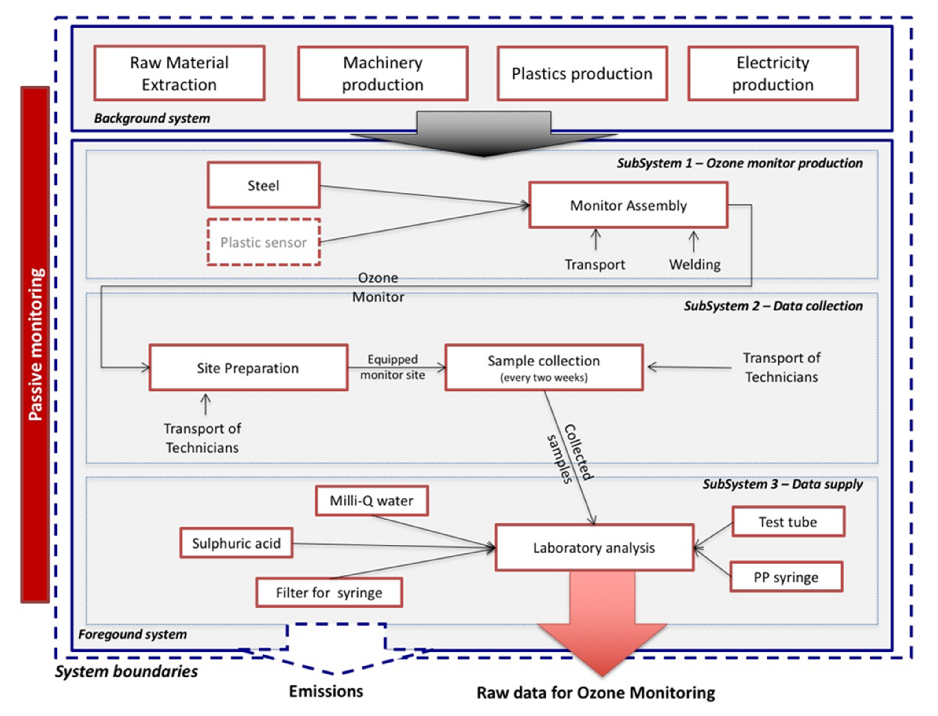
2.2.1. Definition of System Boundaries and Functional Unit

A system of pollutant monitoring is normally built to provide information, generally related with a series of values referred to a specific time frame (e.g., average concentration per day, maximum and minimum per hour, etc.). AM does not need laboratory analysis, while PM does. Materials, energy, and emissions related to the activities carried out to finalize O₃ monitoring, in both AM and PM, were included in the LCA analysis. In particular, the system boundaries for both the analyzed monitoring systems included production, installation, and maintenance of monitoring stations (including sensors, energy suppliers, fence, etc.), energy and materials used during monitoring periods, and maintenance and data collection activities. Travel of technicians from the research center to the plot site was also considered. In PM, despite the simpler composition of the remote station, many travels are required to collect the filters in the field. Travel needs are reduced with AM, given that data collection is done by remote. The described information was classified as primary data, being obtained by interviews to producers of monitoring systems and to researchers and technicians who work in O₃ monitoring. The background information, such as raw material extraction, machinery, and plastics production, and electricity production and supply, were collected by internationally recognized databases. The use of information provided by the system monitoring can be very different depending on the activities carried out by research centers, public health laboratories, etc. For this reason, the analysis made in this study stops when the information on O₃ concentration is available for the final user. Moreover, the disposal of the monitoring stations was not considered due to the lack of real experience in this field. Finally, in this study, a cradle-to-gate analysis was carried out.

All the identified inputs and outputs have to be referred to a functional unit, which allows the comparison between the two systems. In this study, the functional unit was defined as: “the biweekly supply of atmospheric O₃ concentrations (ppb) over one year”. It is important to underline that the chosen functional unit is based on the capacity of the passive sampler to supply information every two weeks. The AM gives more frequent and detailed information than the PM, but the comparison between the two systems is suitable because they are considered as alternatives by scientists [26,29,52,53].

2.2.2. Definition of Subsystems

To implement the inventory (LCI—Life Cycle Inventory) (International Organization for Standardization, 2006) and to clearly identify the inputs and outputs in the main phases of life cycle, three subsystems were identified and defined in the two flow charts and system boundaries (Figure 2 and Figure 3): (i) the production of O₃ monitors (AM) or samplers (PM); (ii) the on-site preparation, installation, operation, and maintenance of the monitoring system; and (iii) data collection and (only for PM) laboratory analysis.

• → Subsystem 1—Ozone monitor production

In this subsystem, the main processes involved in O₃ monitor production were identified, and reliable data of materials and energy consumptions related with their production were collected, mainly by interviews to producers and analysis of the products. The main raw materials for monitors were aluminum and steel. Active systems were more complex than passive ones, with a higher weight and more structures and devices (such as solar panels, battery). In passive systems, the plastic sensor was not considered (Figure 1a A2) due to the difficulties in understanding the type of material used and the production process. This missing information was considered as negligible due to the minimum weight and related inputs and emissions. In active systems, the production processes and materials used in the analysis were assimilated to the most suitable components/materials available on databases.

• → Subsystem 2—Preparation, installation, operation, and on-site maintenance of the monitoring systems

In this subsystem, the devices considered in subsystem 1 were the input, and were added to the materials needed to install the remote monitoring station. Active systems require electricity to work; for this reason, a photovoltaic panel with all the additional components needed to guarantee energy supply to the active monitor (inverter, battery, cables, supports, etc.) were considered. These inputs were not applied in the passive system, which does not require energy in the field. In this subsystem, the travels (by car) of technicians and researchers needed to collect samples (passive system) and to make maintenance interventions were also considered (Table 1). The type of forest influenced the number of travels in PM, as the number of samples to be collected in one year varied and was higher in EF, while it did not affect AM because the number of travels for maintenance was not related with the length of the data collection period.

• → Subsystem 3—Data supply

In this subsystem, all the processes, from information collected in the field to the raw data available for stakeholders, were included. This subsystem was important mainly for passive systems, because it included laboratory analysis of passive samplers. Data about laboratory activities were obtained thanks to the available protocols and interviews with technicians. Active samplers sent to the research center, calculation of the O₃ concentration data, and inputs related to the data transfer system were included in Subsystem 2.

For each subsystem, primary data were collected by interviews to producers of monitoring systems and to researchers and technicians who work in O₃ monitoring. The background information, such as raw material extraction, machinery and plastics production, and electricity production and supply, were collected by internationally recognized databases (GaBI, Ecoinvent). An overall summary of the LCI, including background processes from databases, was reported for both PM (

Table 2. Summarized inventory of inputs and outputs referred to the case study of ozone monitoring with passive sensors. The initial acronyms in “applied processes” refer to geographic location: “RER” = Europe; “GLO” = global; “Row” = rest of the world.

	Input		Amount	Unit	Applied Processes
Travel (installation and maintenance)	Travels by car		800	km	RER: transport, passenger car, small size, petrol, EURO 5, <u-so>. Ecoinvent 3.3
	Gasoline		40.3	kg	RoW: market for petrol, low-sulfur. Ecoinvent 3.3
	Road allocation		0.6	Ecoinvent quantity (ma)	RoW: market for road. Ecoinvent 3.3
	Tire consumption		−0.059	kg	GLO: market for tire wear emissions. Ecoinvent 3.3
	Road consumption		−0.010	kg	GLO: market for road wear emissions. Ecoinvent 3.3
	Brake consumption		−0.005	kg	GLO: market for brake wear emissions. Ecoinvent 3.3
	Ordinary maintenance of car		0.005	n	GLO: market for passenger car maintenance. Ecoinvent 3.3
Passive sensors	Structure		10	kg	RoW: sheet rolling, chromium steel. Ecoinvent 3.3
	Welding		2	m	RoW:welding arc, steel. Ecoinvent 3.3
Laboratory analysis	Test tube	Production	0.01	kg	RoW: extrusion production, plastic pipes <u-so>. Ecoinvent 3.3
		Electricity	2.36 × 10−4	MJ	GLO: market group for electricity, high voltage. Ecoinvent 3.3
		Heat	0.00683	MJ	Europe without Switzerland: market for heat, district or industrial, other than natural gas. Ecoinvent 3.3
		Lubricants	1.43 × 10−6	kg	GLO: market for lubricating oil. Ecoinvent 3.3
		Waste recycling	3.68 × 10−5	kg	Europe without Switzerland: market for waste plastic, mixture. Ecoinvent 3.3
		PP granulate	4.98 × 10−6	kg	GLO: market for polypropylene, granulate. Ecoinvent 3.3
	Syringe	Syringe production	0.0025	kg	RoW: extrusion production, plastic pipes <u-so>. Ecoinvent 3.3
		Electricity	1.64 × 10−5	MJ	GLO: market group for electricity, high voltage. Ecoinvent 3.3
		Heat	0.00171	MJ	Europe without Switzerland: market for heat, district or industrial, other than natural gas. Ecoinvent 3.3
		Lubricants	3.58 × 10−7	kg	GLO: market for lubricating oil. Ecoinvent 3.3
		Waste recycling	9.23 × 10−6	kg	Europe without Switzerland: market for waste plastic, mixture. Ecoinvent 3.3
		PP granulate	1.25 × 10−6	kg	GLO: market for polypropylene, granulate. Ecoinvent 3.3
	Filter for syringe	Filter for syringe production	0.0005	kg	RoW: extrusion production, plastic film <u-so>. Ecoinvent 3.3
		Electricity	1.53 × 10−5	MJ	GLO: market group for electricity, high voltage. Ecoinvent 3.3
		Heat	0.00011	MJ	Europe without Switzerland: market for heat, district or industrial, other than natural gas. Ecoinvent 3.3
		Lubricants	5.25 × 10−8	kg	GLO: market for lubricating oil. Ecoinvent 3.3
		Waste recycling	1.21 × 10−5	kg	Europe without Switzerland: market for waste plastic, mixture. Ecoinvent 3.3
		PP granulate	2.44 × 10−8	kg	GLO: market for polyvinylidenchloride, granulate. Ecoinvent 3.3
	Milli-Q water		22.58	kg	GLO: market for water, ultrapure. Ecoinvent 3.3
	Sulfuric acid		0.0513	kg	GLO: market for sulfuric acid. Ecoinvent 3.3

) and AM (

Table 3. Summarized inventory of inputs and outputs referred to the case study of ozone monitoring with active sensors. The initial acronyms in “applied processes” refer to geographic location: “RER” = Europe; “GLO” = global; “Row” = rest of the world.

		Input	Amount	Unit	Applied Processes
Travel (installation and maintenance)		Travels by car	800	km	RoW: transport, passenger car, small size, petrol, EURO 5, <u-so>. Ecoinvent 3.3
		Gasoline	40.3	kg	RoW: market for petrol, low-sulfur. Ecoinvent 3.3
		Road allocation	0.6	Ecoinvent quantity (ma)	RoW: market for road. Ecoinvent 3.3
		Tire consumption	−0.059	kg	GLO: market for tire wear emissions. Ecoinvent 3.3
		Road consumption	−0.010	kg	GLO: market for road wear emissions. Ecoinvent 3.3
		Brake consumption	−0.005	kg	GLO: market for brake wear emissions. Ecoinvent 3.3
		Ordinary maintenance of car	0.005	n	GLO: market for passenger car maintenance. Ecoinvent 3.3
Active monitor	Steel	Steel extrusion	0.31	kg	RoW: impact extrusion of steel, cold, 1 stroke <u-so>. Ecoinvent 3.3
		Compressed air	0.09	m3	GLO: market for compressed air, 700 kPa gauge. Ecoinvent 3.3
		Finite element modeling	0.31	kg	GLO: market for impact extrusion of steel, cold, 1 stroke. Ecoinvent 3.3
		Modeling machine	1.22 × 10−5	kg	RoW: metal working machine production, unspecified. Ecoinvent 3.3
		Allocation working factory	1.42 × 10−10	Unit	GLO: market for metal working factory. Ecoinvent 3.3
		Preparatory steel treatments	0.31	kg	GLO: market for impact extrusion of steel, cold, tempering. Ecoinvent 3.3
			0.31	kg	GLO: market for impact extrusion of steel, cold, initial surface treatment. Ecoinvent 3.3
	Aluminum	Aluminum extrusion	0.81	kg	RoW: impact extrusion of aluminium, 1 stroke <u-so>. Ecoinvent 3.3
		Compressed air	0.235	m3	GLO: market for compressed air, 700 kPa gauge. Ecoinvent 3.3
		Finite element modeling	0.81	kg	GLO: market for impact extrusion of aluminum, deformation stroke. Ecoinvent 3.3
		Modeling machine	3.20 × 10−5	kg	RoW: metal working machine production, unspecified. Ecoinvent 3.3
		Allocation working factory	3.71 × 10−10	Unità di lavoro	GLO: market for metal working factory. Ecoinvent 3.3
		Aluminum extrusion	0.81	kg	RoW: impact extrusion of aluminum, 1 stroke <u-so>. Ecoinvent 3.3
		Preparatory aluminum treatments	0.81	kg	GLO: market for impact extrusion of aluminum, cold, tempering. Ecoinvent 3.3
			0.81	kg	GLO: market for impact extrusion of aluminum, cold, initial surface treatment. Ecoinvent 3.3

).

2.2.3. Life Cycle Impact Assessment (LCIA)

Data collected in LCI were implemented by software (GaBi version 7.3), and the environmental assessment LCIA was conducted by characterization factors included in CML 2001 (update January 2016). Six impact categories were analyzed: acidification potential (AP), eutrophication potential (EP), global warming potential (GWP), human toxicity potential (HTP), ozone layer depletion potential (ODP), photochemical ozone creation potential (POCP). The results of LCIA were organized in two main categories of emissions: (i) “travel” to the monitoring site and back for sample collection (PM) and maintenance (both PM and AM), and (ii) “material”, which included all the components of monitors (PM and AM) and the materials used in laboratory analysis.

2.3. Environmental Costs

The guidelines established by ISO 14,040 (International Organization for Standardization, 2006) were applied to compare the environmental profile of the two methods for forest O₃ monitoring through life cycle assessment (LCA). The implementation of a comparative LCA for two or more services requires the definition of comparable systems and a suitable functional unit, which will be the term of comparison. In this study, the analysis was applied to a service (O₃ monitoring) that supplies a set of information (values of O₃ concentration) for a defined period. Following ISO standards, all the required phases were implemented, including life cycle inventory (LCI) and life cycle impact assessment (LCIA) (International Organization for Standardization, 2006). The two systems were analyzed by considering the same input and output categories, and excluding eventual information available for only one of the two systems.

2.4. Economic Costs

In order to compare the costs of AM, PM-Ogawa, and PM-IVL, we defined the following three cost categories:

- Materials. We considered the monitor devices and the complementary material (structures, power supply tools, etc.) in the case of AM and PM.

- Personnel. The total working days were quantified on the basis of MOTTLES activities. The unitary cost was calculated as the hourly rate of a technician effectively employed in the MOTTLES project for the year 2017 (taxes included according to Italian regulation).

- Travels. For installation, data collection, and maintenance, field visits by operators are required (as explained above). Considering the average 400 km of distance between the remote and the central sites, we calculated the total km travelled by car, and related costs.

Table 4. Costs of active monitoring station items listed separately per installation, ordinary maintenance, extraordinary maintenance, and data collection for deciduous forests (DF) and evergreen Mediterranean forests (EF). fr., frequency.

Item	Cost (€)	n. per Site	fr. (Times/Year)
INSTALLATION
Materials/consumables
Ozone Monitor model 106-L 2bTECH	4456	1	0
Ozone Monitor enclosure	426	1	0
Ozone sensor screen	101.5	1	0
Solar screen	102	1	0
Inlet filter	4	1	0
Data acquisition system
Data logger Campbell CR 300	2100	1	0
Protective box	350	1	0
Modem	300	1	0
Support structure + power supply system with photovoltaic panels +assembly material	3197	1	0
Sample inlet and tubing	359.3	1	0
Battery (100 Ah)	80	1	0
Personnel (hourly rate)	31.5	28.5	0
Travels	68.4	2	0
EXTRAORDINARY MAINTAINANCE
Materials/consumables
Replacement parts (pump, lamp, battery)	1046.15	1	0.2
Personnel	31.5	28.5	0.2
Travels	68.4	2	0.2
ORDINARY MAINTAINANCE
Scrubber	58.7	1	1
Filter	4	1	6
Personnel	31.5	28.5	4
Travels	68.4	2	4
DATA COLLECTION
Cost for data transmission via GPRS (SIM card)	50	1	1

,

Table 5. Costs of passive monitoring station items with OGAWA sensors, listed separately per installation, ordinary maintenance, and data collection for deciduous forests (DF) and evergreen Mediterranean forests (EF). Extraordinary maintenance is not required.

Item	Cost (€)	n. per Site	fr.
INSTALLATION
Materials/consumables
Passive sampler OGAWA with airtight storage vial (including components) + pad	109.6	2	0
Support for sensor: steel bar	4	1	0
Personnel	31.5	14.25	0
Travels	68.4	2	0
ORDINARY MAINTAINANCE
Personnel per DF	31.5	1	12 t/y
Personnel per EF	31.5	1	18 t/y
Travels per DF	68.4	2	12 t/y
Travels per EF	68.4	2	18 t/y
121 travels (12/y)	820.8
DATA COLLECTION
Analyses and filters per DF	40.2	2	12 t/y
Analyses and filters per EF	40.2	2	18 t/y

and

Table 6. Total cost of passive monitoring station items with IVL sensors, listed separately per installation, ordinary maintenance, and data collection for deciduous forests (DF) and evergreen Mediterranean forests (EF). Extraordinary maintenance is not required.

Item	Cost (€)	n. per Site	fr.
INSTALLATION
Materials/consumables
Passive sampler IVL with airtight storage vial (including components) + pad	55	2	0
Support for sensor: steel bar	4	1	0
Personnel	31.5	14.25	0
Travels	68.4	2	0
ORDINARY MAINTAINANCE
Personnel per DF	31.5	1	12 t/y
Personnel per EF	31.5	1	18 t/y
Travels per DF	68.4	2	12 t/y
Travels per EF	68.4	2	18 t/y
121 travels (12/y)	820.8
DATA COLLECTION
Analyses and filters per DF	55	2	12 t/y
Analyses and filters per EF	55	2	18 t/y

list the components to calculate the amount of each cost category (materials, personnel, and travels) for AM, PM-OGAWA, and PM-IVL divided into installation, ordinary maintenance/data collection, and extraordinary maintenance. For AM, costs for each item were considered as the cost effectively incurred for the installation, maintenance, and data collection of the MOTTLES sites in 2017.

To simulate the three time scenarios, we calculated the monetary present value, PV₀, at the first year of installation (2017) of all the installations and future maintenance costs, assuming an installation duration, T, of 5, 10, or 20 years. The present value formula is as follows:

$$P{V}_0={\displaystyle \sum }_{t=1}^T\frac{C_t}{{\left(1+r\right)}^t}$$

(1)

where C_t is the annual cost at the year t (5, 10, or 20 years from installation), and r is a 5% discount rate [54]. National governments assume discount rates ranging between 3.5% and 15%, and 5% is considered a value coherent with average market interest rates and discounts adopted to calculate the social cost of carbon [55].

2.5. Social Costs

As for the monetary cost, we compared the present value of the social costs of annual CO₂ emissions caused by the management of the two monitoring systems. Emissions accumulation in the atmosphere would cause loss of productivity in many economic sectors and health-related impacts. These outcomes can be translated into monetary terms, and thus adopted to evaluate the costs and benefits of emission reduction control. The SCC reflects the present value of such future costs caused by an additional ton of CO₂. Therefore, it represents the monetary value of the future global damages done by emitting one more ton of carbon today [56]. The literature supplies a strand of SCC values, depending on climate change projection damage modeling [57]. We used the values developed by the US EPA (Interagency Working Group on Social Cost of Greenhouse Gases, 2016), since they are officially utilized by the US Federal Government for cost-benefit analysis [58], while equivalent guidelines at EU levels are not yet available. EPA provides SCC at different social discount rates; in fact, sensitivity analysis is fundamental to provide a range of future options in a context of uncertainty about the future damages of climate change. Thus, we calculated the total SCC over 5, 10, and 20 years of AM and PM by using SC-CO₂ values provided by EPA at a social discount rate of 5%. These values are reported in EUR 2019.

3. Results

3.1. Environmental Assessment

The environmental profiles of PM and AM were different depending on the time window considered as the monitoring duration (

Table 7. Results of LCIA for a monitoring site at a distance of 400 km. PM, Passive monitoring; AM, active monitoring; DF, deciduous forest; EF, evergreen Mediterranean forest. Impact categories: AP= Acidification Potential; EP= Eutrophication Potential; GWP= Global Warming Potential; HTP= Human Toxicity Potential; ODP= Ozone layer Depletion Potential; POCP= Petrochemical Ozone Creation Potential. For each time scenario (5, 10 and 20 years from installation), total emissions are reported in different colours that highlight the best (green), worst (red) and intermediate (orange).

		5 years			10 years			20 years
		PM-DF	PM-EF	AM	PM-DF	PM-EF	AM	PM-DF	PM-EF	AM
AP [kg SO2-Equiv.]	Travel	25.1	37.5	9.1	49.8	74.5	17.7	99.2	148.6	35.0
	Material	0.8	1.1	45.7	1.5	2.2	69.0	2.9	4.3	115.5
	Total	25.9	38.6	54.8	51.3	76.7	86.7	102.1	152.9	150.5
EP [kg Phosphate-Equiv.]	Travel	6.9	10.3	2.5	13.7	20.5	4.9	27.3	40.8	9.6
	Material	0.5	0.7	7.0	0.9	1.4	8.9	1.9	2.8	12.6
	Total	7.4	11.0	9.5	14.6	21.9	13.8	29.1	43.6	22.3
GWP 100 years [kg CO2-Equiv.]	Travel	10,886	16,240	3926	21,594	32,302	7674	43,009	64,425	15,169
	Material	131	193	1094	255	379	1344	503	751	1844
	Total	11,018	16,433	5020	21,849	32,681	9018	43,513	65,176	17,013
HTP inf. [kg DCB-Equiv.]	Travel	3163	4718	1141	6273	9384	2229	12,495	18,716	4407
	Material	108	140	4322	171	234	5960	298	424	9235
	Total	3271	4858	5463	6445	9619	8189	12,792	19,140	13,642
ODP [kg R11-Equiv.]	Travel	1.91E-03	2.85E-03	6.89E-04	3.79E-03	5.67E-03	1.35E-03	7.55E-03	1.13E-02	2.66E-03
	Material	2.04E-05	3.04E-05	1.20E-04	4.04E-05	6.03E-05	1.43E-04	8.03E-05	1.20E-04	1.90E-04
	Total	1.93E-03	2.88E-03	8.09E-04	3.83E-03	5.73E-03	1.49E-03	7.63E-03	1.14E-02	2.85E-03
POCP [kg Ethene-Equiv.]	Travel	5.3	8.0	1.9	10.6	15.9	3.8	21.1	31.7	7.5
	Material	0.1	0.1	2.1	0.1	0.2	3.1	0.3	0.4	5.1
	Total	5.4	8.1	4.0	10.7	16.1	6.9	21.4	32.1	12.6

). In the case of Mediterranean evergreen forests (year-long), AM was better than PM, except for acidification (AP) and human toxicity potential (HTP) over 5 years and AP over 10 years. In the case of deciduous forests (April–September growing season), PM had better results than PM in EF, being the best monitoring strategy in terms of AP and HTP in all time frames, as well as eutrophication potential (EP) over 5 years. In short, AM was generally a better option than PM in terms of emissions for longer monitoring periods, i.e., 10–20 years and year-long growing season, except for AP and HTP. The main reason behind these results is related to travels. Indeed, PM requires frequent accesses to the site, which means a high number of travels to and from the site. AM requires more instruments and materials but less resources in terms of human presence. For these reasons, the environmental profiles are influenced mainly by travels for PM and by materials for AM, and this is the reason why AM is better in the longer periods while PM is better in the shorter periods. Moreover, travels are the environmental hotspot for PM in all the impact categories, being the cause of more than 90% of total emissions in all the cases. For this reason, in some impact categories heavily influenced by the emissions of car engines, such as global warming potential (GWP), the environmental profile of AM was always better than that of PM, with high differences in terms of total emissions. A detailed analysis of each impact category is found below.

3.1.1. Acidification Potential (AP)

Total emission of sulfuric acid equivalents was higher for AM than for PM in most of the examined cases, and PM-DF was always better than PM-EF. In fact, AM was better than PM only in the 20-year scenario when compared with PM-EF. In all cases, PM-DF was better than AM, especially in the 5- and 10-year scenarios. The shorter the period of monitoring, the higher the differences between AM and PM. In the 5-year monitoring, AM was 111% higher than PM-DF and 42% higher than PM-EF, while the difference decreased over 10 and 20 years; in this last case, the value of SO₂eq for AM was 47% higher than PM-DF, and about 1% lower than PM-EF. Materials and travels had different importance in determining the emissions of the two types of monitoring; travels were the cause of more than 97% of total SO₂eq emissions in all cases, while, in AM, materials were the environmental hotspot for AP, being at least 76.8% of total emissions (up to 83.5% in 5-year monitoring).

3.1.2. Eutrophication Potential (EP)

The emission of Peq was the highest in PM-EF. In the passive systems, EP was mainly related to travels (always over 93% of total emissions), while, in the AM, travels never influenced more than 44% of the total emissions. In terms of total emissions, PM-DF were the best for 5-years monitoring, while AM was the best for 10 and 20 years. In fact, emissions of phosphate equivalents were 29% higher for AM than PM-DF in 5 years, while PM-DF was 6% and 31% higher than AM after 10 and 20 years of monitoring, respectively.

3.1.3. Global Warming Potential (GWP)

This impact category was measured as the total amount of CO₂eq. In all examined cases, AM showed markedly lower emissions than PM, in both DF and EF. In the 5-year monitoring, PM in DF showed double emission than that of AM, and PM-EF CO₂eq emitted was three times the CO₂eq emitted in AM. The difference in emissions increased over longer monitoring; in fact, after 20 years, PM in deciduous forest and in evergreen forests was 156% and 283% higher than AM, respectively. Travels had a key role in GWP, contributing up to 98.8% of CO₂eq emissions in PM, and from 78.2% (5 years) to 89.2% (20 years) in AM.

3.1.4. Human Toxicity Potential (HTP)

HTP was expressed as 1,4-dichlorobenzene equivalents/kg emission (DCBeq). As for AP, in DF, PM showed the best environmental profile in comparison with AM, which was 67%, 27%, and 7% higher after 5, 10, and 20 years of monitoring, respectively. Regarding EF, PM was better (11% lower emissions of DCBeq) than AM in the 5-year time window, while it is the worst in 10 and 20 years of monitoring duration (17.5% and 40% higher). While travels related with data collection were the environmental hotspot in PM, in AM, the highest contribution to HTP was related to the materials used in the monitoring station (79% to 68% of total emissions from the 5-year to 20-year time window).

3.1.5. Ozone Layer Depletion Potential (ODP)

For this impact category, the potential impact was reported as trichlorofluoromethane equivalent emissions (kg CFC-11eq), with higher emissions for PM than for AM. Overall, CFC emissions were low, with the highest values occurring in the case of PM in every time window and both forest types, and the highest amount of emissions concentrated on travels (from 85% in AM to 98% in PM).

3.1.6. Photochemical Ozone Creation Potential (POCP)

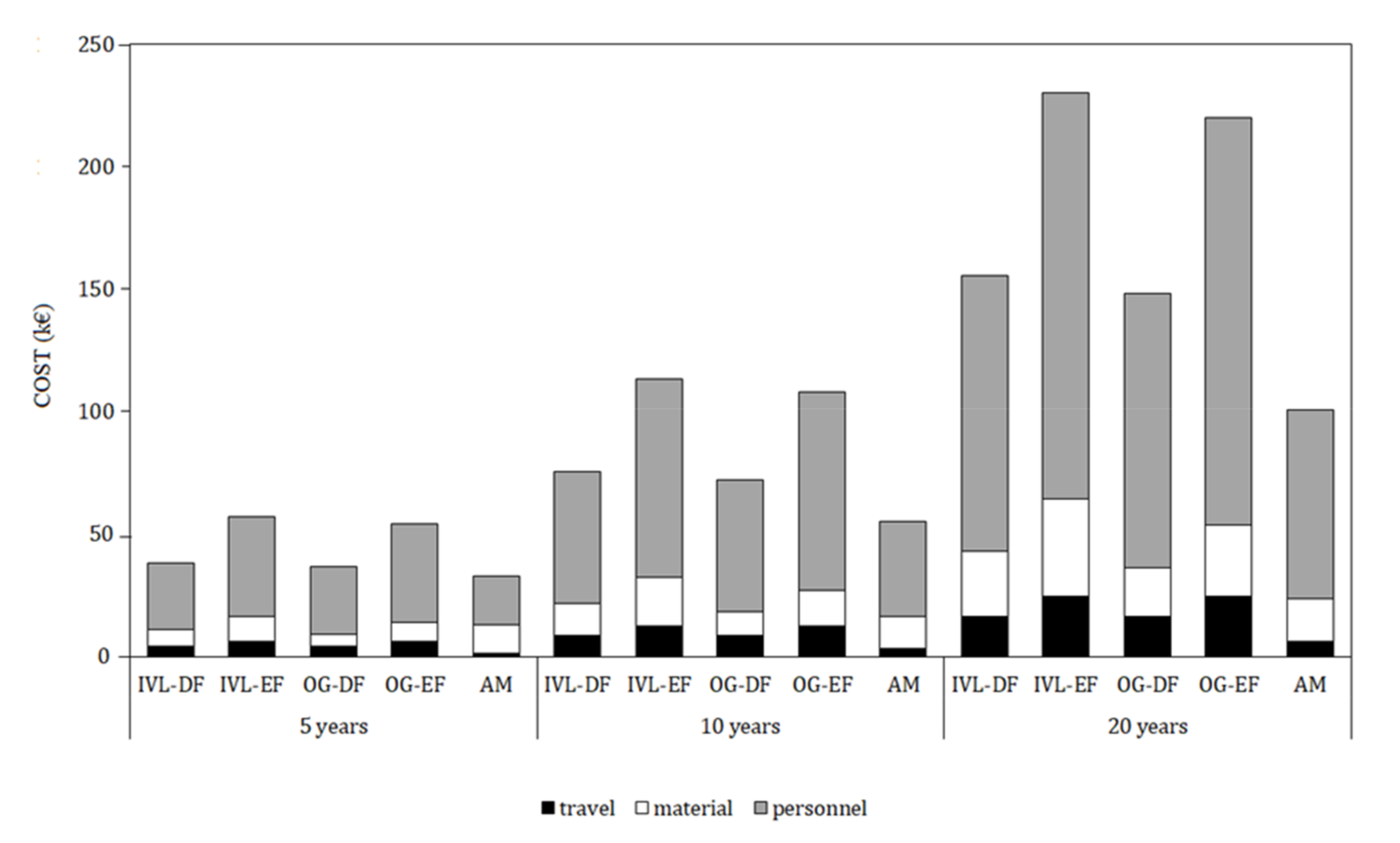
This category evaluated the emission of ethene equivalent (C₂H₄eq) as reference for potential photochemical oxidant creation. The emissions were lower in AM than in PM for both forest types. The total impact of AM was from 34% (5-years) to 70% lower (20-years) than PM in DF. In EF, the difference was higher and emissions of C₂H₄eq in PM were 100%, 133%, and 155% higher than in AM for 5-, 10-, and 20-year monitoring, respectively.

3.2. Economic Costs

No marked differences were observed between Ogawa and IVL passive sensors (Figure 4). AM resulted in the most convenient system, as the costs at 5 years from installation were 33% and 37% lower than PM in DF and 56% and 58% lower than PM in EF. At 10 and 20 years, the monetary savings of AM were even higher, as the costs of the two passive systems were, on average, 49% and 66% lower than PM in DF and EF at 10 years, and 55% and 70% lower at 20 years for OG and IVL, respectively. The cost category material varied with the type of monitoring, while travel and personnel were constant costs for both OGAWA and IVL passive systems within the same type of forest. The cost category that mainly affected all monitoring costs was personnel, representing between 60.2% and 75.6% of the total cost. The personnel had the lowest cost in AM (EUR 7749, EUR 13,820, and EUR 22,305 in 5, 10, and 20 years, respectively) and the highest cost in the two PM systems for evergreen forests (EUR 34,870, EUR 62,192, and EUR 100,372 in 5, 10, and 20 years, respectively). The amount of personnel cost was followed by material (13.5–35.3%) and travels (4.5–11.5%). The lowest cost for the material was calculated for OG-DF: EUR 3898, EUR 7561, and EUR 12,135 at 5, 10, and 20 years, respectively. The highest material cost was calculated for AM in each time scenario, with the highest percentage over the shortest 5-year period (35.3%). Regarding the travel category, the highest costs were attributed to both types of PM for evergreen forests: EUR 2665, EUR 4753, and EUR 7671 in the three time windows, respectively.

3.3. Social Costs

The SCC of PM for sites at a distance of 400 km from the control station result was always higher than the SCC of AM (Figure S1) (see Supplementary Materials). Within PM, the SCC related with the monitoring of EF was EUR 253, 480, and 863 after 5, 10, and 20 years, respectively, i.e., ca. 50% higher than in DF, regardless of the time window. The SCC of AM was EUR 78, 134, and 228, i.e., 60, 58, and 54% lower than PM-DF, and 74, 72, and 69% lower than PM-EF after 5, 10, and 20 years, respectively. In total, AM showed markedly lower CO₂ equivalent emissions than PM, both in DF and EF, leading to a saving of EUR 1563 in DF and EUR 2982 in EF after 5 years per the 400-km site. Those savings increased up to EUR 3185 and EUR 5890 in DF and EF after 10 years, and to EUR 5920 and EUR 10,791 in DF and EF after 20 years.

4. Discussion

The debate between passive and active monitoring has been a pressing dilemma in assessing air pollution at remote forest sites [26,27,29,30,31]. For the first time, we present observational evidence that the sustainability of active monitoring is now better than that of passive sensors, as the environmental, economic, and social costs are usually lower in AM than in PM. In detail, we found a greater environmental sustainability of the active system after 10 years from installation, while social and economic impacts of the active system were lower, even after 5 years. The type of forest determined important differences, as the costs of PM for Mediterranean evergreen forests were always higher than those for deciduous forests; hence, in this forest type, the convenience of the active system is realized earlier. These results were seriously affected by the high costs of personnel in Italy, where our case studies were applied. Our approach warrants further studies in different countries across a range of forest and economic conditions.

4.1. Environmental Sustainability

The results of the environmental impact assessment highlighted an important role of personnel transport on the total amount of emissions. This is a common result obtained in similar studies applied to different sectors, when the analyzed system has low emissions; in these cases, secondary processes become important contributors to the total amount of emissions [59], while, in many other cases, the role of personnel transport is negligible in comparison with the overall emissions [60]. As travels were the major environmental hotspot in our analysis, the influence of travel distance was further investigated by two short-range (30 km) and long-range (750 km) scenarios to quantify the role of distance in terms of total emissions. The LCIA was repeated for both scenarios, considering the same LCI as the case study, changing only the travel distance. PM was almost totally influenced by travel distance, from 93% in EP to 99% in ODP, while AM had a strong component of other inputs (materials) that attenuated the effects of travels on total emissions (Figure S2). In fact, in the 30-km scenario PM had a better environmental profile than AM. On the contrary, in the 750-km scenario, AM was often better than PM. In detail, in the short-range scenario, PM (in both EF and DF) had lower emissions than AM in acidification, eutrophication, human toxicity, and O₃ creation potential (POCP) in all time frames, while in ODP AM was always better than PM-EF and better than PM-DF in the 10 and 20 year time frames; regarding total emissions of CO₂eq (GWP), AM was always better than PM-EF, but not PM-DF, in the 5- and 10-year scenarios. On the other hand, in the long-range scenario AM had a better environmental profile than PM for eutrophication, global warming, O₃ layer depletion, and O₃ creation potential in all time windows and forest types; regarding acidification potential, PM was better than AM only in the 5- and 10-year scenarios in deciduous forests.

4.2. Economic Sustainability

When LCA is combined with an economic analysis, results are more policy relevant, as supported by previous studies [40,61,62]. Similar to other studies conducted in forests, e.g., woody product supply [63,64], the cost category that mainly affected costs in the present study was personnel, suggesting possible different results for monitoring comparisons conducted in countries with different labor costs. As PM requires more frequent travels and, thus, also higher costs of personnel, the monetary cost was always lower for AM. Despite the higher installation costs, AM led to savings ranging from a minimum of EUR 9650 in 5 years in the case of DF up to EUR 94,796 in the case of EF after 20 years. In particular, in the short term, the personnel costs for the collection of PM data exceeded the high cost of AM installation, confirming the convenience of AM. The cost of AM material was lower than that of IVL-EF in the medium term, and of IVL-DF and OG-EF in the long term, suggesting the possibility for managers to replace the passive with the active system in both forest types. The economic convenience of the active system was confirmed in both the long- and short-distance scenarios (Figure S3), despite the large difference among those scenarios in terms of travel contribution to the total costs (from a maximum of 1% in the 30-km scenario to a maximum of 19.5% in the 750-km scenario).

About the passive systems, OGAWA was more convenient than IVL in every case. Such results were related to a lower cost of data analysis; hence, results could change if analysis would be conducted within the research center without extra costs.

4.3. Social Sustainability

Very few studies [45,65] calculated the social cost of the CO₂eq. assessed by the LCA analysis, and it is also probable that none of them included a monetary cost analysis. Then, the present study represents a first experience in the assessment of the three pillars of sustainability (environmental, economic, and social) in the ozone monitoring of forests.

SCC confirmed AM as the most convenient monitoring system, also, in terms of social costs in both forest types, even after 5 years, with a higher convenience at 10 and 20 years. This is not surprising, since SCC is directly related with the global warming potential assessed by LCA.

By applying the distance scenario also to the social impacts, we found that the SCC determined by AM was always lower than PM for the 750-km scenario (savings from EUR 3158 up to EUR 20,483), since travels represented the cause of more than 90% of total emission (Figure S1); in contrast, in the 30-km scenario, PM showed an SCC lower than AM for DF in the medium term (10 years), and for DF and EF in the short term (5 years). A further sensitivity analysis, considering different discount rates, was realized in order to estimate the maximum social cost of both methods. In particular, according to US EPA, we also considered the high-impact scenario, which considers lower-probability, higher-impact outcomes of climate change that would be particularly harmful to society and, thus, relevant to the public and policymakers (calculated as the 95th percentile of the frequency distribution of SC-CO₂ estimates based on a 3% discount rate). Under this scenario, after 20 years, the SCC of AM reached EUR 2201, while PM was EUR 5544 in DF and EUR 8301 in EF (Figure S1).

5. Conclusions

This LCA study estimated the three types of cost associated to active or passive ozone monitoring in forest plots. These innovative results support active O₃ monitoring rather than passive monitoring. Indeed, despite the high installation costs that make active monitoring still little used, the costs of active monitoring are already compensated after 5 years of monitoring due to the large incidence of personnel costs on sample collection in passive monitoring. The advantage of active monitoring is greater in the longer monitoring windows, e.g., for the evergreen Mediterranean forests requiring all-year-long monitoring. The advantage of AM compared to PM is driven by the lower number of trips from the research center to forest sites. In particular, the reduced global warming potential of active monitoring leads to social benefits quantified in terms of social cost of carbon. These results indicated an advantage of active monitoring from an environmental, economic, and social point of view. In addition, the active system supplies reliable hourly data that are suitable for stomatal O₃ flux estimation, supporting policymakers in assessing ozone impacts on forests.

References

1. Moore, J.E.; Mascarenhas, A.; Bain, J.; Straus, S.E. Developing a comprehensive definition of sustainability. Implement. Sci. 2017, 12, 110. [Google Scholar] [CrossRef] [PubMed]
2. Daily, G.C.; Polasky, S.; Goldstein, J.; Kareiva, P.M.; Mooney, H.A.; Pejchar, L.; Ricketts, T.H.; Salzman, J.; Shallenberger, R. Ecosystem services in decision making: Time to deliver. Front. Ecol. Environ. 2009, 7, 21–28. [Google Scholar] [CrossRef] [Green Version]
3. Endris, K.; Marco, T.; Sergio, T.; Gokan, M. Integration of sustainability in NPD process: Italian Experiences. In Proceedings of the PLM 2011—The IFIP WG51—8th International Conference on Product Lifecycle Management, Eindhoven, The Netherlands, 11–13 July 2011. [Google Scholar]
4. Rebitzer, G.; Ekvall, T.; Frischknecht, R.; Hunkeler, D.; Norris, G.; Rydberg, T.; Schmidt, W.P.; Suh, S.; Weidema, B.P.; Pennington, D.W. Life cycle assessment: Part 1: Framework, goal and scope definition, inventory analysis, and applications. Environ. Int. 2004, 30, 701–720. [Google Scholar] [CrossRef] [PubMed]
5. Zhang, Y.I.; Singh, S.; Bakshi, B.R. Accounting for Ecosystem Services in Life Cycle Assessment, Part I: A Critical Review. Environ. Sci. Technol. 2010, 44, 2232–2242. [Google Scholar] [CrossRef] [PubMed]
6. Pennington, D.W.; Norris, G.; Hoagland, T.; Bare, J.C. Environmental comparison metrics for life cycle impact assessment and process design. Environ. Prog. 2000, 19, 83–91. [Google Scholar] [CrossRef]
7. Pennington, D.; Potting, J.; Finnveden, G.; Lindeijer, E.; Jolliet, O.; Rydberg, T.; Rebitzer, G. Life cycle assessment Part 2: Current impact assessment practice. Environ. Int. 2004, 30, 721–739. [Google Scholar] [CrossRef]
8. Wenzel, H.; Hauschild, M.; Alting, L. (Eds.) Environmental Assessment of Products; Kluwer Academic Publisher: Dordrecht, The Netherlands, 1997; Volume 1. [Google Scholar]
9. Baumann, H.; Tillman, A.-M. The Hitch Hiker’s Guide to LCA.; The Authors and Student Literature: Lund, Sweden, 2004. [Google Scholar]
10. Klein, D.; Wolf, C.; Schulz, C.; Weber-Blaschke, G. 20 years of life cycle assessment (LCA) in the forestry sector: State of the art and a methodical proposal for the LCA of forest production. Int. J. Life Cycle Assess. 2015, 20, 556–575. [Google Scholar] [CrossRef]
11. Laschi, A.; Marchi, E.; González-García, S. Environmental performance of wood pellets’ production through life cycle analysis. Energy 2016, 103, 469–480. [Google Scholar] [CrossRef]
12. McLaughlin, S.; Percy, K. Forest Health in North America: Some perspectives on Actual and Potential Roles of Climate and Air Pollution. Water Air Soil Pollut. 1999, 116, 151–197. [Google Scholar] [CrossRef]
13. Schaub, M.; Calatayud, V.; Ferretti, M.; Brunialti, G.; Lövblad, G.; Krause, G.; Sanz, M.J. Part XV: Monitoring of Air Quality. In Manual on Methods and Criteria for Harmonized Sampling, Assessment, Monitoring and Analysis of the Effects of Air Pollution on Forests; UNECE ICP Forests Programme Co-ordinating Centre, Ed.; Thünen Institute of Forest Ecosystems: Eberswalde, Germany, 2016. [Google Scholar]
14. Convention on Long-range Transboundary Air Pollution. Mapping Critical Levels for Vegetation, Chapter III of Manual on Methodologies and Criteria for Modelling and Mapping Critical Loads and Levels and Air Pollution Effects, Risks and Trends. Available online: http://icpmapping.org/Publications_CLRTAP (accessed on 16 July 2018).
15. Totsuka, T.; Sase, H.; Shimizu, H. Major activities of acid deposition monitoring network in East Asia (EANET) and related studies. In Plant Responses to Air Pollution and Global Change; Springer: Tokyo, Japan, 2005; pp. 251–259. [Google Scholar] [CrossRef]
16. Braun, S.; Schindler, C.; Rihm, B. Growth losses in Swiss forests caused by ozone: Epidemiological data analysis of stem increment of Fagus sylvatica L. and Picea abies Karst. Environ. Pollut. 2014, 192, 129–138. [Google Scholar] [CrossRef] [PubMed]
17. De Marco, A.; Screpanti, A.; Paoletti, E. Geostatistics as a validation tool for setting ozone standards for durum wheat. Environ. Pollut. 2010, 158, 536–542. [Google Scholar] [CrossRef] [PubMed]
18. Paoletti, E. Impact of ozone on Mediterranean forests: A review. Environ. Pollut. 2006, 144, 463–474. [Google Scholar] [CrossRef]
19. Mills, G.; Sharps, K.; Simpson, D.; Pleijel, H.; Broberg, M.; Uddling, J.; Jaramillo, F.; Davies, W.J.; Dentener, F.; Van den Berg, M.; et al. Ozone pollution will com-promise efforts to increase global wheat production. Glob. Chang. Biol. 2018, 24, 3560–3574. [Google Scholar] [CrossRef] [PubMed]
20. Agathokleous, E.; Feng, Z.; Oksanen, E.; Sicard, P.; Wang, P.; Saitanis, C.J.; Araminiene, V.; Blande, J.D.; Hayes, F.; Calatayud, V.; et al. Ozone affects plant, insect and soil microbial communities: A threat to terrestrial ecosystems and biodiversity. Sci. Adv. (in press). 2020. [Google Scholar] [CrossRef]
21. Krupa, S.V.; Manning, W.J. Atmospheric ozone: Formation and effects on vegetation. Environ. Pollut. 1988, 50, 101–137. [Google Scholar] [CrossRef]
22. Sicard, P.; Augustaitis, A.; Belyazid, S.; Calfapietra, C.; de Marco, A.; Fenn, M.; Bytnerowicz, A.; Grulke, N.; He, S.; Matyssek, R.; et al. Global topics and novel approaches in the study of air pollution, climate change and forest ecosystems. Environ. Pollut. 2016, 213, 977–987. [Google Scholar] [CrossRef]
23. Aw, J.; Kleeman, M.J. Evaluating the first-order effect of intra annual temperature variability on urban air pollution. J. Geophys. Res. Atmos. 2003, 108, D12. [Google Scholar] [CrossRef]
24. Lefohn, A.S.; Malley, C.S.; Smith, L.; Wells, B.; Hazucha, M.; Simon, H.; Naik, V.; Mills, G.; Schultz, M.G.; Paoletti, E.; et al. Tropospheric ozone assessment report: Global ozone metrics for climate change, human health, and crop/ecosystem research. Elem. Sci. Anthol. 2018, 6, 28. [Google Scholar] [CrossRef] [Green Version]
25. Anav, A.; De Marco, A.; Proietti, C.; Alessandri, A.; Cionni, I.; Dell’Aquila, A.; Friedlingstein, P.; Khvorostyanov, D.; Menut, L.; Paoletti, E.; et al. Comparing concentration-based (AOT40) and stomatal uptake (PODY) metrics for ozone risk assessment to European forests. Glob. Chang. Biol. 2016, 22, 1608. [Google Scholar] [CrossRef] [PubMed]
26. Bytnerowicz, A.; Godzik, B.; Frączek, W.; Grodzińska, K.; Krywult, M.; Badea, O.; Barančok, P.; Blum, O.; Černy, M.; Godzik, S.; et al. Distribution of ozone and other air pollutants in forests of the Carpathian Mountains in central Europe. Environ. Pollut. 2001, 116, 3–25. [Google Scholar] [CrossRef]
27. Hůnová, I.; Livorová, H.; Ostatnická, J. Potential ambient ozone impact on ecosystems in the Czech Republic as indicated by exposure index AOT40. Ecol. Indic. 2003, 3, 35–47. [Google Scholar] [CrossRef]
28. Calatayud, V.; Schaub, M. Methods for Measuring Gaseous air Pollutants in Forests. Dev. Environ. Sci. 2013, 12, 375–384. [Google Scholar] [CrossRef]
29. Paoletti, E.; Alivernini, A.; Anav, A.; Badea, O.; Carrari, E.; Chivulescu, S.; Conte, A.; Ciriani, M.; Dalstein-Richier, L.; De Marco, A.; et al. Toward stomatal-flux based forest protection against ozone: The MOTTLES approach. Sci. Total. Environ. 2019, 691, 516–527. [Google Scholar] [CrossRef] [PubMed]
30. Krupa, S.; Legge, A. Passive sampling of ambient, gaseous air pollutants: An assessment from an ecological perspective. Environ. Pollut. 2000, 107, 31–45. [Google Scholar] [CrossRef]
31. Tuovinen, J.-P. Assessing vegetation exposure to ozone: Is it possible to estimate AOT40 by passive sampling? Environ. Pollut. 2002, 119, 203–214. [Google Scholar] [CrossRef]
32. Cox, R.M. The use of passive sampling to monitor forest exposure to O3, NO2 and SO2: A review and some case studies. Environ. Pollut. 2003, 126, 301–311. [Google Scholar] [CrossRef]
33. Krupa, S.; Nosal, M.; Peterson, D.L. Use of passive ambient ozone (O3) samplers in vegetation effects assessment. Environ. Pollut. 2001, 112, 303–309. [Google Scholar] [CrossRef]
34. Krupa, S.; Nosal, M.; Ferdinand, J.; Stevenson, R.; Skelly, J. A multi-variate statistical model integrating passive sampler and meteorology data to predict the frequency distributions of hourly ambient ozone (O3) concentrations. Environ. Pollut. 2003, 124, 173–178. [Google Scholar] [CrossRef]
35. Loibl, W.; Winiwarter, W.; Kopsca, A.; Zufger, J.; Baumann, R. Estimating the spatial distribution of ozone concentrations in complex terrain. Atmos. Environ. 1994, 28, 2557–2566. [Google Scholar]
36. Mazzali, C.; Angelino, E.; Gerosa, G.; Ballarin-Denti, A. Ozone Risk Assessment and Mapping in the Alps Based on Data from Passive Samplers. Sci. World J. 2002, 2, 1023–1035. [Google Scholar] [CrossRef] [Green Version]
37. Loibl, W.; Bolhàr-Nordenkampf, H.R.; Herman, F.; Smidt, S. Modelling critical levels of ozone for the forested area of Austria. Modifications of the AOT40 concept. Environ. Sci. Pollut. Res. 2004, 11, 171–180. [Google Scholar] [CrossRef]
38. De Marco, A.; Vitale, M.; Kiliç, U.; Serengil, Y.; Paoletti, E. New functions for estimating AOT40 from ozone passive sampling. Atmospheric Environ. 2014, 95, 82–88. [Google Scholar] [CrossRef]
39. Calatayud, V.; Diéguez, J.J.; Sicard, P.; Schaub, M.; De Marco, A. Testing approaches for calculating stomatal ozone fluxes from passive samplers. Sci. Total. Environ. 2016, 572, 56–67. [Google Scholar] [CrossRef]
40. Norris, G.A. Integrating life cycle cost analysis and LCA. Int. J. Life Cycle Assess. 2001, 6, 118–120. [Google Scholar] [CrossRef]
41. Caughlan, L.; Oakley, K.L. Cost considerations for long-term ecological monitoring. Ecol. Indic. 2001, 1, 123–134. [Google Scholar] [CrossRef]
42. Manning, W.J. Detecting plant effects is necessary to give biological significance to ambient ozone monitoring data and predictive ozone standards. Environ. Pollut. 2003, 126, 375–379. [Google Scholar] [CrossRef]
43. Nordhaus, W.D. Revisiting the social cost of carbon. Proc. Natl. Acad. Sci. USA 2017, 114, 1518–1523. [Google Scholar] [CrossRef] [PubMed] [Green Version]
44. Tol, S.J.R. The marginal damage costs of carbon dioxide emissions: An assessment of the uncertainties. Energy Pol. 2005, 33, 2064–2074. [Google Scholar] [CrossRef]
45. Solinas, S.; Tiloca, M.T.; Deligios, P.A.; Cossu, M.; Ledda, L. Carbon footprints and social carbon cost assessments in a perennial energy crop system: A comparison of fertilizer management practices in a Mediterranean area. Agric. Syst. 2021, 186, 102989. [Google Scholar] [CrossRef]
46. Weidema, B.P. The Integration of Economic and Social Aspects in Life Cycle Impact Assessment. Int. J. Life Cycle Assess. 2006, 11, 89–96. [Google Scholar] [CrossRef]
47. Tavoni, M.; van Vuuren, D.P. 2015 Regional Carbon Budgets: Do They Matter for Climate Policy? Available online: https://ssrn.com/abstract=2637298 (accessed on 29 July 2015).
48. Carmichael, G.R.; Ferm, M.; Thongboonchoo, N.; Woo, J.-H.; Chan, L.; Murano, K.; Viet, P.H.; Mossberg, C.; Bala, R.; Boonjawat, J.; et al. Measurements of sulfur dioxide, ozone and ammonia concentrations in Asia, Africa, and South America using passive samplers. Atmos. Environ. 2003, 37, 1293–1308. [Google Scholar] [CrossRef]
49. Koutrakis, P.; Wolfson, J.M.; Bunyaviroch, A.; Froehlich, S.E.; Hirano, K.; Mulik, J.D. Measurement of ambient ozone using a nitrite-coated filter. Anal. Chem. 1993, 65, 209–214. [Google Scholar] [CrossRef]
50. Sanz, M.; Calatayud, V.; Sánchez-Peña, G. Measures of ozone concentrations using passive sampling in forests of South Western Europe. Environ. Pollut. 2007, 145, 620–628. [Google Scholar] [CrossRef] [PubMed]
51. Ogawa. Protocol for Ozone Measurement Using the Ozone Passive Sampler Badge. Available online: https://ogawausa.com/ (accessed on 16 August 2021).
52. Spicer, C.W.; Joseph, D.W.; Ollison, W.M. A Re-Examination of Ambient Air Ozone Monitor Interferences. J. Air Waste Manag. Assoc. 2010, 60, 1353–1364. [Google Scholar] [CrossRef] [Green Version]
53. Manning, W.; Krupa, S.; Bergweiler, C.; Nelson, K. Ambient ozone (O3) in three Class I wilderness areas in the northeastern USA: Measurements with Ogawa passive samplers. Environ. Pollut. 1996, 91, 399–403. [Google Scholar] [CrossRef]
54. Percoco, M. A social discount rate for Italy. Appl. Econ. Lett. 2007, 15, 73–77. [Google Scholar] [CrossRef]
55. Emmerling, J.; Drouet, L.; Van Der Wijst, K.-I.; Van Vuuren, D.; Bosetti, V.; Tavoni, M. The role of the discount rate for emission pathways and negative emissions. Environ. Res. Lett. 2019, 14, 104008. [Google Scholar] [CrossRef]
56. Pearce, D. The Social Cost of Carbon and its Policy Implications. Oxf. Rev. Econ. Policy 2003, 19, 362–384. [Google Scholar] [CrossRef]
57. Tol, R.S. The social cost of carbon. Annu. Rev. Resour. Econ. 2011, 3, 419–443. [Google Scholar] [CrossRef]
58. Metcalf, G.E.; Stock, J.H. Integrated Assessment Models and the Social Cost of Carbon: A Review and Assessment of U.S. Experience. Rev. Environ. Econ. Policy 2017, 11, 80–99. [Google Scholar] [CrossRef] [Green Version]
59. Di Maria, F.; Sisani, F. A life cycle assessment of conventional technologies for landfill leachate treatment. Environ. Technol. Innov. 2017, 8, 411–422. [Google Scholar] [CrossRef]
60. Hammervold, J.; Reenaas, M.; Brattebø, H. Environmental Life Cycle Assessment of Bridges. J. Bridge Eng. 2013, 18, 153–161. [Google Scholar] [CrossRef]
61. Atia, N.G.; Bassily, M.A.; Elamer, A.A. Do life-cycle costing and assessment integration support decision-making towards sus-tainable development? J. Clean. Prod. 2020, 267, 122056. [Google Scholar] [CrossRef]
62. Petersen, A.K.; Solberg, B. Environmental and economic impacts of substitution between wood products and alternative materials: A review of micro-level analyses from Norway and Sweden. For. Pol. Econ. 2005, 7, 249–259. [Google Scholar] [CrossRef]
63. Mani, S.; Sokhansanj, S.; Bi, X.; Turhollow, A. Economics of producing fuel pellets from biomass. Appl. Eng. Agric. 2006, 22, 421–426. [Google Scholar] [CrossRef]
64. Thek, G.; Obernberger, I. Wood pellet production costs under Austrian and in comparison to Swedish framework conditions. Biomass- Bioenergy 2004, 27, 671–693. [Google Scholar] [CrossRef]
65. Cao, V.; Margni, M.; Favis, B.D.; Deschênes, L. Aggregated indicator to assess land use impacts in life cycle assessment (LCA) based on the economic value of ecosystem services. J. Clean. Prod. 2015, 94, 56–66. [Google Scholar] [CrossRef]
Figure 1. Schematic representation of passive (a) and active (b) ozone monitoring stations. The passive station shows an IVL O3 sampler, the active station shows a model 106-L (2B Technologies, Inc., Boulder, CO, USA) O3 sensor.
Environments 08 00104 g001
Figure 2. Flow chart and system boundaries for active ozone monitoring in a forest.
Environments 08 00104 g002
Figure 3. Flow chart and system boundaries for passive ozone monitoring in a forest.
Environments 08 00104 g003
Figure 4. Monetary costs (EUR) of the monitoring systems, i.e., passive monitoring with either IVL (IVL) or Ogawa (OG) sensors, and active monitoring (AM) for deciduous (DF) and evergreen (EF) forests over three time windows, i.e., 5, 10, and 20 years of monitoring.
Environments 08 00104 g004