1. Introduction
The development of low-cost electrochemical and optical sensors has been very dynamic in recent years. Their use is becoming easier, and possible applications are constantly growing, including in the field of air quality measurements. The rise in sensor technology has changed the approach to monitoring a wide range of air pollutants, allowing for fast online measurements in dense networks [
1,
2]. Due to their reducing price, air quality measurement technology has become more widely available. Despite the widespread use of sensors, there is a lack of information on measurement validity [
3], and due to rapid evolution, there is a lack of information on long-term behavior. The first step discussed is sensor validation, i.e., the correct setting [
4], because of direct calibration, as understood for reference methods, is usually not possible. Although comparisons under identical or rather similar conditions are feasible [
5,
6,
7], validation routines should ideally comprise parallel measurements according to the standards for equivalence tests [
8] or simultaneous closed chamber measurements of both sensors and calibrated reference instruments. Sensors usually require very low air flow—some are even capable of passive measurements—although reference devices require an air flow of 20–40 L per minute. In the case of a particle monitor equipped with a PM
10 sampling head, the required air flow could even be up to 300 L per minute. For the 24-h test, stable and homogeneous conditions were required in a volume greater than 7 m
3. In closed chambers, a homogeneous atmosphere is expected, but larger rooms are favorable because the mutual influence of the respective devices decreases with size. Thus, a 100 m
3 room suits such an experiment better than an 8 m
3 box. The values presented reflect the unsuitability of a defined dust chamber and the calibration method for optical particle counting using electronic controls of the distribution function.
Another serious problem is the lack of real applications that use long-term sensory measurements (e.g., one year or more). Such a long period of operation is necessary for checking the useful lifetime of the sensors and proves the stability of the preset calibration. It is obvious that depletion of the active elements or the change in lighting characteristics reduce the sensors’ sensitivity; however, little is known about the conditions that lead to decreased sensitivity and the effects on the measurements, hence affecting data interpretation. The authors’ team at the Institute of Environmental Technology has been operating a sensor network for continuous air quality measurements for 18 months, and even longer in some locations. The particulate matter and NOx concentration values provided by the sensors in 5-min intervals are stored in a database that currently contains more than three million data rows collected over the measurement period, enabling statistical data analysis. Interpretation of the results can reveal answers to questions raised and evaluate the operating characteristics of sensors.
The mass production of sensors has decreased in price, meaning they can be purchased and used by the general public, and often those without deeper knowledge of air quality monitoring, statistics, or sensor technology in the form of simple plug-and-play devices. Nevertheless, even in these cases, the sensors produce results that may be publicly presented or campaigned without responsibility for the results.
The aim of this paper is not to present a statistic evaluation of the complete dataset. Rather, the focus is on the characterization of sensory measurements and comparisons of the units used among each other. The hypothesis subject to verify is whether optical PMx and electrochemical NO2 sensors can be used continuously for a period of 12 months, and to what extent the original (pre-set by manufacturer) calibration functions are useful throughout the measurement period as well as to help establish levels of confidence towards sensory air quality measurements and the produced data.
2. Experimental Section
2.1. Sensor Network and Measurement Location
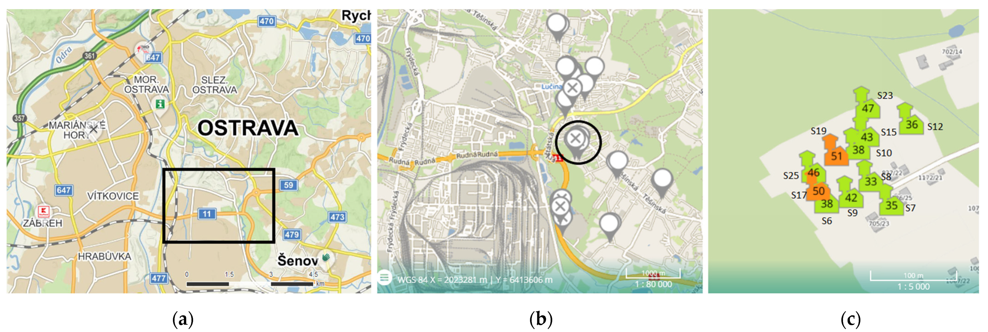
The sensor units in protective boxes were fitted to poles approximately 4 m above the ground level, and the distance of units from each other was roughly 10 m. The 11-unit cluster subject to evaluation occupied an area of approximately 70 m × 70 m (
Figure 1c) at one end of the urban Radvanice district in the south-eastern corner of the city of Ostrava, near smelter and ironworks facilities. The Radvanice district and surroundings have steadily recorded some of the worst air quality data in the Czech Republic from the beginning of regular air quality monitoring; recently, experiments focused on improving air quality have been conducted within the CLAIRO project.
The cluster presents one part of a large, 60-unit sensor network that continuously measures the area (up to 31 July 2021, more than 18 months) to evaluate the state and changes in air quality before and after application of the experimental measures. All sensor units contained a manufacturer-calibrated Alphasense OPC-N3 dust sensor and a Cairsens O3/NO2 sensor. In the initial phase of the measurements, and periodically throughout, the sensors were checked by reference measurements conducted on-site with a mobile air quality monitoring station. Based on the size of the area and location of the cluster, a homogeneous distribution of pollutants and, thus, similar behavior for all the sensors were expected.
Identification codes were assigned to sensor units that consisted of the letters S or Stc and numbers (S or Stc labelled with the same number mark the same sensor unit, depending on the automatic format of data exported from the database). Sensor locations, layout, and identification are given in
Figure 1c.
2.2. Particulate Matter Sensor—Alphasense OPC-N3
The Alphasense OPC-N3 sensors used (Alphasense, Ltd., Braintree, UK) were optical particle counters, certified according to ISO 9001:2015, which measure PM
1, PM
2,5, and PM
10 using a pre-programed internal distribution function, changes of which are rather cumbersome [
9]. Technical specifications [
10] are presented in
Table 1, and sensor appearance is presented in
Figure 2a.
The output of the Alphasense OPC-N3 sensor is values in µg/m3 which are logged in a Raspberry Pi control unit memory device and are regularly transferred as packages into the database.
Alphasense particulate matter sensors were calibrated against the FIDAS 200 optical particle counter (PALAS GMbH, Karlsruhe, Germany) as an equivalent method [
8]. As required by the standard, simultaneous measurements must last at least 24 h, and 5-min average values are used for comparison.
2.3. Ozone and Nitrous Oxide Combined Sensor Cairsens O3/NO2
The Cairsens (Envea, Poissy, France) combined sensor uses a 3-electrode electrochemical system (working, auxiliary, and reference electrodes) (Envea, France; appearance of the sensor shown in
Figure 2b). Gases of interest diffuse through a selective membrane towards the working electrode, and the signal produced is then directly proportional to the gas concentration (
Table 2). The sensor is equipped with a filter that reduces the influence of humidity. As part of the Cairsens sensor family, sensors can be used for individual measurements (data are stored in internal memory) or connected to clusters with their respective control units.
The producer calibrates the sensors, and the default output is produced in ppb (by volume), which needs further conversion to µg/m3 for air quality monitoring. For reference measurements, the AC32e chemiluminescence-based NO/NO2/NOX analyzer (Envea, Poissy, France) was used. Continuous parallel measurements were performed for 1 week, and 10-min average values were taken for statistical analysis.
2.4. Statistics
All statistical calculations were conducted with the StatPlus software (AnalystSoft, Inc., Walnut, CA, USA). The presented correlation coefficients were calculated as the Pearson correlation coefficient between two independent groups of variables (5-min averages for PM10 and 10-min averages for NO2) of both measurement methods along the same time period.
Validation factors were determined from long-term averages as a coefficient applied to sensor results to match with reference measurement results over the same time period.
Scatter plots were used for the visualization of the variable pairs. Reference method results were considered independent values, and sensory results as dependent variables for the comparisons. The scatter plots contain regression equations between independent and dependent variable sets and prediction lines based on them.
3. Results and Discussion
In the case of a 100% data yield, each of the sensors produced 8760 data points, corresponding to hourly averages and 105,120 5-min average values. The average yield of data throughout the monitored period was 97% for both PMx and NO
2 sensors. For statistical analysis purposes [
12] and measurement stability verification, data from 11 sensor units were used in the form of hourly averages calculated from 5-min average values stored in the database.
3.1. Suspended Particles PM10
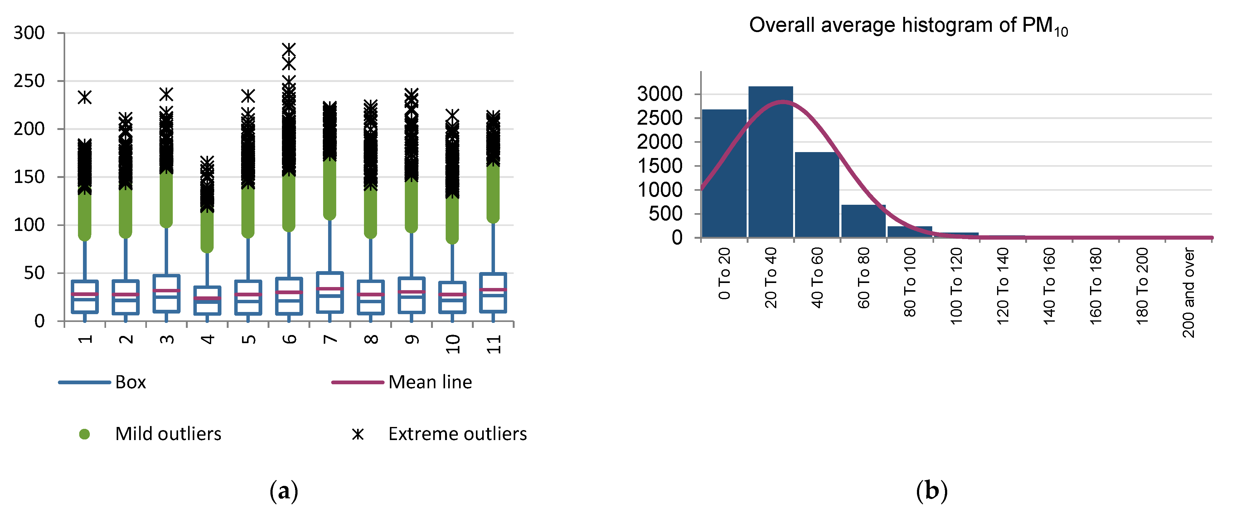
Table 3 presents the mean, median, and maximum values of all the sensors. The distribution of PM10 values is characteristic for ambient air, presenting a lower median than the arithmetic average and a skewness of 1.99. PM10 concentrations up to 40 µg/m
3 are most common in ambient air, as shown in
Figure 3; the values presented as outliers in the box plot are not, in fact, outlying extremes, but valid values of episodes of high concentrations that can occur infrequently. However, it must be emphasized that the measurements did not take place in a closed or controlled environment. Only sensor S8 produced values lower than the overall average throughout the measurement. Although the recorded concentration values and their changes were less dynamic and the variance was lower, the statistical analysis did not reveal outlying values produced by that sensor, or any significant effect on the overall average value.
The correlation matrix in
Table 4 lists all the relationships among the sensors in the group (55 values of correlation coefficients). The distribution of concentrations presented in
Figure 3 confirms the very good correlation of all sensors in the cluster. Due to the large number of results produced and the various conditions, the reliability of the sensors was tested for several concentration levels.
3.1.1. Low Concentration Level
A range of 1 to 10 µg/m
3 is considered a low concentration level of PM
10. The background level of PM
10 concentration in the Czech Republic generally exceeds 10 µg/m
3 [
13]. Reaching such a level of PM10 concentration is possible only in short periods of humid atmospheric conditions with precipitation, when the wet deposition of particles occurs. From the total number of 8580 hourly average values, only 856 values were below 10 µg/m
3.
Although the manufacturer states a lower limit of detection, measurements near the detection limit were impaired due to the lower sensitivity and higher imprecision. As suggested by the correlation matrix in
Table 5, the robustness of sensor measurements at low concentration levels is significantly lower, even in clustered parallel measurements, when compared to overall averages. The correlation matrix contains over 50% of very poor values. The sensors have proven unreliable for the monitoring of low concentrations of PM
10. Nevertheless, low concentration levels of particles in ambient air do not impose health risks, nor contribute to air pollution; therefore, the effects on the overall results of air quality monitoring are minimized.
3.1.2. Legislative Concentration Level Limit
The European Union states the concentration limit of PM10 in ambient air to be 50 µg/m
3 averaged over a 24-h measurement period, with a maximum of 35 episodes allowed to exceed the limit value [
14]. The most common concentration of suspended particles in the Ostrava region ranged between 10 and 100 µg/m
3. Therefore, measurement reliability is required to be very high at this concentration level. There were 7422 hourly concentration values collected in the database in total. As shown in the correlation matrices (
Table 5), correlation significantly increased in this range, showing that individual sensors behaved similarly and produced similar results that can be considered reproducible and reliable.
3.1.3. Very High Concentration Level
Episodes of extreme concentrations of suspended particles in the air exceeding the double value of the stated limit at 100 µg/m
3 regularly occur in the region. In the event of extremely unfavorable meteorological conditions, the PM
10 concentration can even reach up to an hourly average of 500 µg/m
3 [
13]. Sensors are not intended to be replacements of reference methods; therefore, regulation of the pollution sources based on their measurement is not possible. However, they should be capable of measurements at this concentration level.
Table 6 lists the recorded episodes of PM
10 concentration levels exceeding 100 µg/m
3 over the measurement period; the sensors did not indicate any false positive or false negative air quality situations. Although the correlation strength decreased in comparison to the midrange, the produced results are usable in general.
3.1.4. Comparison with Reference Measurements
Both sensory and reference measurement data were transferred into a database, which is accessible online on the website
www.airsens.eu (accessed on 10 May 2021). Raw measurement data were subject to correction that accounts for missing values (packets of data are mostly lost due to power shortages or problems with data transfer). Unpaired data were excluded to even pairs of data points in both groups. From the corrected 10-day average data, the validation factor was calculated as a coefficient for the sensor data to match the reference data (
Table 7).
Long-term data are presented in
Figure 4, which shows a comparison of reference measurements (FIDAS 200) and a sensor unit.
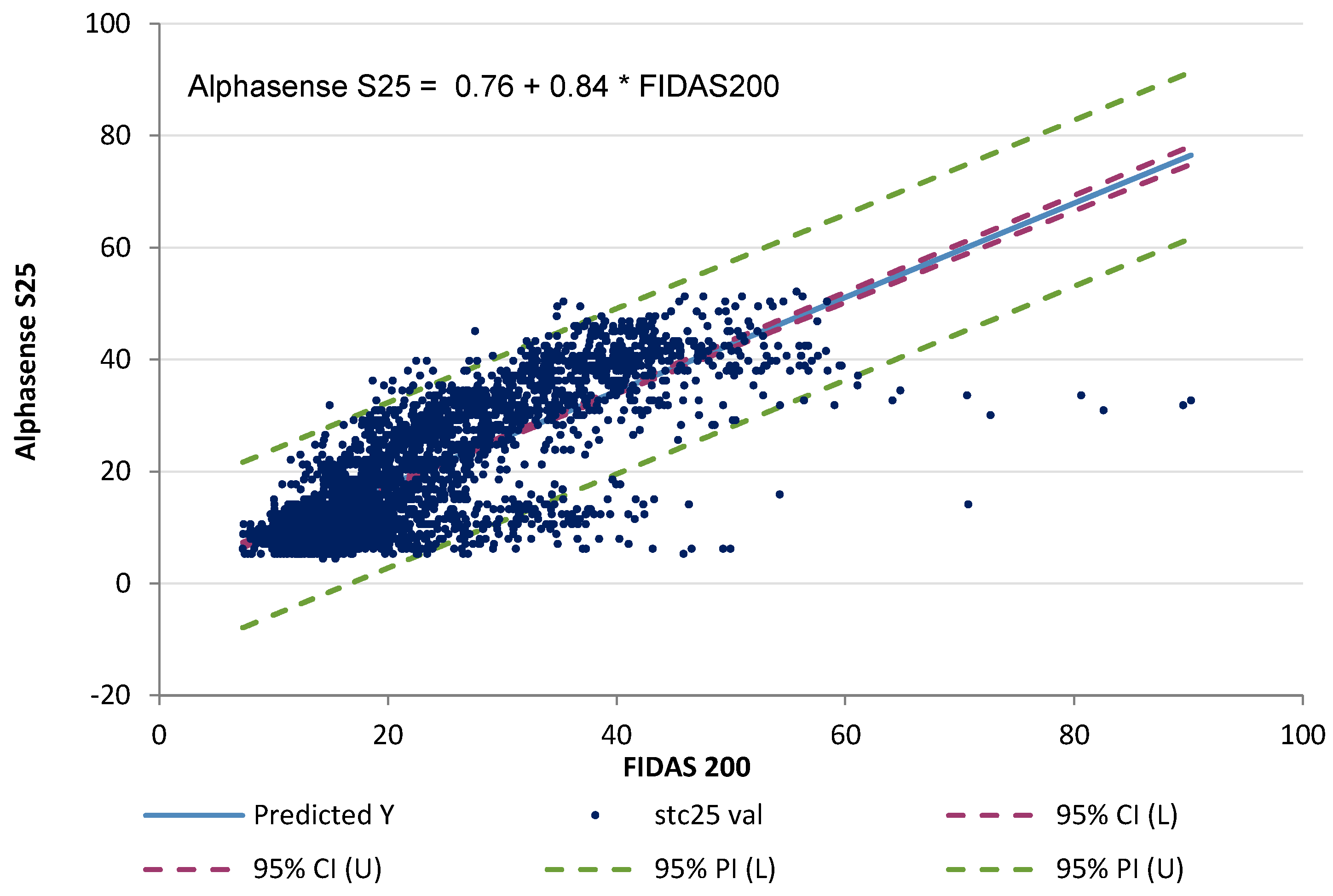
Sensor data after correction were multiplied by the validation coefficient, and the linear regression between datasets was calculated (
Figure 5). The correlation between the groups was strong, even though neither dataset was corrected for measurement conditions (relative humidity, temperature, etc.) that can lead to the over- or underestimation of sensor-measured values in comparison to the reference instrument [
15,
16].
All the PM10 sensor units have been operating continuously for at least 18 months, including two winter seasons with no significant deterioration of measurement quality recorded so far.
3.2. Nitrous Oxide NO2
3.2.1. Sensory Measurements
Cairsens sensors provide the output of NO
2 concentration in ppb units; therefore, conversion to µg/m
3 is necessary before further operation. Statistical calculations were carried out with converted values using a factor of 1.882 (25 °C, 101.325 kPa). An overview of the measured concentrations is presented in
Table 8.
Similarly to the PM
10 sensors, the group contained one sensor that provided lower values (S7) than the rest of the group; however, the statistical analysis did not prove the values to be outlying, so the results were considered valid and used further.
Table 9 presents the correlation matrix among the sensors; in
Figure 6, the distribution of the measured values is shown.
The correlations among some of the sensors are strong (35% of the coefficient values in the matrix are higher than 0.7), with most being low to moderate. Considering that there is no source of NO2 in the surroundings of the cluster location, such as congested roads or large combustion sources, the measured NO2 concentration was more stable than the PM10 concentration. The shift in concentration towards lower values (below 10 µg/m3) is characteristic of NO2.
3.2.2. Comparison with Reference Measurements
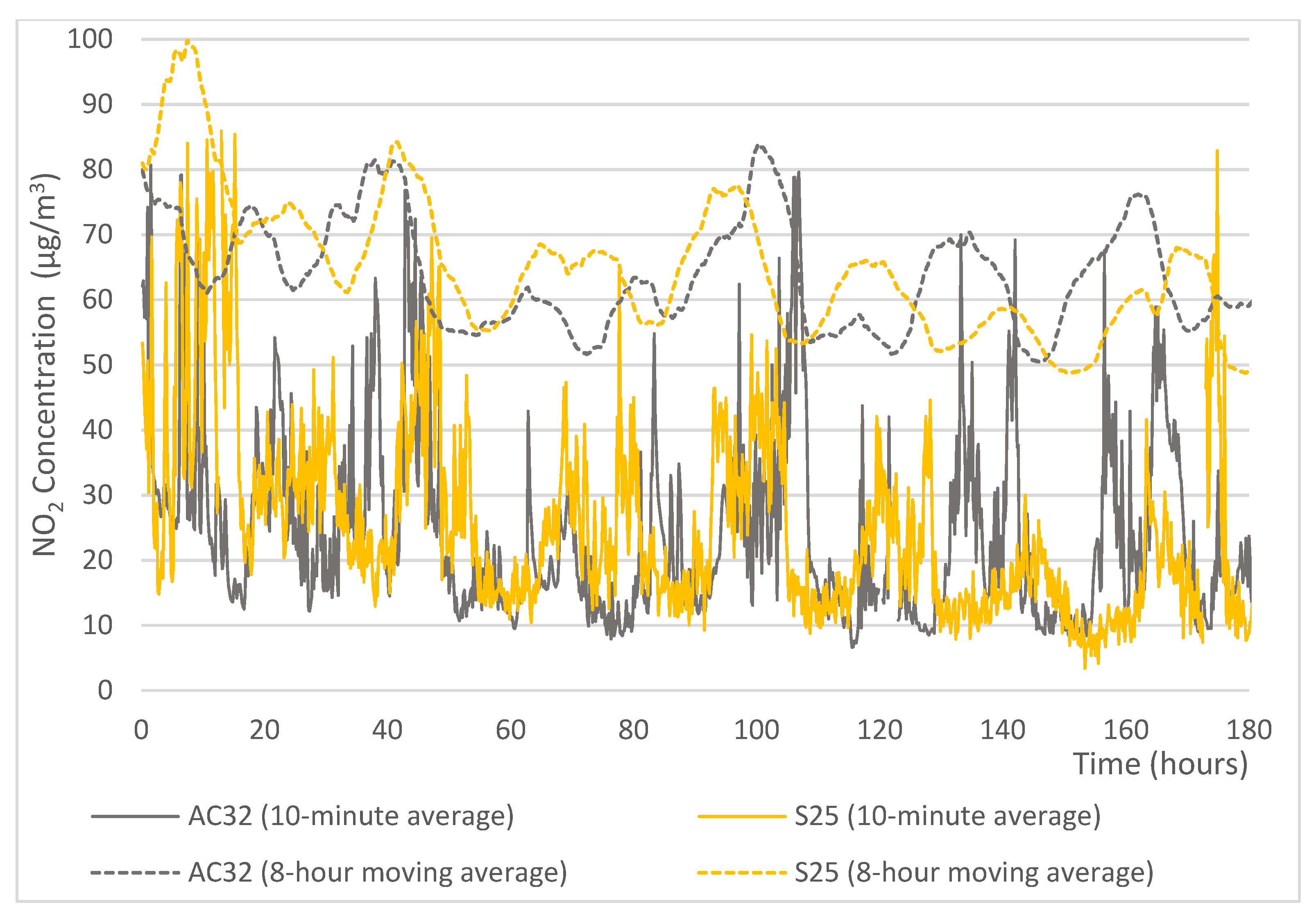
Sensory and reference measurement datasets underwent identical procedures (exclusion of unpaired values, calculation of validation coefficient using 10-day average, and linear regression), revealing that the linear correlation among the sensory data and reference instruments was very poor (
Table 10,
Figure 7), even though average values were similar and long-term timelines showed very similar trends (
Figure 8).
The outputs of the NO
2 sensors were not corrected for any influences or interferences. Highly improved correlations between reference and sensory measurements are reported in studies after the introduction of correction functions (mainly correcting for influences of temperature and relative humidity, or duration of the operation period), using non-linear regression methods or artificial neural networks [
17,
18,
19]. Although correlation based on linear regression methods is poor, all the studies cited mention the consistency of concentration trends in averaged periods over several minutes to hours. Similarly, differences between calibrations in controlled laboratory conditions and field measurements of ambient air are commonly described [
19,
20,
21,
22,
23,
24]. Measurements of the combined Cairsens sensors were based on reactions of oxidizing gases, i.e., the sum of present NO
2, ozone, and interferences. In combined sensors, the electric signal from the sensing layer is always mathematically processed to produce NO
2 and ozone concentrations as the output. The computation can take place in the electronics of the dual-channel sensor assembly, or a single-channel output presents an input for the computation cascade in the data processing step.
3.3. Sensor Data-Based Network
Attempts to obtain additional and more detailed air quality data than may be supplied by the official air quality monitoring stations have been made ever since the start of AQM. Due to the price of the sensors, networks covering various areas can be easily established.
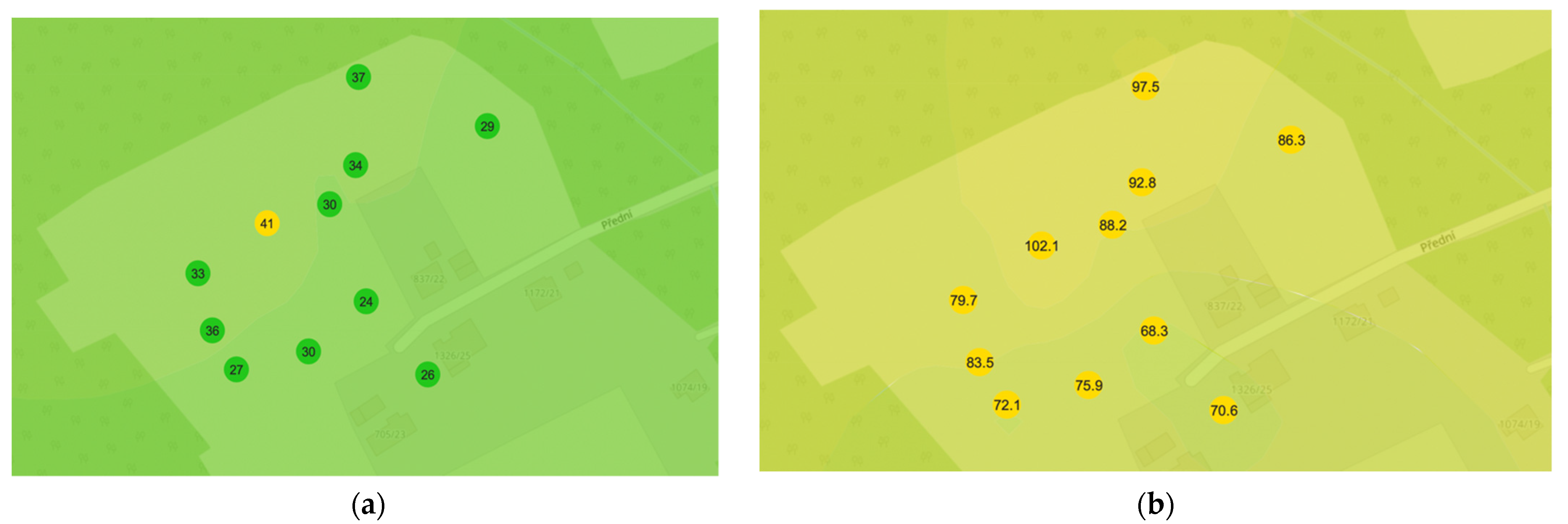
In our case, sensors were used as a source of complementary high-density data, based on the deployment of the sensor network. The data stored in the database could be visualized on a map, and the evolution and partial prediction of air pollution is possible.
Figure 9 shows a model which is already in use with the data stored in the database that adds a colored layer over the map of the locations monitored by sensors, showing the current situation. In such cases, trends and changes in concentration values, as well as spatial and temporal resolution, are preferred over measurement precision and accuracy.
4. Conclusions
The purpose of the study was to verify whether it is possible to continuously use optical PMx and electrochemical NO2 sensors for 12 months, and to what extent the original calibration/setup is useful for the whole measurement period. Annual measurements proved that the sensor system arranged in a network is quite robust and stable. Although there were variations in the individual sensors for both PM10 and NO2, there were no significant differences in the cluster.
In the case of PM10, some of the sensors revealed slower responses to changes in concentration (S4, S8, S25), although one of the sensors responded significantly faster (S17). Finally, all the sensor-produced data had very similar basic statistical characteristics, such as the mean, median, and maximum measured values. Thus, in the long term, they provide identical air quality data. The correlations show very good agreement among the individual sensors in the range of normal and high PM10 concentrations. High agreement only decreases for low concentration levels, which scarcely occur and are not problematic from an air pollution and health risk point of view. Based on our results, Alphasense OPC-N3 sensors can also be utilized as single indicators in addition to their use in a network.
The characteristics of the NO2 sensory measurements were poor using linear regression methods. Poor statistical parameters and correlations can be improved with the use of correction functions and/or more advanced data analysis methods. Dispersion of the measured values (dynamics) varied among the sensors, but basic parameters (maxima and average values) of individual sensors datasets were similar, as well as their trends and changes during the monitoring period. It can be summarized that differences among sensors can be compensated for with multiple units deployed in the cluster for parallel measurements.
For both types of sensors, it can be concluded that they are currently not suitable as a substitute for reference techniques, especially if one sensor is intended to replace one device.
However, the sensors are very suitable for monitoring trends and concentration changes in monitored pollutants when deployed in clusters and networks that provide high spatial and temporal resolution. The long-term usability was also proved by annual measurements. Although none of the sensor devices needed replacing, the quality of each individual device is important for both data quality and unit usability.
Author Contributions
Conceptualization, J.B., O.B. and P.B.; methodology, J.B.; software, J.B. and O.B.; validation, P.M., P.B. and O.B.; formal analysis, P.M.; investigation, P.M., P.B. and O.B.; resources, P.M.; data curation, O.B.; writing—original draft preparation, J.B.; writing—review and editing, P.B.; visualization, O.B.; supervision, J.B.; project administration, J.B.; funding acquisition, J.B. All authors have read and agreed to the published version of the manuscript.
Funding
This research was funded by the Ministry of Education, Youth and Sports of the Czech Republic in the framework of the National Sustainability by ERDF/ESF, grant number CZ.02.1.01/0.0/0.0/18_069/0010049 “Research on the identification of combustion of unsuitable fuels and systems of self-diagnostics of boilers combustion solid fuels for domestic heating”.
Acknowledgments
Authors would like to thank the UIA03-123 CLAIRO (CLear AIR and Climate Adaptation in Ostrava and other cities) project, co-financed by the European Regional Development Fund for the possibility to build and deploy the sensor network for ambient air quality monitoring and data collection.
Conflicts of Interest
The authors declare no conflict of interest. The funders had no role in the design of the study; in the collection, analyses, or interpretation of data; in the writing of the manuscript, or in the decision to publish the results.
References
- Gerboles, M.; Spinelle, L.; Borowiak, A. Measuring Air Pollution with Low-Cost Sensors. Available online: https://core.ac.uk/reader/132627234 (accessed on 28 May 2021).
- Lewis, A.C.; von Schneidemesser, E.; Peltier, R.E. (Eds.) Low-Cost Sensors for the Measurement of Atmospheric Composition: Overview of Topic and Future Applications; WMO-No.1215; World Meteorological Organization: Geneva, Switzerland, 2018; ISBN 978-92-63-11215-6. [Google Scholar]
- Bauerová, P.; Šindelářová, A.; Rychlík, Š.; Novák, Z.; Keder, J. Low-Cost Air Quality Sensors: One-Year Field Comparative Measurement of Different Gas Sensors and Particle Counters with Reference Monitors at Tušimice Observatory. Atmosphere 2020, 11, 492. [Google Scholar] [CrossRef]
- Lewis, A.; Edwards, P. Validate Personal Air-Pollution Sensors. Nature 2016, 535, 29–31. [Google Scholar] [CrossRef] [PubMed] [Green Version]
- Spinelle, L.; Gerboles, M.; Villani, M.G.; Aleixandre, M.; Bonavitacola, F. Field Calibration of a Cluster of Low-Cost Available Sensors for Air Quality Monitoring. Part A: Ozone and Nitrogen Dioxide. Sens. Actuators B Chem. 2015, 215, 249–257. [Google Scholar] [CrossRef]
- Spinelle, L.; Gerboles, M.; Villani, M.G.; Aleixandre, M.; Bonavitacola, F. Field Calibration of a Cluster of Low-Cost Commercially Available Sensors for Air Quality Monitoring. Part B: NO, CO and CO2. Sens. Actuators B Chem. 2017, 238, 706–715. [Google Scholar] [CrossRef]
- Kelly, K.E.; Whitaker, J.; Petty, A.; Widmer, C.; Dybwad, A.; Sleeth, D.; Martin, R.; Butterfield, A. Ambient and Laboratory Evaluation of a Low-Cost Particulate Matter Sensor. Environ. Pollut. 2017, 221, 491–500. [Google Scholar] [CrossRef] [PubMed]
- European Standards. EN 12341:2014 Ambient Air–Standard Gravimetric Measurement Method for the Determination of the PM10 or PM2.5 Mass Concentration of Suspended Particulate Matter; CEN–European Committee for Standardization: Brussels, Belgium, 2014. [Google Scholar]
- Görner, P.; Wrobel, R.; Mička, V.; Škoda, V.; Denis, J.; Fabriès, J.-F. Study of Fifteen Respirable Aerosol Samplers Used in Occupational Hygiene. Ann. Occup. Hyg. 2001, 45, 43–54. [Google Scholar] [CrossRef]
- Air Quality Sensors Field Evaluation. Available online: http://www.aqmd.gov/aq-spec/evaluations/field (accessed on 30 November 2020).
- Cairsens® O3/NO2 |Micro-Sensors| Ambient. Available online: https://www.envea.global/s/ambient-en/micro-sensors-a/cairsens-o3-no2/ (accessed on 31 May 2021).
- Meloun, M.; Militký, J. Kompendium Statistického Zpracování Dat, 3rd ed.; Karolinum: Praha, Czech Republic, 2012; ISBN 978-80-246-2196-8. [Google Scholar]
- ISKO. Tabelární Ročenky. Available online: https://www.chmi.cz/files/portal/docs/uoco/isko/tab_roc/tab_roc_CZ.html (accessed on 24 May 2021).
- The European Parliament and the Council of the European Uniondirective. 2008/50/EC of the European Parliament and of the Council of 21 May 2008 on Ambient Air Quality and Cleaner Air for Europe; Available online: https://eur-lex.europa.eu/eli/dir/2008/50/oj (accessed on 12 August 2021).
- Kaliszewski, M.; Włodarski, M.; Młyńczak, J.; Kopczyński, K. Comparison of Low-Cost Particulate Matter Sensors for Indoor Air Monitoring during COVID-19 Lockdown. Sensors 2020, 20, 7290. [Google Scholar] [CrossRef] [PubMed]
- Badura, M.; Batog, P.; Drzeniecka-Osiadacz, A.; Modzel, P. Evaluation of Low-Cost Sensors for Ambient PM2.5 Monitoring. J. Sens. 2018, 2018, e5096540. [Google Scholar] [CrossRef] [Green Version]
- Munir, S.; Mayfield, M.; Coca, D.; Jubb, S.; Osammor, O. Analysing the Performance of Low-Cost Air Quality Sensors, Their Drivers, Relative Benefits and Calibration in Cities—A Case Study in Sheffield. Environ. Monit. Assess. 2019. [Google Scholar] [CrossRef] [PubMed] [Green Version]
- Clougherty, J.E.; Kheirbek, I.; Eisl, H.M.; Ross, Z.; Pezeshki, G.; Gorczynski, J.E.; Johnson, S.; Markowitz, S.; Kass, D.; Matte, T. Intra-Urban Spatial Variability in Wintertime Street-Level Concentrations of Multiple Combustion-Related Air Pollutants: The New York City Community Air Survey (NYCCAS). J. Expo. Sci. Environ. Epidemiol. 2013, 23, 232–240. [Google Scholar] [CrossRef] [PubMed]
- Castell, N.; Dauge, F.R.; Schneider, P.; Vogt, M.; Lerner, U.; Fishbain, B.; Broday, D.; Bartonova, A. Can Commercial Low-Cost Sensor Platforms Contribute to Air Quality Monitoring and Exposure Estimates? Environ. Int. 2017, 99, 293–302. [Google Scholar] [CrossRef] [PubMed]
- Castell, N.; Viana, M.; Minguillón, M.C.; Guerreiro, C.; Querol, X. Real-World Application of New Sensor Technologies for Air Quality Monitoring ETC/ACM Technical Paper 2013/16; The European Topic Centre on Air Pollution and Climate Change Mitigation: Bilthoven, The Netherlands, 2013; p. 34. [Google Scholar]
- Jiao, W.; Hagler, G.; Williams, R.; Sharpe, R.; Brown, R.; Garver, D.; Judge, R.; Caudill, M.; Rickard, J.; Davis, M.; et al. Community Air Sensor Network (CAIRSENSE) Project: Evaluation of Low-Cost Sensor Performance in a Suburban Environment in the Southeastern United States. Atmos. Meas. Tech. 2016, 9, 5281–5292. [Google Scholar] [CrossRef] [PubMed] [Green Version]
- Sun, L.; Wong, K.C.; Wei, P.; Ye, S.; Huang, H.; Yang, F.; Westerdahl, D.; Louie, P.K.K.; Luk, C.W.Y.; Ning, Z. Development and Application of a Next Generation Air Sensor Network for the Hong Kong Marathon 2015 Air Quality Monitoring. Sensors 2016, 16, 211. [Google Scholar] [CrossRef] [PubMed]
- Mijling, B.; Jiang, Q.; de Jonge, D.; Bocconi, S. Field Calibration of Electrochemical NO2 Sensors in a Citizen Science Context. Atmos. Meas. Tech. 2018, 11, 1297–1312. [Google Scholar] [CrossRef] [Green Version]
- Sales-Lérida, D.; Bello, A.J.; Sánchez-Alzola, A.; Martínez-Jiménez, P.M. An Approximation for Metal-Oxide Sensor Calibration for Air Quality Monitoring Using Multivariable Statistical Analysis. Sensors 2021, 21, 4781. [Google Scholar] [CrossRef] [PubMed]
Figure 1.
Sensor network location: (a) monitored area within the city of Ostrava; (b) overview of the city quarters and the deployed sensor network; and (c) detail of the evaluated cluster of sensor units, their identification, and visualization of measured values.
Figure 1.
Sensor network location: (a) monitored area within the city of Ostrava; (b) overview of the city quarters and the deployed sensor network; and (c) detail of the evaluated cluster of sensor units, their identification, and visualization of measured values.
Figure 2.
External view of the (a) Alphasense OPC-N3 sensor, approximate dimensions of 75 × 64 × 60 mm and (b) the Cairsens© sensor, approximate dimensions of 65 mm length and 33 mm diameter, inserted view of the bottom part with air intake.
Figure 2.
External view of the (a) Alphasense OPC-N3 sensor, approximate dimensions of 75 × 64 × 60 mm and (b) the Cairsens© sensor, approximate dimensions of 65 mm length and 33 mm diameter, inserted view of the bottom part with air intake.
Figure 3.
Distribution of PM10 values recorded throughout the year-long measurements: (a) box plot for individual sensors in the cluster and (b) histogram of hourly averages (overall averaged values of all sensors).
Figure 3.
Distribution of PM10 values recorded throughout the year-long measurements: (a) box plot for individual sensors in the cluster and (b) histogram of hourly averages (overall averaged values of all sensors).
Figure 4.
Example of parallel 10-day measurements of PM10 values measured by a sensor and a reference instrument (FIDAS 200); moving average values were offset by 40 µg/m3.
Figure 4.
Example of parallel 10-day measurements of PM10 values measured by a sensor and a reference instrument (FIDAS 200); moving average values were offset by 40 µg/m3.
Figure 5.
Linear regression plot of reference measurement results (FIDAS 200). Measured and predicted sensory values according to regression equation are presented in the plot.
Figure 5.
Linear regression plot of reference measurement results (FIDAS 200). Measured and predicted sensory values according to regression equation are presented in the plot.
Figure 6.
Distribution of NO2 values throughout the year-long measurement: (a) box plot for individual sensors and (b) histogram of hourly averages (overall averaged values of all sensors).
Figure 6.
Distribution of NO2 values throughout the year-long measurement: (a) box plot for individual sensors and (b) histogram of hourly averages (overall averaged values of all sensors).
Figure 7.
Regression plot of reference (AC32) vs. sensor (S25) datasets.
Figure 7.
Regression plot of reference (AC32) vs. sensor (S25) datasets.
Figure 8.
Comparison of reference (AC32) and sensor (S25) data for NO2 over the 7-day measurement; moving average values are offset by 40 µg/m3.
Figure 8.
Comparison of reference (AC32) and sensor (S25) data for NO2 over the 7-day measurement; moving average values are offset by 40 µg/m3.
Figure 9.
Visualized situation of the air quality based on NO2 sensor data: (a) low average concentrations in the area and (b) elevated concentrations of NO2.
Figure 9.
Visualized situation of the air quality based on NO2 sensor data: (a) low average concentrations in the area and (b) elevated concentrations of NO2.
Table 1.
Technical specifications of the Alphasense OPC-N3 sensor.
Table 1.
Technical specifications of the Alphasense OPC-N3 sensor.
| Sensed Matter | PMx |
|---|
| Measured particle size | 0.35–40 µm |
| Number of size classes | 24 |
| Limit of detection | <1 µg/m3 |
| Measurement range | 0–2000 µg/m3 |
| Sensitivity | <1 µg/m3 |
Table 2.
Technical specifications of the Cairsens© NO
2/O
3 sensor [
11].
Table 2.
Technical specifications of the Cairsens© NO
2/O
3 sensor [
11].
| Sensed Matter | NO2/O3 |
|---|
| Limit of detection | 20 ppb (vol) |
| Measurement range | 0–250 ppb |
| Sensitivity | 1 ppb3 |
| Uncertainty | <30% |
| Interferences | Chlorine gas |
Table 3.
Hourly average values of particulate matter recorded over the 1-year monitoring period.
Table 3.
Hourly average values of particulate matter recorded over the 1-year monitoring period.
| | | PM10 (µg/m3) | |
|---|
| Sensor No. | Mean | Median | Maximum |
|---|
| S4 | 28.09 | 22.45 | 233.09 |
| S6 | 27.72 | 21.54 | 210.69 |
| S7 | 31.84 | 25.09 | 236.38 |
| S8 | 23.87 | 19.98 | 165.32 |
| S10 | 27.84 | 20.46 | 234.66 |
| S12 | 30.04 | 21.12 | 282.82 |
| S15 | 33.84 | 26.11 | 222.28 |
| S17 | 27.87 | 20.49 | 223.86 |
| S19 | 30.57 | 25.11 | 235.86 |
| S23 | 27.72 | 21.55 | 214.19 |
| S25 | 32.76 | 26.72 | 212.88 |
Table 4.
Correlation matrix of all PM10 data recorded by all sensors.
Table 4.
Correlation matrix of all PM10 data recorded by all sensors.
| R | S4 | S6 | S7 | S8 | S10 | S12 | S15 | S17 | S19 | S23 | S25 |
|---|
| S4 | 1.00 | | | | | | | | | | |
| S6 | 0.69 | 1.00 | | | | | | | | | |
| S7 | 0.71 | 0.91 | 1.00 | | | | | | | | |
| S8 | 0.64 | 0.85 | 0.86 | 1.00 | | | | | | | |
| S10 | 0.63 | 0.75 | 0.82 | 0.68 | 1.00 | | | | | | |
| S12 | 0.62 | 0.75 | 0.81 | 0.66 | 0.94 | 1.00 | | | | | |
| S15 | 0.78 | 0.73 | 0.75 | 0.67 | 0.64 | 0.65 | 1.00 | | | | |
| S17 | 0.61 | 0.70 | 0.76 | 0.59 | 0.86 | 0.89 | 0.61 | 1.00 | | | |
| S19 | 0.67 | 0.88 | 0.87 | 0.85 | 0.69 | 0.70 | 0.72 | 0.72 | 1.00 | | |
| S23 | 0.83 | 0.73 | 0.75 | 0.72 | 0.62 | 0.62 | 0.75 | 0.61 | 0.74 | 1.00 | |
| S25 | 0.70 | 0.74 | 0.77 | 0.69 | 0.64 | 0.65 | 0.81 | 0.60 | 0.72 | 0.82 | 1.00 |
Table 5.
Overview of correlation matrices among PM10 sensors.
Table 5.
Overview of correlation matrices among PM10 sensors.
R
Absolute Value | Strength of Correlation | Overall | Low
Concentrations (<10 µg/m3) | Legislation Limit
(10–100 µg/m3) | High Concentrations
(>100 µg/m3) |
|---|
| 0.90–1.00 | Very high | 2 | - | 14 | 1 |
| 0.70–0.90 | High | 32 | 7 | 41 | 19 |
| 0.50–0.70 | Moderate | 21 | 7 | - | 12 |
| 0.30–0.50 | Low | - | 16 | - | 23 |
| 0.00–0.30 | Little, if any | - | 25 | - | - |
| Number of values in the group | | 8580 | 856 | 7422 | 302 |
| Maximum R | | 0.94 | 0.85 | 0.97 | 0.99 |
| Minimum R | | 0.59 | 0.03 | 0.75 | 0.3 |
Table 6.
Monthly overview of high concentration cases (PM10 concentration exceeding an hourly average of 100 µg/m3).
Table 6.
Monthly overview of high concentration cases (PM10 concentration exceeding an hourly average of 100 µg/m3).
| Month | Number of Episodes |
|---|
| October 2019 | 90 |
| November 2019 | 107 |
| December 2019 | 18 |
| January 2020 | 22 |
| February 2020 | 8 |
| March 2020 | 46 |
| April 2020 | 9 |
| May 2020 | 2 |
Table 7.
Data used to determine the validation factor (sensor unit no. S25).
Table 7.
Data used to determine the validation factor (sensor unit no. S25).
| PM10 (µg/m3) | Alphasense
S-25 | Reference
FIDAS 200 | Validation
Factor | Correlation
Coefficient R |
|---|
| 24-h average | 23.61 | 23.67 | | |
| 72-h average | 25.33 | 23.46 | | |
| 240-h average | 23.94 | 23.93 | 1.014 | 0.78 |
Table 8.
Average hourly values of NO2 concentration recorded over the 1-year monitoring period.
Table 8.
Average hourly values of NO2 concentration recorded over the 1-year monitoring period.
| | | NO2 (µg/m3) | |
|---|
| Sensor No. | Mean | Median | Maximum |
|---|
| S4 | 22.8 | 15.3 | 264.0 |
| S6 | 22.5 | 14.6 | 211.9 |
| S7 | 21.6 | 15.0 | 269.2 |
| S8 | 25.2 | 16.3 | 270.8 |
| S10 | 25.5 | 18.8 | 190.1 |
| S12 | 24.5 | 17.9 | 202.6 |
| S15 | 23.1 | 16.5 | 199.4 |
| S17 | 23.6 | 15.4 | 253.3 |
| S19 | 24.3 | 16.0 | 233.2 |
| S23 | 23.2 | 15.7 | 217.3 |
| S25 | 22.3 | 15.7 | 173.1 |
Table 9.
Correlation matrix of sensor-measured NO2 concentrations.
Table 9.
Correlation matrix of sensor-measured NO2 concentrations.
| R | S4 | S6 | S7 | S8 | S10 | S12 | S15 | S17 | S19 | S23 | S25 |
|---|
| S4 | 1.00 | | | | | | | | | | |
| S6 | 0.46 | 1.00 | | | | | | | | | |
| S7 | 0.51 | 0.77 | 1.00 | | | | | | | | |
| S8 | 0.46 | 0.91 | 0.78 | 1.00 | | | | | | | |
| S10 | 0.44 | 0.74 | 0.91 | 0.77 | 1.00 | | | | | | |
| S12 | 0.46 | 0.73 | 0.89 | 0.78 | 0.99 | 1.00 | | | | | |
| S15 | 0.79 | 0.43 | 0.50 | 0.51 | 0.44 | 0.48 | 1.00 | | | | |
| S17 | 0.55 | 0.62 | 0.80 | 0.63 | 0.86 | 0.86 | 0.47 | 1.00 | | | |
| S19 | 0.55 | 0.88 | 0.70 | 0.90 | 0.67 | 0.69 | 0.45 | 0.71 | 1.00 | | |
| S23 | 0.69 | 0.30 | 0.37 | 0.35 | 0.33 | 0.35 | 0.65 | 0.44 | 0.41 | 1.00 | |
| S25 | 0.58 | 0.35 | 0.43 | 0.40 | 0.39 | 0.41 | 0.73 | 0.38 | 0.31 | 0.87 | 1.00 |
Table 10.
Data used to determine the validation factor (NO2, sensor unit no. S25).
Table 10.
Data used to determine the validation factor (NO2, sensor unit no. S25).
| NO2 (µg/m3) | Cairsens | Reference
AC32e | Validation
Factor | Correlation
Coefficient R |
|---|
| 24-h average | 24.46 | 24.44 | - | - |
| 72-h average | 23.38 | 22.78 | - | - |
| 240-h average | 24.63 | 24.62 | 0.97 | 0.28 |
| Publisher’s Note: MDPI stays neutral with regard to jurisdictional claims in published maps and institutional affiliations. |
© 2021 by the authors. Licensee MDPI, Basel, Switzerland. This article is an open access article distributed under the terms and conditions of the Creative Commons Attribution (CC BY) license (https://creativecommons.org/licenses/by/4.0/).


