
COMSOL Modeling of Heat Transfer in SVE Process


1
School of Automation Science and Electrical Engineering, Beihang University, Beijing 100191, China
2
School of Mechanical Engineering, Inner Mongolia University of Science and Technology, Baotou 014030, China
3
Engineering Training Centre, Beihang University, Beijing 100191, China
*
Author to whom correspondence should be addressed.
Environments 2022, 9(5), 58; https://0-doi-org.brum.beds.ac.uk/10.3390/environments9050058
Submission received: 26 January 2022
/
Revised: 21 April 2022
/
Accepted: 7 May 2022
/
Published: 11 May 2022
(This article belongs to the Topic Organic Pollution in Soil and Groundwater)
Abstract
:Non aqueous phase liquid (NAPL) pollution exists in porous media such as soil. SVE technology can be used to remove this pollution in soil. However, few domestic and international studies have paid attention to the changes of soil temperature in the field, which we believe can be useful information to optimize the layout of heating wells. In this research we established partial differential equations of soil heat transfer using the COMSOL multi-field coupling tool to simulate the field distribution of the change in soil internal temperature in the process of SVE to obtain the change of effective heating area with time under certain initial heating conditions. At the same time, we used liquid ethylbenzene to represent NAPL pollutants, and designed a simulation of soil temperature field distribution under the movement of liquid ethylbenzene under external pressure. It was found that under the action of Darcy’s velocity field, the utilization efficiency of the SVE system for the heat source was significantly improved, that is, the temperature distribution of the soil was more uniform. However, the temperature of the heated area increased slowly because the extraction well took away the heat energy. The heat source power should be increased or prolonged to improve the effect of Darcy’s field. Through a coupled simulation, we obtained a variation relationship of the soil temperature field in 1800 min under the action of one extraction well and four heating wells. These data will provide the basis for our next step in designing an algorithm to optimize the distribution of heating wells.
1. Introduction
Soil pollution of industrial land has caused great pressure on the ecosystem. Compared with other pollution, such as water pollution, NAPL pollution can exist in soil for many years, and its soluble components gradually penetrate and diffuse into groundwater along the soil layer, forming deep-seated and more lasting pollution. Many studies have been conducted on the transport and distribution of NAPL. For example, an electrical imaging method and a soil radon deficiency survey have been used to evaluate the pollution degree of NAPL in aeration zones [1,2], and nanotechnology and biotechnology have been used to study the concentration and transfer trend of NAPL [3,4]. In addition, some researchers have also studied the repair process of NAPL pollution with surfactants [5,6,7,8] and the effects of temperature and other factors on the diffusion rate of NAPL in groundwater and other media [9,10,11,12].
Since 1990s, soil vapor extraction (SVE) has been used in industry to remove the pollution caused by NAPLs. In this field, many scholars have established SVE models to simulate mass transfer and other processes in the SVE method [13,14,15,16,17]. Other scholars have focused on the effects of gas flow rate [18], water level fluctuation [19,20] and initial organic concentration [21] on pollutant migration efficiency in gas phase extraction. In addition, some scholars have used SVE combined with bioremediation and other remediation methods to remove NAPLs pollutants in soil [22,23]. However, domestic and international scholars have paid more attention to the influence of conditions and removal results of SVE technology to remove pollutants, while few have paid attention to the energy consumption cost of SVE removal of pollutants, which is the reason why SVE technology has not been used on a large scale in China.
Optimizing heater well distribution is an effective way to reduce the cost of SVE. Considering that heating temperature is an important factor for the removal of volatile organic compounds, and some organic compounds can be oxidized into water and carbon dioxide with SVE technology, we established a heat transfer model for the SVE process, aiming to obtain the soil temperature during the SVE heating process through simulation. This study focuses on changes of the soil temperature field caused by heating wells as important reference information for optimizing the distribution of heating wells.
COMSOL is a powerful multi physical field simulation tool. It integrates many self-developed solution modules and allows users to add control equations to the model according to their needs. Compared with classical mechanical analysis software, such as ANSYS, it can also effectively converge in multi-physics coupling simulation.
In this paper, the COMSOL multi field coupling tool and other calculation tools are used to establish partial differential equations, materialize conceptual units, and simulate the change of the soil temperature field under a multi-field coupling state, based on porous medium heat transfer and Darcy’s law, to provide a reference for removing industrial land pollution by SVE Technology.
The other parts of this paper are as follows. The second part introduces the relevant principles of porous media heat transfer and Darcy’s law, the third part introduces the simulation results of porous media heat transfer, the fourth part introduces the simulation results of the COMSOL model after adding the Darcy velocity field, and the fifth part is the conclusion.
2. Materials and Methods
2.1. Heat Transfer Model of Porous Media
2.1.1. Model Building
In a simulation, time and temperature should be given priority because they have the greatest impact on the removal result of soil pollution, and the impact of exhaust flow from the removal effect of pollutants is less than that of the concentration of pollutants themselves. Therefore, the model can be simplified to focus on analysis of the temperature field distribution of soil with time under a given initial condition.
A heat transfer model of porous media is shown in the Figure 1 below:
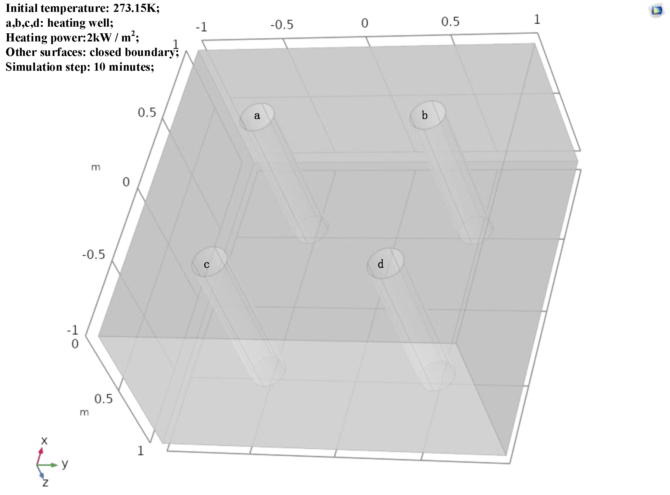
As showed in the figure, the model is a rectangle of (2 × 2 × 1) m3. Assuming that the upper boundary of the model is the ground, four heat source areas with a diameter of 1dm and a depth of 1m are symmetrically distributed with four positions {(0.5, 0.5), (0.5, −0.5), (−0.5, 0.5), (−0.5, −0.5)} on the xoy plane of the model as the center. The heat source is a boundary heat source, the constant heating power is 2 kW/m2, and the heat distribution in the heat source area is uniform. Therefore, the heat source medium does not need to be considered. The main solid medium in porous media is soil and the fluid medium is ethylbenzene. The specific properties are introduced later in this paper. The grid division is controlled by the physical field, and the division result is as follows.
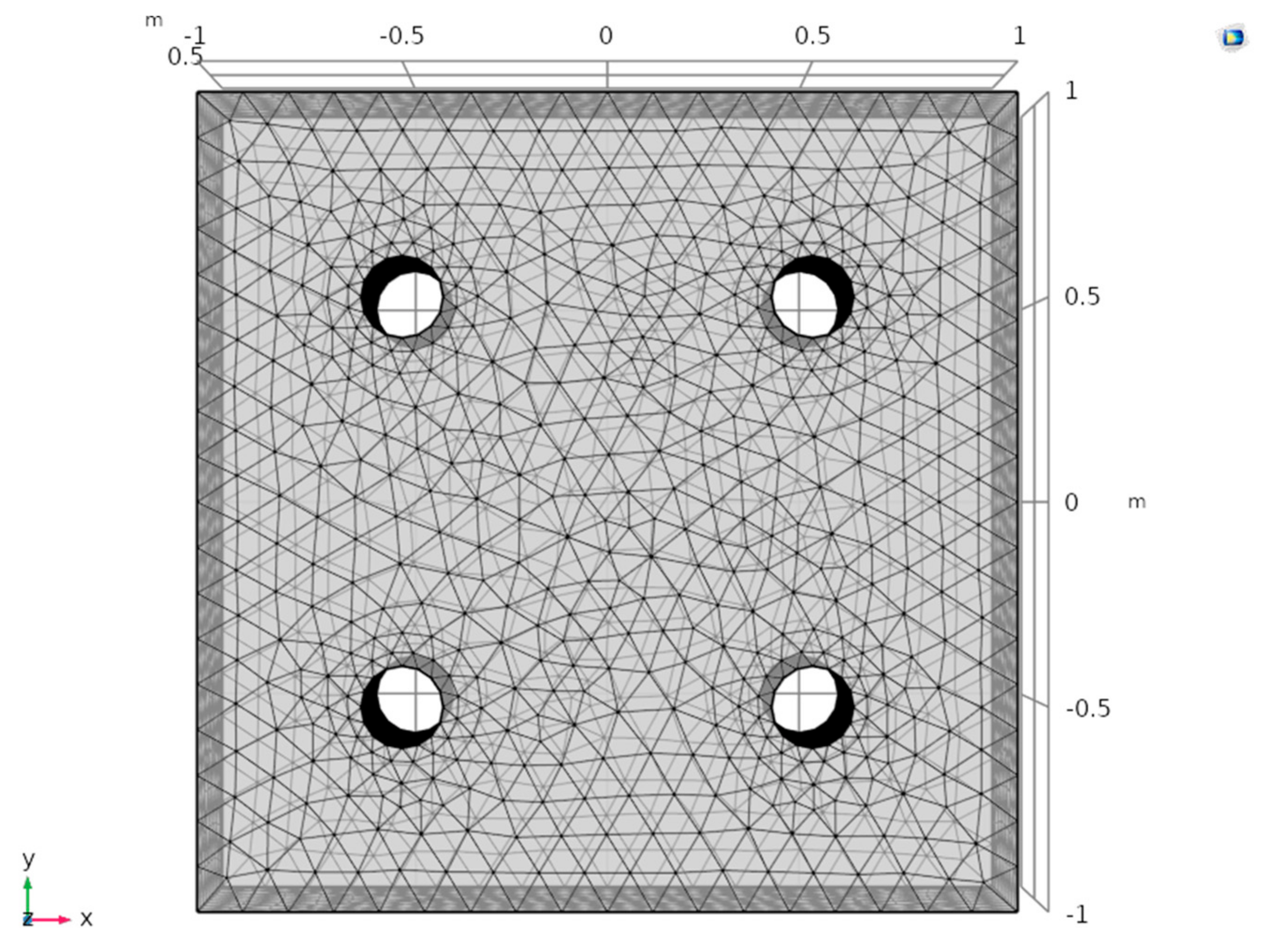
As shown in Figure 2, the model is divided into a group of unstructured tetrahedrons with a maximum cell size of 0.11 m, a minimum cell size of 0.008 m, a maximum growth rate of adjacent elements of 1.4, and a ratio of boundary cell size to radius of curvature of 0.4. The mesh is automatically generated by COMSOL according to the corresponding parameters.
2.1.2. Theoretical Derivation
Transient thermodynamic modeling was carried out and the corresponding ordinary differential control equation is:
where: T (SI unit: k) is the temperature; t (SI unit: s) is the time; ρ (SI unit: kg/m3) is the soil density; cp (SI unit: J/(kg K)) is the constant pressure heat capacity; cp,pi (SI unit: J/(kg K)) is the specific heat capacity of the medium under pressure pi; keff, kpi and k are effective thermal conductivity, medium thermal conductivity and pollutant thermal conductivity, respectively; θpi is the volume fraction of solid material, and u (SI unit: M/s) is the velocity field of fluid in the model, which can be in the form of analytical expression or the velocity field of fluid flow interface; Q is heat sources of the system.
The first term on the left of Equation (1) represents the change of temperature with time, and its coefficient is given by Equation (3), which is the effective volume heat capacity considering the properties of solid and fluid. The second term is the convection term, which is the change of heat under the action of reaction velocity field. The third term is the heat conduction term, which represents the heat change in heat conduction. Equation (2) is Fourier’s law of thermal conductivity, that is, the change of heat under the action of effective thermal conductivity. Equation (4) is the calculation formula of effective thermal conductivity, which characterizes the relationship between effective thermal conductivity and the volume fraction of solid material.
2.1.3. Simulation Conditions and Basic Assumptions
Related assumptions are as follows. (1) Assume that the soil is a uniform porous medium and ignore the thermal conductivity of other phase components. (2) The porous medium is in local thermal equilibrium and the effective thermal conductivity satisfies the volume average. The effective thermal conductivity is the same in all directions. (3) The heat source is an ideal heat source, the temperature is the same everywhere on the heat source surface, and there is no contact resistance and no heat transfer loss. (4) The heat diffusion from the soil to the surface air above the soil and the power loss during heating are ignored. (5) Except for the heating shaft wall, other vertical surfaces are thermally insulated.
The corresponding initial simulation conditions are as follows. The initial soil temperature is 273.15 K, and the four heating well walls are distributed with a heat source of 2000 W/m2. The simulation step size is 10 min, and the simulation time is 900 min. In the simulation, the relative tolerance is set to 0.01 and the tolerance factor set to 0.1. The absolute tolerance is the product of the relative tolerance and the tolerance factor, and also applies to scaled variables.
The simulation step size and mesh generation meet the accuracy requirements of repairing polluted soil with SVE technology in industry. The radius of influence (ROI) of the SVE system is usually more than 1 m, and the minimum heating well spacing used in the experiment is 1, which is within the ROI.
The thermodynamic parameters of porous media and pollutants are shown in Table 1:
2.2. Darcy’s Law
2.2.1. Model Establishment
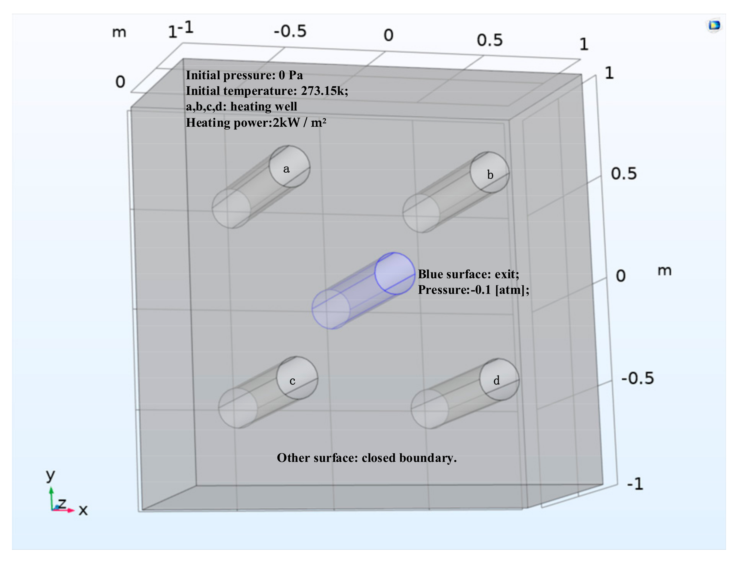
On the basis of the original model, an air extraction port with a diameter of 1 dm is added in the middle of the square surface. The whole model is shown in Figure 3:
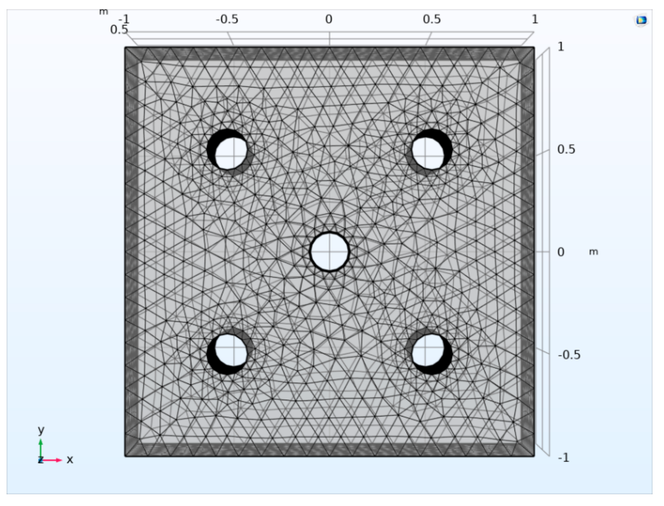
The grid division is still controlled by the physical field. The result of grid division is shown in Figure 4.
2.2.2. Theoretical Basis
Darcy’s law was developed by French engineer Darcy through experiments. It describes the linear relationship between fluid seepage velocity and hydraulic gradient in saturated sand:
where Qf is the total flow, k is the inherent permeability of the medium, A is the cross-sectional area of the medium, (Pb − Pa) is the total pressure drop, L is the distance of pressure drop, and µ is the viscosity of the fluid. The formula indicates that the seepage flow Qf is directly proportional to the upstream and downstream water pressure drop (Pb − Pa) and the cross-sectional area A perpendicular to the flow direction, but inversely proportional to the seepage length L.
Because the porous medium used in the experimental model is soil, not idealized sand, the effects of viscosity and various internal and external pressures should be calculated. Moreover, due to the existence of an air extraction port, complex force field changes occur in the soil in the process of air extraction, such as the effect of various resistances. Because simulating the flow of porous media at the micro level requires a lot of computational resources and time, the detailed structure of porous media is ignored here. Instead, two macro quantities of porosity and permeability are used to describe the properties of porous media at the macro level, which greatly reduce the computational cost. The corresponding governing equation is:
where εp represents the porosity of the soil, ρ represents the density of soil, u represents the flow velocity field of medium, Qm represents heat source, κ represents the permeability of the soil, μ is the dynamic viscosity of the soil and P is the fluid pressure. The first equation represents the relationship between soil porosity and heat source distribution, and the second equation represents the relationship between fluid velocity field and soil permeability and pressure drop. The simulation parameters of this experiment are still set according to Table 1.
2.2.3. Basic Assumptions and Simulation Conditions
To add Darcy’s law physical field to the COMSOL simulation model, the following assumptions need to be made for the whole model: (1) the soil medium is homogeneous and the relevant parameters are isotropic; (2) the pores of porous media are uniformly filled with pollutants; (3) the pressure difference of each part of the extraction hole wall is evenly distributed; (4) there is no displacement at each point at the boundary; (5) the effect of gravity on the pressure distribution is ignored.
We used the equation in our previous article [24] to calculate the Reynolds number of the flowing fluid to ensure that the fluid is laminar, so its motion can be described by Darcy’s law.
In the corresponding initial simulation conditions the extraction hole wall pressure is 0.1 [atm] lower than the average pressure inside the soil. Except for the extraction hole wall, there is no gas exchange at other boundaries. The remaining conditions for the coupled field simulation are the same as for the porous media temperature simulation.
During the simulation, the properties of each material are as shown in Table 1.
2.3. Energy Efficiency
Since the boiling point of ethylbenzene is 409.35 K and the critical temperature is 616.25 K, 620 K is taken as the effective removal temperature of ethylbenzene. The area with a temperature of 620 K and above can be regarded as the effective heating area. The optimal heating time interval can be obtained by calculating the relationship between the effective heating area and time. Because the heat source is a generalized source and the model boundary is closed, the total energy input power of the system is constant, and the change relationship between the effective heating area and time is the energy consumption efficiency of the whole system with heating.
3. Results
3.1. Numerical Simulation of Temperature Field Changes in Heat Transfer Process of Porous Media
According to the given initial simulation conditions, a transient study was adopted, the time step was 10 min, and the simulation time range was 0–15 h. The temperature field distribution of porous medium heat transfer model in the range of 0–15 h in the process of SVE was simulated. Some results are shown in the figure below. Since the temperature at all positions of the model was 293.15 K at the initial time, the temperature field distribution at the initial time was ignored.
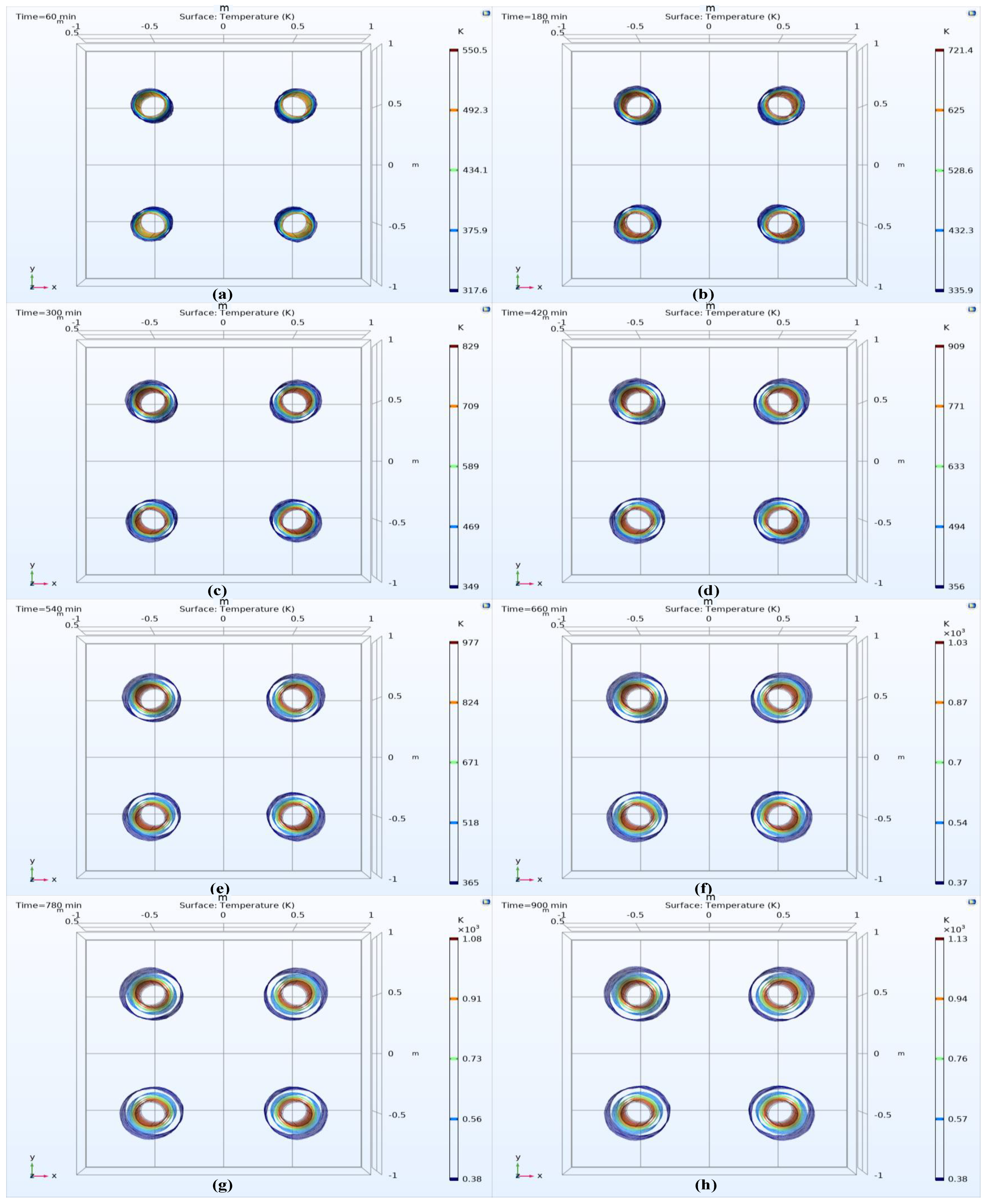
It can be seen from Figure 5 that after heating, the heat begins to transfer from the heat source to the surrounding, and the position of the aperture in the corresponding figure gradually increases. However, according to Fourier’s law, the efficiency of heat conduction is directly proportional to the temperature gradient, that is, the widening speed of the outer ring of the aperture gradually decreases with time, which is reflected in the figure. After 9 h, the change of the position of the outer ring of the aperture is less obvious. This shows that with heating, the whole temperature field distribution tends to be stable, the increment of effective heating area gradually decreases, and the overall energy consumption efficiency of SVE system gradually decreases. In order to see this characteristic, a temperature isosurface distribution was drawn, as shown in Figure 6.
It can be seen from Figure 6 that the central temperature of the heat source rises rapidly at the beginning of heating, and then the increase of the central temperature of the heat source decreases gradually every hour, and the central temperature of the heat source rises steadily after the fifth hour. In the 10th to 15th hour, the temperature of the outermost ring of the medium value surface is the same, the widening speed of the outer ring of the whole figure is slow, and the whole temperature field distribution tends to be stable, indicating that the increment of the effective heating area decreases gradually. This is the same as the conclusion obtained from the previous analysis of the temperature field distribution diagram.
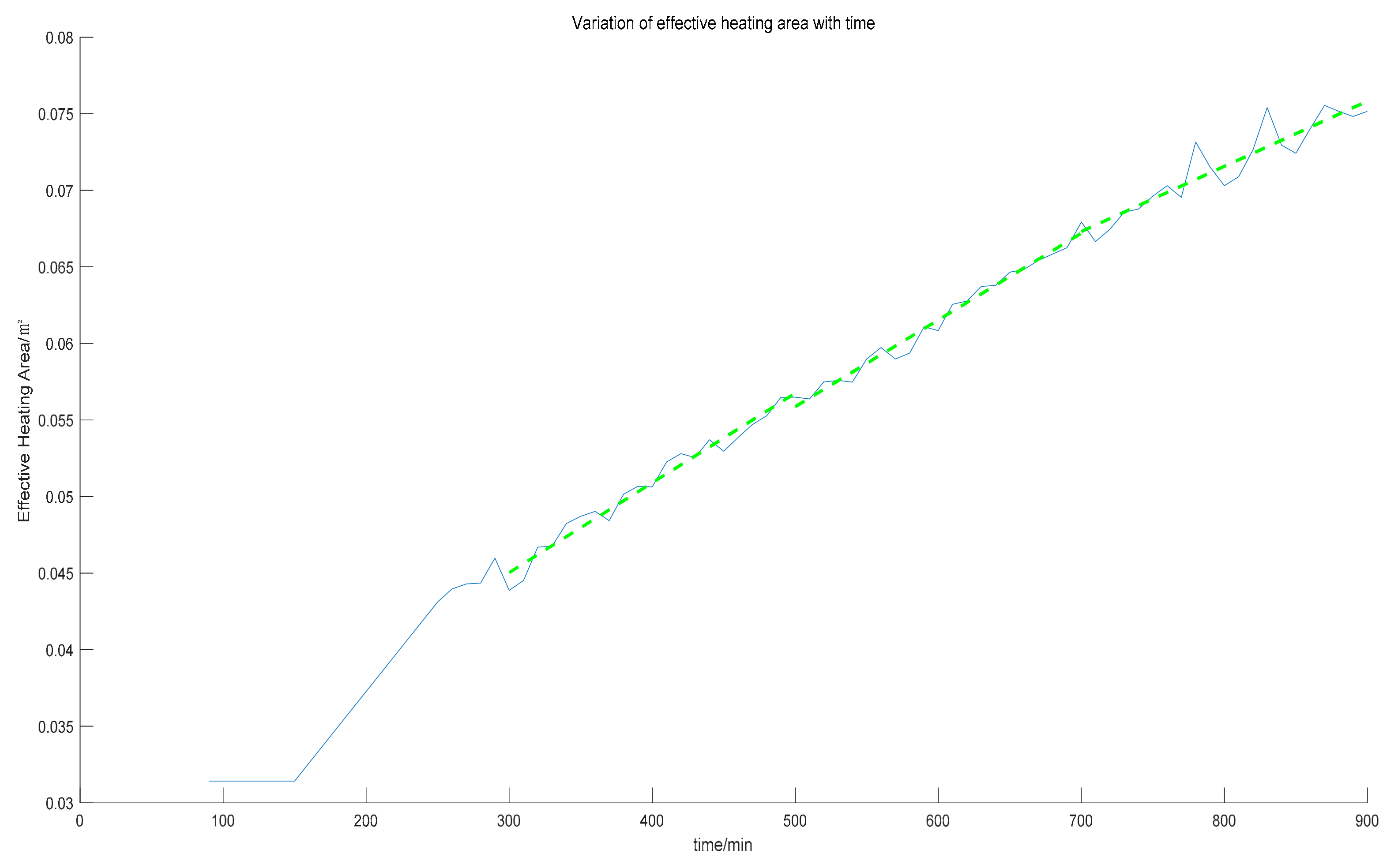
Since the temperature distribution along the vertical direction of the whole model is almost the same, as defined in Section 2.1, the effective heating area can be simplified as the soil area enveloped by the curve of temperature 620 K on the horizontal plane, rather than the volume of soil column. It can be seen from the figure that the effective heating area gradually expands with time. There is an obvious band break after the start time in the figure, because the temperature changes greatly at the beginning of heating, so there is no point with a temperature of about 620 K in this time period. With the increase of heating time, the temperature fluctuation of each point at the boundary of the effective heating area gradually decreases, so more and more points with a temperature of about 620 K are detected.
The effective heating area on the xoy plane was calculated, and its variation with time is shown in Figure 7.
The slope of the curve begins to decrease gradually at the 600th minute, the increment of the effective heating area becomes smaller, and the energy consumption efficiency of the system decreases. The conclusion is the same as that of the numerical simulation.
3.2. Numerical Simulation of Temperature Field Changes under Pollutant Migration
The physical field of Darcy’s law was introduced to simulate the coupling of heat transfer field of porous media and Darcy’s velocity field. The pressure at the extraction port was set to −10132.5 Pa, which is within an easily accessible and relatively safe pressure range. Since the extraction port takes away part of the heat energy, the simulation time was set to 1800 min.
The velocity field distribution of coupling simulation is shown in Figure 8.
The variation relationship of soil temperature field with time under the action of Darcy’s law physical field is shown in Figure 9.
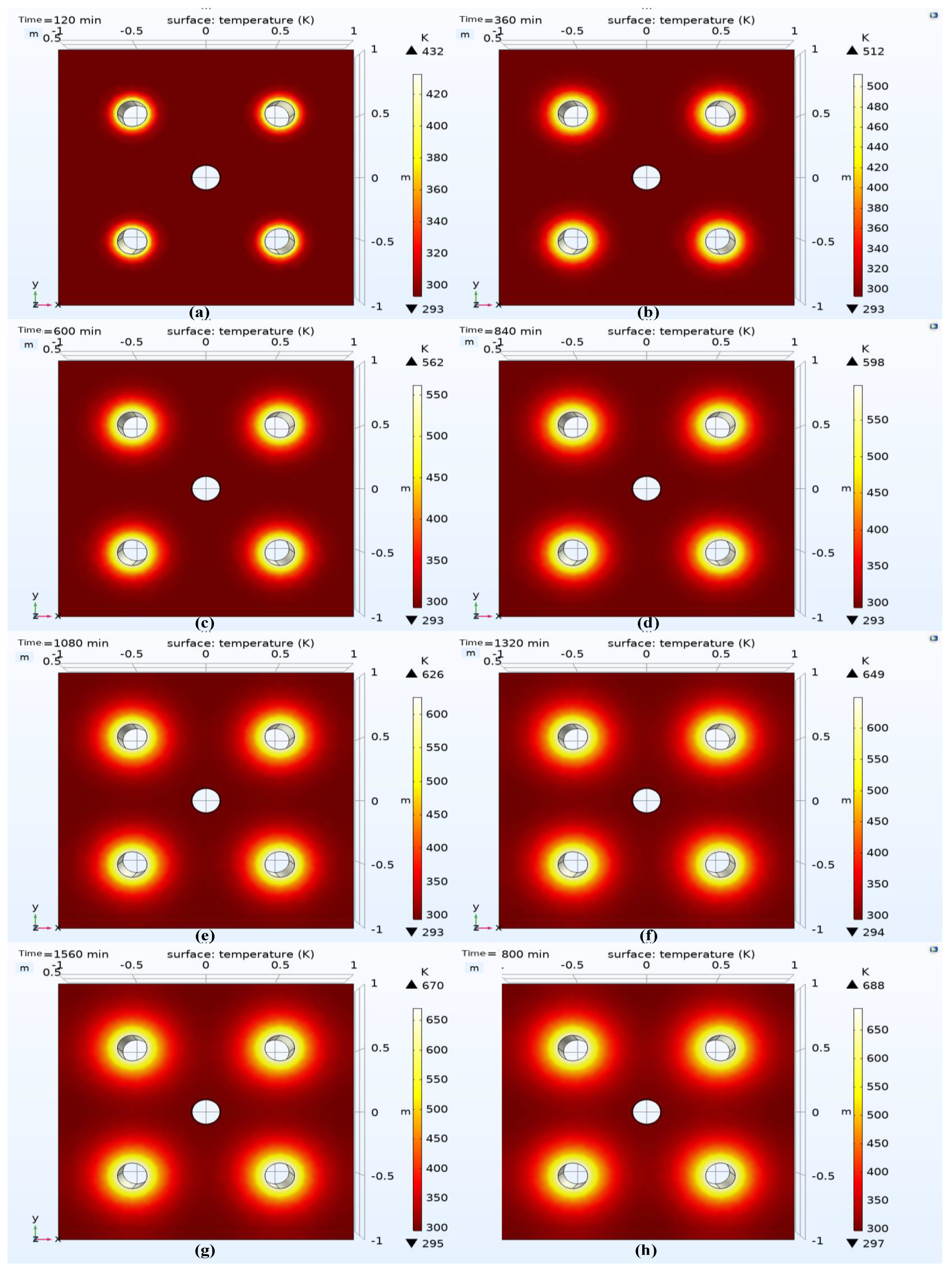
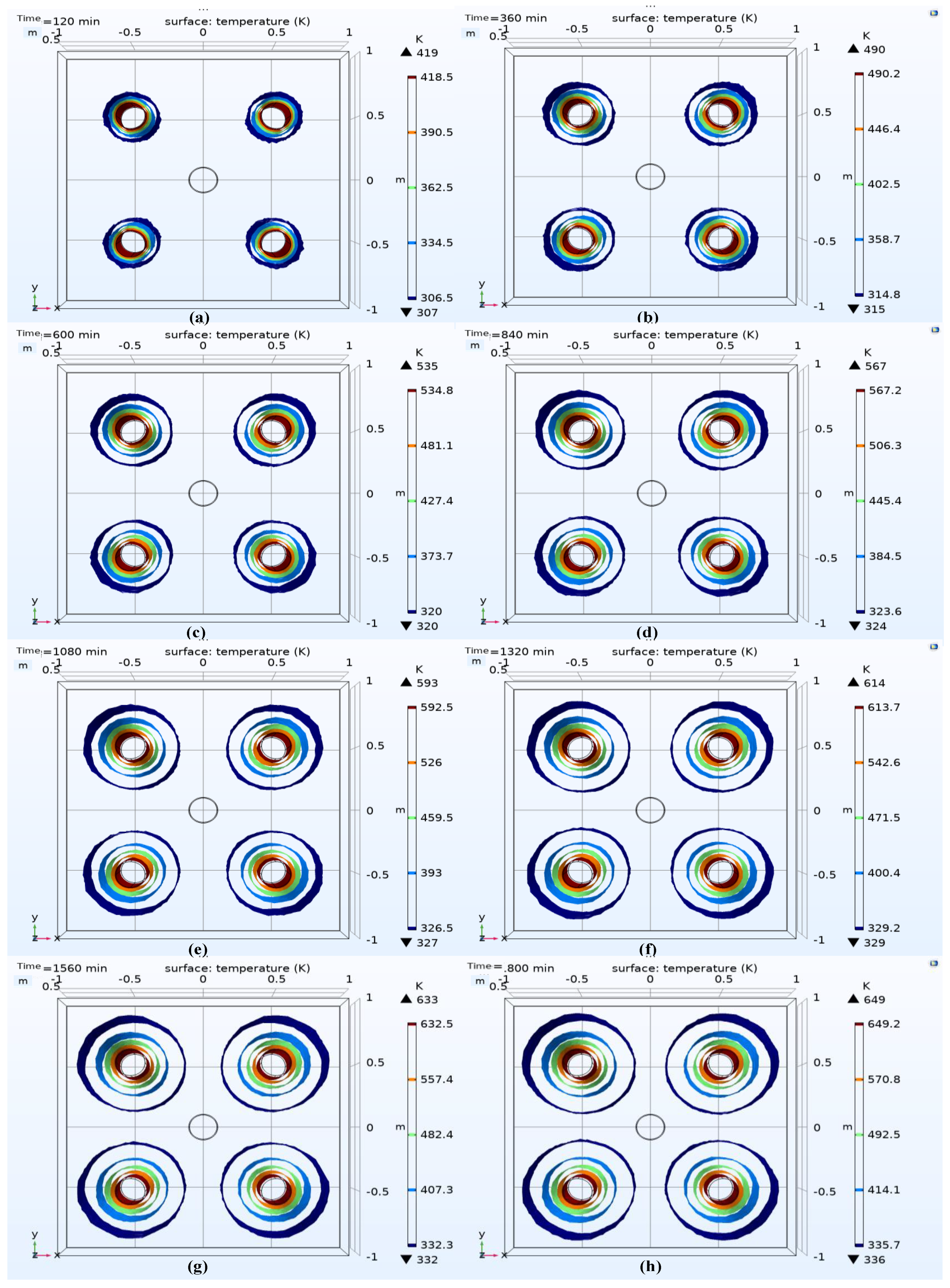
Comparing images of the same simulation time in Figure 6 and Figure 9, such as the temperature field distribution in 840th minute, it can be seen that the distance between the two different temperature isosurfaces is almost the same. However, the temperature gradient of the different temperature isosurfaces in Figure 6 is about three times that of the corresponding temperature gradient in Figure 9, indicating that the temperature field distribution in Figure 9 is more uniform. This shows that the Darcy field improves the utilization efficiency of the SVE model for the heat source, and we believe that pollutants can be effectively removed when the temperature is higher than 620 K. However, at the same time, due to decrease of the maximum temperature, some of the original effective heating areas cannot reach the effective heating temperature within the same heating time. Therefore, it is necessary to increase the heat source power or prolong the heating time. In order to more intuitively reflect the change of temperature field distribution, a temperature isosurface of the coupling field was made, as showed in Figure 10.
4. Discussion and Conclusions
The heat transfer simulation of porous media shows that when the soil is heated by a heat source with constant thermal power, the soil heat is rapidly transferred from the heat source to the surroundings, and the effective heating area gradually increases. With the heating time getting longer, the added value of the effective heating area of the soil gradually decreases, and the energy consumption efficiency of the system decreases.
By adding the Darcy field simulation, it was found that after adding the Darcy velocity field outlet, the temperature of the heat source decreases significantly and the heat diffusion area increases significantly. The utilization efficiency of the heat source is significantly improved because, we believe, that when the temperature is higher than 620 K, the pollutants can be effectively removed and temperature has little effect on the pollutant removal efficiency. However, due to the decrease of the heat source temperature, the temperature rise rate in the original heating area is lower than that without Darcy field. To continue to meet a certain effective heating area, the heating time can be extended, or the heat source power can be increased.
Through simulation, we obtained the soil temperature field distribution for the first 1800 min under the specific heating well distribution, and through the analysis of these data we verified that the extraction well could improve the utilization efficiency of the heat source of the SVE system.
However, the transformation between the phases of NAPL was not involved in this model, and the changes in the characteristics of porous media caused by the removal of ethylbenzene were not considered. We think that the ethylbenzene can be successfully removed in the region reaching this temperature. In fact, since the thermal conductivity of air is lower than that of ethylbenzene, the actual temperature of the peripheral area is lower than the simulated temperature, which means that a longer heating time is required to achieve the same removal effect.
In future research we will continue to improve our model, define NAPL materials, add a transformation simulation between different phases of NAPL, and optimize the distribution of the heating wells.
Author Contributions
Conceptualization, S.X.; formal analysis, S.R.; funding acquisition, N.W.; methodology, S.X.; project administration, Y.S.; software, S.R.; supervision, Y.W.; validation, S.R.; writing—original draft, S.R.; writing—review & editing, Y.W. All authors will be informed about each step of manuscript processing including submission, revision, revision reminder, etc. via emails from our system or the assigned Assistant Editor. All authors have read and agreed to the published version of the manuscript.
Funding
This research was funded by [Youth Fund of National Natural Science Foundation of China] grant number 52105044.
Institutional Review Board Statement
Not applicable.
Informed Consent Statement
Not applicable.
Data Availability Statement
The data provided in this study can be provided at the request of the corresponding author. Since [The data in this article will be used to develop equipment in cooperation with Center International Group], these data cannot be made public.
Conflicts of Interest
The authors declare no conflict of interest.
References
- Todd, H.; Valina, S.; Tom, S.; Lyverse, M. Mechanism for detecting NAPL using electrical resistivity imaging. J. Contam. Hydrol. 2017, 205, 57–69. [Google Scholar]
- Gabriele De, S.; Carlo, L.; Francesca, P.; Galli, G.; Tuccimei, P.; Curatolo, P.; Giorgi, R. Soil radon survey to assess NAPL contamination from an ancient spill. Do kerosene vapors affect radon partition? J. Environ. Radioact. 2017, 171, 138–147. [Google Scholar]
- Motasem YD, A.; Su, K.N.; Mustafa, M.B.; Kamaruddin, S.A.; Ishak, W.M.F. Influence of macro-pores on DNAPL migration in double-porosity soil using light transmission visualization method. Transp. Porous Media 2017, 117, 103–123. [Google Scholar]
- Tannaz, P.; Nathaly, L.A.; Raaid, A. Application of nanotechnology in removal of NAPLs from contaminated aquifers, A source clean-up experimental study. Clean Technol. Environ. Policy 2018, 20, 427–433. [Google Scholar]
- Ramezanzadeh, M.; Aminnaji, M.; Rezanezhad, F.; Ghazanfari, M.H.; Babaei, M. Dissolution and remobilization of NAPL in surfactant-enhanced aquifer remediation from microscopic scale simulations. Chemosphere 2022, 289, 133177. [Google Scholar] [CrossRef]
- Javanbakht, G.; Arshadi, M.; Qin, T.; Goual, L. Micro-scale displacement of NAPL by surfactant and microemulsion in heterogeneous porous media. Adv. Water Resour. 2017, 105, 173–187. [Google Scholar] [CrossRef]
- Huo, L.; Liu, G.; Yang, X.; Ahmad, Z.; Zhong, H. Surfactant-enhanced aquifer remediation, Mechanisms, influences, limitations and the countermeasures. Chemosphere 2020, 252, 126620. [Google Scholar] [CrossRef]
- Sabooniha, E.; Rokhforouz, M.-R.; Kazemi, A.; Ayatollahi, S. Numerical analysis of two-phase flow in heterogeneous porous media during pre-flush stage of matrix acidizing, Optimization by response surface methodology. Phys. Fluids 2021, 33, 53605. [Google Scholar] [CrossRef]
- Koproch, N.; Dahmke, A.; Köber, R. The aqueous solubility of common organic groundwater contaminants as a function of temperature between 5 and 70 °C. Chemosphere 2019, 217, 166–175. [Google Scholar] [CrossRef]
- Ni, Z.; van Gaans, P.; Smit, M.; Rijnaarts, H.; Grotenhuis, T. Combination of aquifer thermal energy storage and enhanced bioremediation, Resilience of reductive dechlorination to redox changes. Appl. Microbiol. Biotechnol. 2016, 100, 3767–3780. [Google Scholar] [CrossRef]
- Beyer, C.; Popp, S.; Bauser, S. Simulation of temperature effects on groundwater flow, contaminant dissolution, transport and biodegradation due to shallow geothermal use. Environ. Earth Sci. 2016, 55, 1244. [Google Scholar] [CrossRef]
- Ni, Z.; van Gaans, P.; Smit, M.; Rijnaarts, H. Grotenhuis, Biodegradation of cis-1,2-Dichloroethene in simulated underground thermal energy storage systems. Environ. Sci. Technol. 2015, 49, 13519–13527. [Google Scholar] [CrossRef]
- Huang, J.; Goltz, M.N. Analytical solutions for a soil vapor extraction model that incorporates gas phase dispersion and molecular diffusion. J. Hydrol. 2017, 549, 452–460. [Google Scholar] [CrossRef]
- Esrael, D.; Kacem, M.; Benadda, B. Modelling mass transfer during venting/soil vapour extraction, Non-aqueous phase liquid/gas mass transfer coefficient estimation. J. Contam. Hydrol. 2017, 202, 70–79. [Google Scholar] [CrossRef]
- Yu, Y.; Liu, L.; Yang, C.; Kang, W.; Yan, Z.; Zhu, Y.; Wang, J.; Zhang, H. Removal kinetics of petroleum hydrocarbons from low-permeable soil by sand mixing and thermal enhancement of soil vapor extraction. Chemosphere 2019, 236, 124319. [Google Scholar] [CrossRef]
- Liang, C.; Yang, S. Foam flushing with soil vapor extraction for enhanced treatment of diesel contaminated soils in a one-dimensional column. Chemosphere 2021, 285, 131471. [Google Scholar] [CrossRef]
- Yang, Y.; Li, J.; Xi, B.; Wang, Y.; Tang, J.; Wang, Y.; Zhao, C. Modeling BTEX migration with soil vapor extraction remediation under low-temperature conditions. J. Environ. Manag. 2017, 203, 114–122. [Google Scholar] [CrossRef]
- Albergaria, J.T.; Alvim-Ferraz, M.d.M.; Delerue-Matos, C. Soil vapor extraction in sandy soils, Influence of airflow rate. Chemosphere 2008, 73, 1557–1561. [Google Scholar] [CrossRef] [Green Version]
- You, K.; Zhan, H. Can atmospheric pressure and water table fluctuations be neglected in soil vapor extraction? Adv. Water Resour. 2012, 35, 41–54. [Google Scholar] [CrossRef]
- Shi, J.; Yang, Y.; Lu, H.; Xi, B.; Li, J.; Xiao, C.; Wang, Y.; Tang, J. Effect of water-level fluctuation on the removal of benzene from soil by SVE. Chemosphere 2021, 274, 129796. [Google Scholar] [CrossRef]
- Albergaria, J.T.; Alvim-Ferraz, M.d.M.; Delerue-Matos, C. Remediation efficiency of vapour extraction of sandy soils contaminated with cyclohexane, Influence of air flow rate, water and natural organic matter content. Environ. Pollut. 2006, 143, 146–152. [Google Scholar] [CrossRef] [Green Version]
- Soares, A.A.; Albergaria, J.T.; Domingues, V.F.; Alvim-Ferraz, M.d.M.; Delerue-Matos, C. Remediation of soils combining soil vapor extraction and bioremediation, Benzene. Chemosphere 2010, 80, 823–828. [Google Scholar] [CrossRef] [Green Version]
- Kempa, T.; Marschalko, M.; Yilmaz, I.; Lacková, E.; Kubečka, K.; Stalmachová, B.; Bouchal, T.; Bednárik, M.; Drusa, M.; Bendová, M. In-situ remediation of the contaminated soils in Ostrava city (Czech Republic) by steam curing/vapor. Eng. Geol. 2013, 154, 42–55. [Google Scholar] [CrossRef]
- Wang, N.; Liu, Q.; Shi, Y.; Wang, S.; Zhang, X.; Han, C.; Wang, Y.; Cai, M.; Ji, X. Modeling and Simulation of an Invasive Mild Hypothermic Blood Cooling System. Chin. J. Mech. Eng. 2021, 34, 23. [Google Scholar] [CrossRef]
Figure 1.
Heat transfer model of porous media. There is no fluid flow and heat exchange on the closed boundary. Considering that many cells are closely distributed in the heating site, the four planes on the outside parallel to the axis of the heating well are periodic boundaries.
Figure 1.
Heat transfer model of porous media. There is no fluid flow and heat exchange on the closed boundary. Considering that many cells are closely distributed in the heating site, the four planes on the outside parallel to the axis of the heating well are periodic boundaries.

Figure 2.
Grid division of the porous medium heat transfer model.

Figure 3.
Simulation model of Darcy’s law. As showed in the figure, it is still assumed that the upper boundary of the model is the ground, the main material medium is soil, and the fluid medium in the porous medium is ethylbenzene(liquid). The properties are shown in Table 1. There is no fluid flow and heat exchange on the closed boundary. The four planes on the outside parallel to the axis of the heating well are periodic boundaries.

Figure 4.
Grid division of Darcy’s law simulation model.

Figure 5.
Temperature field distribution in the porous media model in 1~15 h. Subfigures (a–h) show the temperature field distribution of porous media every two hours after the first hour of simulation. The temperatures represented by different colors are given in the legend.
Figure 5.
Temperature field distribution in the porous media model in 1~15 h. Subfigures (a–h) show the temperature field distribution of porous media every two hours after the first hour of simulation. The temperatures represented by different colors are given in the legend.

Figure 6.
Temperature isosurface in porous medium model in 1~15 h. Subfigures (a–h) show the temperature isosurface of porous media every two hours after the first hour of simulation. The temperatures of different surfaces are given in the legend.
Figure 6.
Temperature isosurface in porous medium model in 1~15 h. Subfigures (a–h) show the temperature isosurface of porous media every two hours after the first hour of simulation. The temperatures of different surfaces are given in the legend.

Figure 7.
Variation curve of effective heating area versus time. Due to the problem of boundary accuracy, there are many fluctuations in the curve. The dotted line in the figure is the linear regression curve corresponding to interval data.
Figure 7.
Variation curve of effective heating area versus time. Due to the problem of boundary accuracy, there are many fluctuations in the curve. The dotted line in the figure is the linear regression curve corresponding to interval data.

Figure 8.
Distribution of velocity field versus time for coupled simulation. Subfigures (a–h) use streamline to represent the fluid velocity distribution in porous media every 4 h after the second hour of simulation. The speed value is given by the legend, and the speed direction is the same as the arrow direction.

Figure 9.
Variation of soil temperature with time under the coupling of heat transfer in porous media and Darcy velocity field. Subfigures (a–h) show the temperature field distribution of porous media every 4 h after the second hour of simulation. The temperature corresponding to different colors is given in the legend.

Figure 10.
Isosurface of soil temperature distribution in the coupling field. Subgraphs (a–h) show the temperature isosurface of porous media every 4 h after the second hour of simulation. The temperatures of different surfaces are given in the legend.
Figure 10.
Isosurface of soil temperature distribution in the coupling field. Subgraphs (a–h) show the temperature isosurface of porous media every 4 h after the second hour of simulation. The temperatures of different surfaces are given in the legend.


Table 1.
Heat transfer simulation parameters of porous media.
| Material | Thermal Conductivity k/[W/(m·K)] | Constant Pressure Heat Capacity Cp/[J/(kg·K)] | Density ρ/[kg/m3] | Volume Fraction θpi | Porosity ε | Permeability κ/m2 | Dynamic Viscosity μ/[Pa·s] |
|---|---|---|---|---|---|---|---|
| Porous Medium | 0.70 | 1010 | 2300 | 0.82 | 0.3 | 0.00179 | |
| Contam-inants | 0.129 | 1697 | 870 | - | - | - | 6.1 × 10⁻⁴ |
Publisher’s Note: MDPI stays neutral with regard to jurisdictional claims in published maps and institutional affiliations. |
© 2022 by the authors. Licensee MDPI, Basel, Switzerland. This article is an open access article distributed under the terms and conditions of the Creative Commons Attribution (CC BY) license (https://creativecommons.org/licenses/by/4.0/).
Share and Cite
MDPI and ACS Style
Shi, Y.; Rui, S.; Xu, S.; Wang, N.; Wang, Y. COMSOL Modeling of Heat Transfer in SVE Process. Environments 2022, 9, 58. https://0-doi-org.brum.beds.ac.uk/10.3390/environments9050058
AMA Style
Shi Y, Rui S, Xu S, Wang N, Wang Y. COMSOL Modeling of Heat Transfer in SVE Process. Environments. 2022; 9(5):58. https://0-doi-org.brum.beds.ac.uk/10.3390/environments9050058
Chicago/Turabian StyleShi, Yan, Shuwang Rui, Shaofeng Xu, Na Wang, and Yixuan Wang. 2022. "COMSOL Modeling of Heat Transfer in SVE Process" Environments 9, no. 5: 58. https://0-doi-org.brum.beds.ac.uk/10.3390/environments9050058
Note that from the first issue of 2016, this journal uses article numbers instead of page numbers. See further details here.