1. Introduction
Fuzzy logic has proven to be a particularly useful tool in the hands of engineers, and its use in recent decades has been widespread in hydrology and hydraulics. Fuzzy linear regression provides a functional fuzzy relationship between dependent and independent variables, where uncertainty manifests itself in the coefficients of the independent variables.
Next, the fuzzy linear regression of Tanaka [
1] is used. In general, the fuzzy regression analysis gives a fuzzy functional relationship between the dependent and independent variables [
2,
3]. In contrast to the statistical regression, the fuzzy regression model of Tanaka [
1] has no error term, while the uncertainty is incorporated into the model with the use of fuzzy numbers [
4,
5]. The data of the fuzzy regression can be either fuzzy or crisp. Usually, the data are rather crisp numbers (observed data), and thus, the uncertainty arises from the used fuzzy model, that is, the fuzzy coefficients. The inclusion property of the produced fuzzy band, that is, the requirement that all the data must be included within the produced fuzzy band, creates the constraints.
Papadopoulos et al. and Spiliotis et al. [
5,
6] proposed a fuzzy hybrid frequency factor-based method, with the use of fuzzy regression, in order to improve the couple between the theoretical and the observed probability distributions. These articles deal with either annual cumulative streamflow or precipitation. In this work, the annual maximum flow is studied, and furthermore, the fuzzified likelihood is used as an additional measure of suitability.
2. Basic Notations and the Proposed Methodology
2.1. Fundamentals of Fuzzy Sets and Logic
A fuzzy set A on a universe set X is a mapping , assigning to each element a degree of membership . The membership function A(x) can be also presented as .
If
A is a fuzzy set, and let any number
by the α-cut,
and the strong α-cut,
,the crisp sets
are defined, respectively as:
The 0-cut can be defined as follows:
In order to have a closed interval containing the boundaries, Hanss [
7] proposed the phrase worst-case interval
W, which is the union of the 0-strongcut and the boundaries. It is worth noting that, by using the α-cut concept, we can move from the fuzzy sets to the conventional crisp mathematical methodologies.
A special kind of fuzzy sets is the fuzzy numbers. In this work, fuzzy symmetric triangular numbers are used, which are special kinds of fuzzy numbers. The fuzzy symmetric triangular numbers have the following membership function:
in which a is the center and
w the spread of the fuzzy number.
The operation of the usual crisp functions, if the inputs are fuzzy sets, can be extended based on the extension principle. In most cases, it is preferable to use a-cuts in the fuzzy analysis [
8]. If
g is a continuous function in the extension principle, the use of a-cuts can be made by determining the a-cuts of the function
f, as follows [
9,
10]. Then, based on the min intersection, it holds:
From the theorem of global existence for maxima and minima of functions with many variables, it is known that, if the domain of a real function is closed and bounded and the real function is continuous, then the function will have its absolute minimum and maximum values at some points in the domain [
8,
11]. Based on this theorem, it is evident that the α-cut for any real continuous function with real variables in this domain can be determined, given that the inputs are fuzzy triangular numbers [
8].
2.2. Fuzzy Linear Regression
The fuzzy linear regression model proposed by Tanaka [
1] has the following form:
where
n is the number of independent variables
xij (here only
n =1 which is related with the observed return period),
M is the number of data,
is the fuzzy predicted value of the dependent variable considering the
jth data (here, the maximum annual flow).
According to Tanaka [
1], all the data must be included within the produced fuzzy band (inclusion principle). Based on the extension principle and the concept of α-cuts, the inclusion principle is equivalent to (by using fuzzy symmetrical triangular numbers as coefficients):
where
ai is the center and
ci the spread of the fuzzy number which represents the fuzzy coefficient.
Finally, the sum of the produced semi-widths for the produced dependent variable for all the data is proposed as an objective function:
In other words, the problem of fuzzy linear regression is reduced to a linear programming problem [
1,
4].
2.3. Observed Probabilities
Let a historical sample. The rank order method involves ordering the data from the largest hydrological value to the smallest hydrological value, assigning a rank of 1 to the largest value and a rank of
N to the smallest value. An empirical distribution is used to compute the plotting position probabilities as follows [
12]:
Therefore, the cumulative probability or non-exceedance probability can be determined as follows:
The concept of the observed probability is critical, since the suitability of the used theoretical probability function is based on the comparison between the observed and the theoretical probability values.
2.4. Generalized Extreme Value (GEV) Distribution
The probability density function of the GEV distribution is of the form [
13]:
The GEV distribution function is as follows [
14]:
The distribution function of
x given by Equation (12) can be written in the inverse form [
13]:
By substituting
where
T
is the return period, the T-year quantile estimate of the annual maximum flow,
, is obtained
as follows:
Csis the skewness coefficient, which can be estimated as:
Furthermore,
a’ is the asymmetry of a sample, of which the unbiased estimation is:
where
N is the magnitude of the historical sample. Approximate relationships between the value of
k and the skewness coefficient
CS, obtained through regression analysis, are given in pages 225, 226 and 227 (7.1.12, 7.1.13 and 7.1.14) in [
13]. This approach was adopted by the authors.
In this article, the term
is considered as a crisp number, while the terms
and
are considered as fuzzy numbers. Therefore, the following fuzzy regression model is modulated:
in which , , are the fuzzified dependent variable, the constant term and the coefficient of the considered independent variable. It should be clarified that the independent variables, as well as all the observed values, are crisp numbers. The method does not require any transformation of the crisp data to fuzzy data.
2.5. The Extreme Value Type I EV1(2) Distribution
The probability density function of the EV1(2) distribution is given by the following equation [
13]:
The variable
x takes values in the range
. The distribution function of x is given by the following equation:
The EV1(2) distribution is a special case of the GEV distribution, discussed in
Section 2.4, in which the shape parameter
k is equal to zero. The distribution function of EV1(2) (Equation (14)) can be obtained in the inverse form as follows [
13]:
The T-year quantile is calculated by substituting
, where
T is the return period, to obtainthe following equation:
More specifically, the term
is considered as a crisp number, while the terms
and
are considered as fuzzy numbers. Inthe same way, by using the fuzzy linear regression, the following fuzzy relation is determined, with the aim of fuzzy linear regression model:
2.6. Measures of Suitability
Since a fuzzy approach is dealt, the usual statistical test cannot be used to check the suitability of the proposed model. The first model of suitability, which can be used, is the produced uncertainty of the produced fuzzy band,
J (Equation (8)):
where , , represent the number of data, the semi-width of the constant term and the semi- width of the independent variable coefficient, respectively.
In this article, the use of the likelihood is used as a measure of suitability (and not to determine the parameters). Since the parameters are fuzzy, then the fuzzified likelihood is constructed by determining the borders of the α-cut for the likelihood, for several representative values of the α-cut, as follows:
To summarize the proposed methodology, the following steps are adopted: (1) modulating the independent and dependent variables based on the Weibull 1939 empirical distribution and the examined theoretical probability distribution. (2) Applying fuzzy regression; (3) the magnitude of the produced fuzzy band and the fuzzfied likelihoods are used as suitability measures.
3. Case Study
The case under investigation is a northern region (Marino Pole) of the Strymonas River (
Figure 1). The Strymonas (Struma) River is one of the largest rivers in theBalkan Peninsula in terms of length, since it crosses the Bulgarian and Greek borders. It rises in the Vitosha Mountain in Bulgaria, and has its outlet in the Aegean Sea. Its drainage area is 17,330 km
2, of which 10,797 km
2 is in Bulgaria, 6295 km
2 is in Greece, and the rest is in North Macedonia. In Greece, it is the main waterway feeding and exiting from Lake Kerkini, a significant center for migratory wildfowl. The river’s length is 415 km (of which 290 km is in Bulgaria), making it the country’s fifth-longest and one of the longest rivers that run solely in the interior of the Balkans. Τhe location of the analysis is the Marino Pole, which is located in Bulgaria.
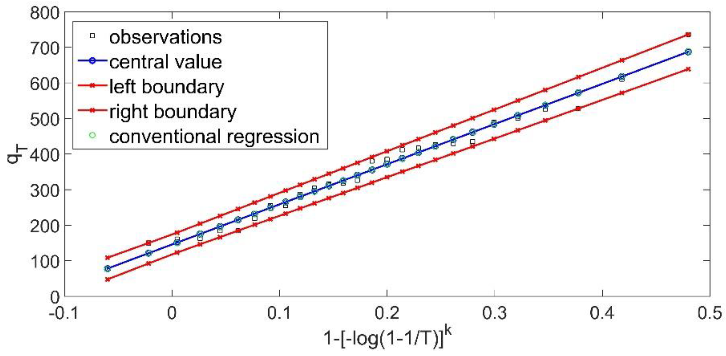
Firstly, the GEV theoretical probability distribution is examined. Since the fuzzy regression enables the determination of two parameters, the third parameter is estimated at the beginning of the method, based on the moment method. Hence, based on the sample, the skewness coefficient is
and finally,
. Subsequently, the fuzzy linear regression of Tanaka with the worst-case interval W is applied, which leads to the following fuzzy curve (
Figure 2):
Based on the solution, the sum of the produced semi-widths
(J) is:
Another interesting point of view is that, as can be seen from
Figure 2, all the (crisp)observations are included within the produced fuzzy band a property, which is not satisfied according to the conventional methodologies.
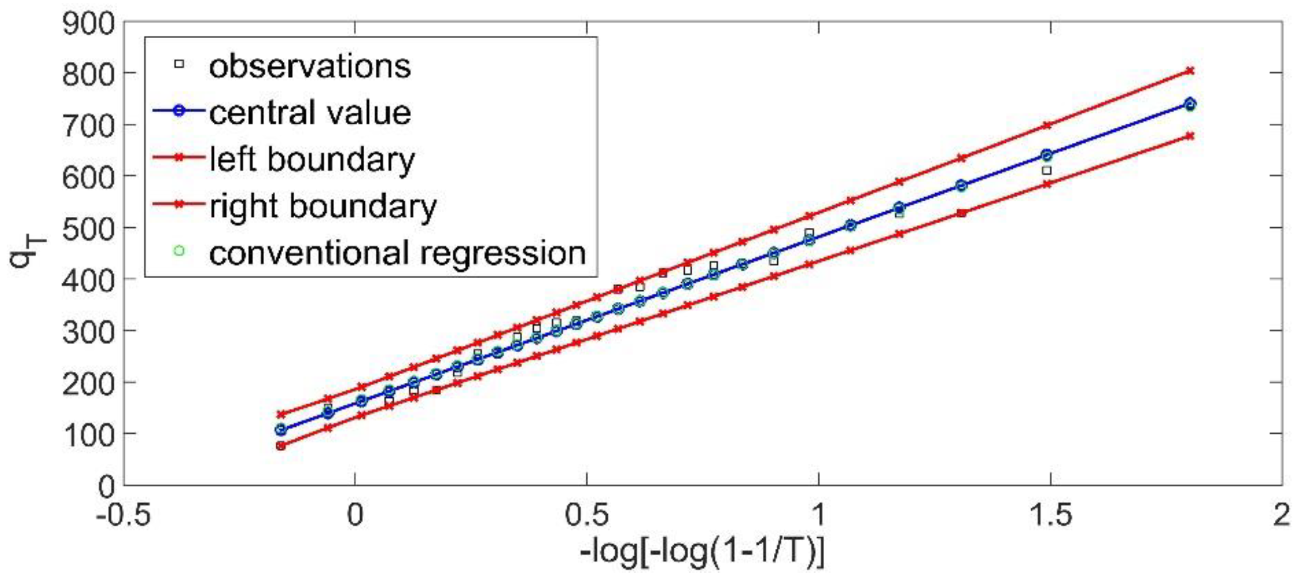
Secondly, the extreme value type I [
EV1(2)] theoretical distribution is examined. The fuzzy linear regression was applied (Tanaka et al. 1987) based on the aforementioned quantile approach, which leads to the following fuzzy curve:
while the sum of the produced semi-widths is:
Both fuzzy curves are depicted in
Figure 2 and
Figure 3. Based on the magnitude of the produced fuzzy band (that is, the value of the objective function), the GEV theoretical probability distribution is preferred. An interesting point is that every fuzzy linear regression problem based on the Tanaka methodology has a solution. The critical point is the magnitude of the produced fuzzy band. From
Figure 2 and
Figure 3, it is evident that the fuzzy band can be characterized as functional. Another important point of view is that all the data must be included within the produced fuzzy band, and hence all the empirical probabilities are within the produced fuzzy band.
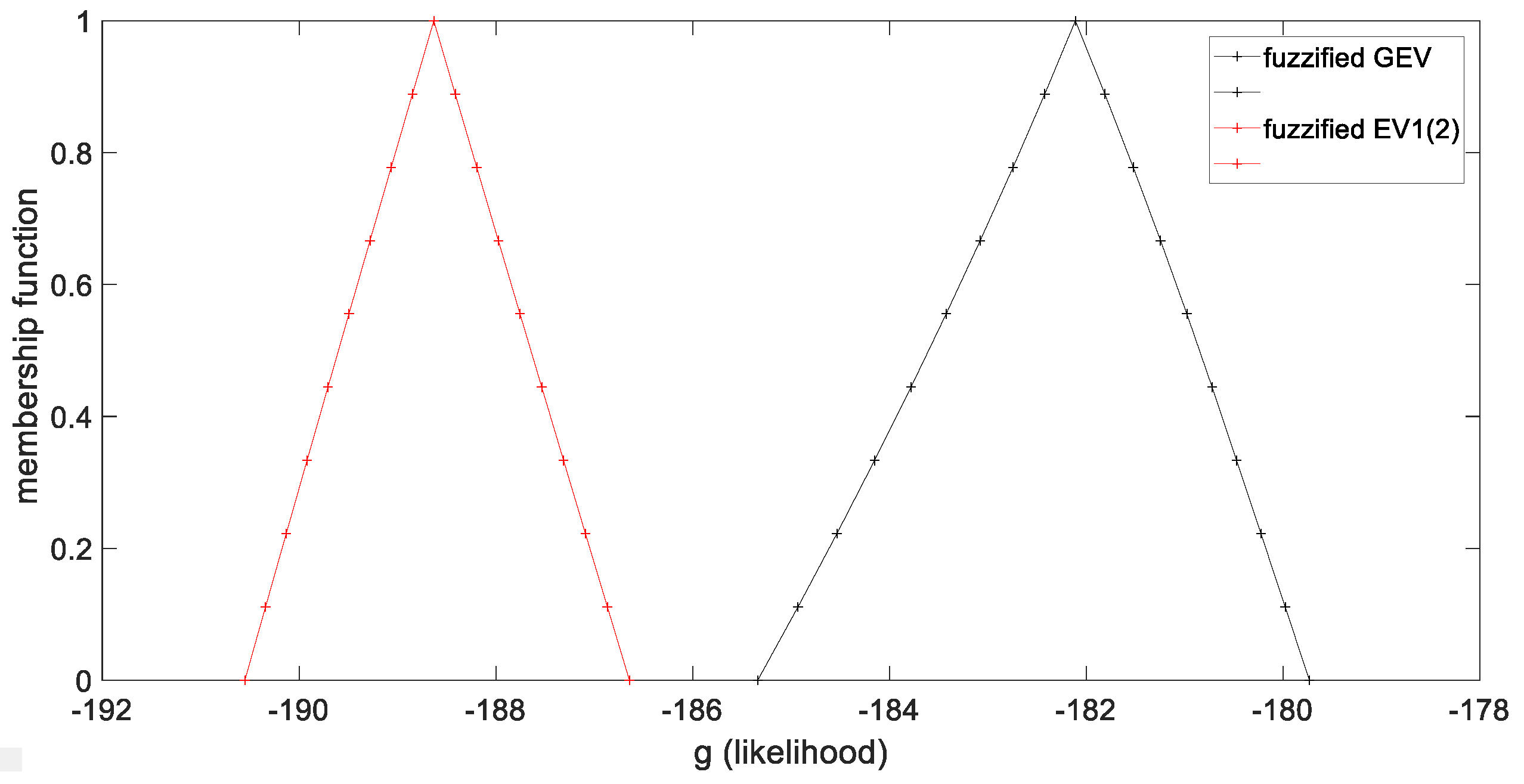
As mentionedbefore, the second measure of suitability is the produced fuzzy likelihood
g, which in its crisp expression, is a continuous function. Based on the extension principle (Equation (24)), the fuzzified likelihood is built by determining several α-cuts. The fuzzified likelihoods for both examined theoretical probability distributions are presented in
Figure 4. The two likelihoods have the shape of fuzzy numbers. Even if the comparison between two fuzzy numbers is an ill constructed problem, by applying several widely used measures, we conclude that the fuzzy likelihood of
GEV is greater than the fuzzy likelihood of
EV1(2) and hence the
GEV is preferred according to this criterion. We highlight that the fuzzified likelihood is determined based on the fuzzy regression, or in other words, the fuzzified likelihood is used as a suitability measure, and not in order to determine the parameters of the probability distribution.
4. Conclusions
In order to achieve the couple between the examined extreme theoretical probability distribution and the sample, a hybrid fuzzy regression based approach is developed. The fuzzy regression model is formulated according to the quantile approach, which relates the observed return period with the theoretical cumulative probability. The problem of fuzzy linear regression for crisp data and fuzzy triangular numbers as coefficients concludes to an equivalent linear programming problem.
Two theoretical probability distributions were applied to study the annual maximum river in Strymonas River: the GEV and the EV1(2). To evaluate the proposed approach, two measures of suitability are proposed. The first one is the magnitude of the produced fuzzy bands, which is the objective function regarding the equivalent optimization problem. The second measure is the fuzzified likelihood, which is built according to the extension principle and the solution of the fuzzy regression. It is concluded that, in both cases, a functional uncertainty appears; therefore, the use of the fuzzified theoretical probability function is successful and can be further utilized. Secondly, by comparing both objective functions and the fuzzified likelihood, the use of the fuzzified GEV must be preferred. Hence, the proposed measure of suitability can be used, in order to select the fuzzified theoretical probability function.


