GIS-Based Multi-Criteria Assessment and Seasonal Impact on Plantation Forest Landscape Visual Sensitivity


1
College of Landscape Architecture and Tourism, Hebei Agricultural University, NO.2596, Lekai South Street, Baoding 071000, China
2
National Long-term Scientific Research Base of Forest Cultivation in Saihanba of Hebei, Chengde 067000, China
3
College of Forestry, Hebei Agricultural University, NO.2596, Lekai South Street, Baoding 071000, China
*
Author to whom correspondence should be addressed.
Forests 2019, 10(4), 297; https://0-doi-org.brum.beds.ac.uk/10.3390/f10040297
Submission received: 2 March 2019
/
Revised: 26 March 2019
/
Accepted: 26 March 2019
/
Published: 30 March 2019
(This article belongs to the Section Forest Inventory, Modeling and Remote Sensing)
Abstract
:Visual sensitivity assessments identify the location of the high-sensitivity areas in terms of visual change. Studying the visual sensitivity of plantation forest landscapes and their seasonal changes can help resolve increasingly frequent conflicts between tourism and forest management activities, in the context of the multi-functional management of plantation forests. In this study, we used the geographic information system (GIS) and multi-criteria evaluation (MCE) methods combined with the analytic hierarchy process (AHP) to perform a visual sensitivity evaluation. Nine map-based criteria were selected, and the visual sensitivity of summer and autumn values were calculated, using data from sources including inventory data for forest management planning and design, digital elevation model (DEM), and aerial photographs. Vegetation uniformity (VU) and color diversity (CD) indices were constructed using three patch-level-based landscape indices, including area (AREA), fractal dimension index (FRAC), and proximity (PROX), to visualize the summer and autumn vegetation characteristics of a plantation forest landscape. We conducted a case study on the Saihanba Mechanical Forest Plantation, China’s largest forest plantation. The results were evaluated by experts, confirming the method to be reliable. This study provides an accurate, objective, and visualized evaluation method for the visual sensitivity of plantations for forest management units at the landscape scale. In analyzing the visual sensitivity of plantation forest landscapes, appropriate criteria, e.g., uniformity or diversity should be selected based on forest vegetation characteristics. When identifying high-sensitivity regions, it is necessary to simultaneously analyze areas with high visual sensitivity in different seasons and then superimpose the results.
1. Introduction
According to 2015 Food and Agriculture Organization (FAO) statistics, the world’s total plantation forests area is increasing [1]. With increased environmental protection pressure and greater demands for forest tourism and recreation, plantation forests have gradually shifted from a sole timber production function to multi-functional management, and from passive multi-functional utilization to active multi-functional operation [2]. The value of forest tourism and recreation has become an important aspect of the total value of the plantation forestry economy and an increasingly important determining factor in multi-functional forest operations [3]. People explore forests through multiple senses such as sight, hearing, taste, touch, and smell, of which vision is dominant [4]. A visually appealing forest landscape is not only conducive to tourism activities but also an environmental basis for various recreational activities [5,6,7,8].
Based on the possibility of human perception of human disturbance effects on a landscape, Litton (1974) proposed the concept of visual vulnerability, referring to the resilience and susceptibility levels of a landscape in response to the disturbances attributed to human activities and natural environmental changes [9]. In forest landscapes, visual sensitivity refers to the possibility of public attention and criticism caused by activities such as forest felling or land use change [10]. In high visual sensitivity areas, even a slight alteration might be easily perceived by the viewer. In the context of the multi-functional operation of the plantation forests, conflicts between sightseeing and forest management are becoming increasingly frequent [3,11,12]. It is important to identify the location of the most sensitive areas in terms of visual change. In addition, in plantation forests development, identical tree species and similarly sized saplings are often planted at standard distances, allowing forestry management measures to be easily implemented to achieve maximum economic benefits. Thus, plantation forests are primarily characterized as being single-layer forests that contain a single, predominantly coniferous tree species [13]; especially in summer, the visual perception is that of a large area of continuous forest with uniform color and texture, with very high visual sensitivity. However, the visual sensitivity of plantation forests has not been investigated in detail.
Initially, visual sensitivity was primarily evaluated through expert and field surveys [10,14]. Quantitative assessment of landscape quality [15,16,17] and visibility [18] using geographic information system (GIS) methods has simplified the complexity of landscapes and their perception, ensuring objectivity, replicability, and transparency of assessment results, thus facilitating the quantitatively assessment of visual sensitivity. GIS-based multi-criteria evaluation (MCE) coupled with the analytic hierarchy process (AHP) is a simple, effective, and comprehensive evaluation method [19,20] that is suitable for assessing the most sensitive areas [21]. Store et al. (2015) used this method to assess the visual sensitivity of forest landscapes at the regional scale and obtained reliable results [22]. However, this method has not been further tested at the level of forest management units, which, despite the small scale, would enable expert evaluations and field investigations to be easily conducted. Thus, the use of more objective, accurate, and visualized assessment methods for visual sensitivity can help better identify forest areas with high sensitivity.
The primary criteria affecting visual sensitivity include the number of users, their expectations and experiences, landscape attractiveness as determined by the physical characteristics of landscape organisms, and viewing condition, such as distance and visibility [10,14,23]. Thus, visual sensitivity may be assessed based on the amount and attention of users, landscape attractiveness, and viewing conditions, each reflecting the subject of viewing (viewer) and object (landscape), as well as the interaction between the two. It is generally considered that areas with high vegetation diversity also have high landscape attractiveness [15] and high visual sensitivity [23]. However, despite low diversity, in summer, plantation forest landscapes have very high visual sensitivity [10]. Therefore, it is necessary to investigate how to select criteria that appropriately reflect the visual sensitivity of plantation forest landscapes.
Seasonal changes may cause visual changes in land cover and land use, resulting in changes in landscape attractiveness [24]. Among these seasonal changes, the seasonal effect of vegetation is the most pronounced; for example, the exuberant color change of broad-leaved forests in the autumn increases landscape appeal [16]. However, some studies have shown that the research results regarding vegetation preferences for one season cannot be applied to another season [25], and that vegetation that is very attractive during the flowering season may have negative visual effects during the non-flowering season [26]. The effects of seasonal changes on urban landscapes [25,27] and agricultural landscapes [28,29] have been extensively investigated, whereas those on forest landscapes have been rarely studied. More importantly, landscape attractiveness is an important factor that influences visual sensitivity, and changes in landscape attractiveness may alter visual sensitivity. However, to the best of our knowledge, measurements of the effects of seasonal changes on visual sensitivity have not been investigated. If high visual sensitivity areas vary from season to season, then these areas should also be protected in other seasons. Therefore, in this study, we adopted the GIS-based MCE and AHP methods to establish an evaluation method for the visual sensitivity of plantation forest landscapes at the landscape scale of forest management units, and examined whether seasonal changes also cause changes in visual sensitivity.
2. Materials and Methods
2.1. Study Area
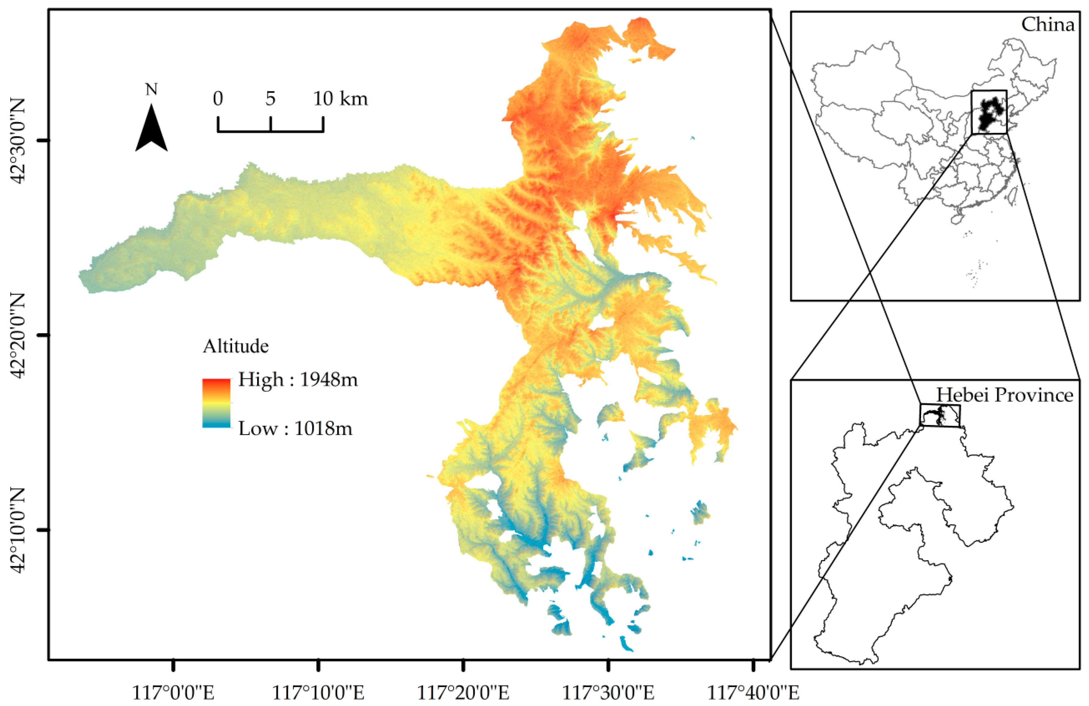
The Saihanba Mechanical Forest Plantation, located in the far north of Weichang Manchu and Mongolian Autonomous County of Chengde City, Hebei Province, is currently China’s largest forest plantation, with a total area of 92,634.7 ha. It is situated at the junction of the Inner Mongolia Plateau and the northern Hebei Mountains (116°51′ to 117°39′ E, 42°02′ to 42°36′ N), with an elevation ranging from 1018–1948 m (Figure 1). The area has a cold temperate continental monsoon climate: Long and cold winters characterized by seven months of snow coverage, short but dry and windy springs and autumns, and cool summers with an average temperature of 25 °C and intense sunlight. In the 1950s, the region resembled a wasteland because of rampant forest felling. Foresters revitalized the degraded land through afforestation. The forest coverage rate of the plantation is currently 75.5% now, forming a natural landscape dominated by forests, supplemented by wetlands, and mosaiced by rivers and lakes. The dominant tree species include Larix principis-rupprechtii Mayr., Pinus sylvestris var.mongoliac Litv., Picea asperata Mast., and Betula platyphylla Suk.. The Saihanba Mechanical Forest Plantation is a national forest park in China and won the “Champions of the Earth” award from the United Nations Environment Program in 2017. Forest tourism has become an important forestry industry, which receives 500,000 tourist visitors annually who predominantly engage in sightseeing, experiencing the astonishing view and the breeze from the vast forest in summer, and enjoying the colorful forest landscape in autumn. The tourism season usually typically begins in late June and is largely over by early October. Thus, two seasons (i.e., summer and autumn) were selected for this investigation.
2.2. Visual Sensitivity Assessment Procedures
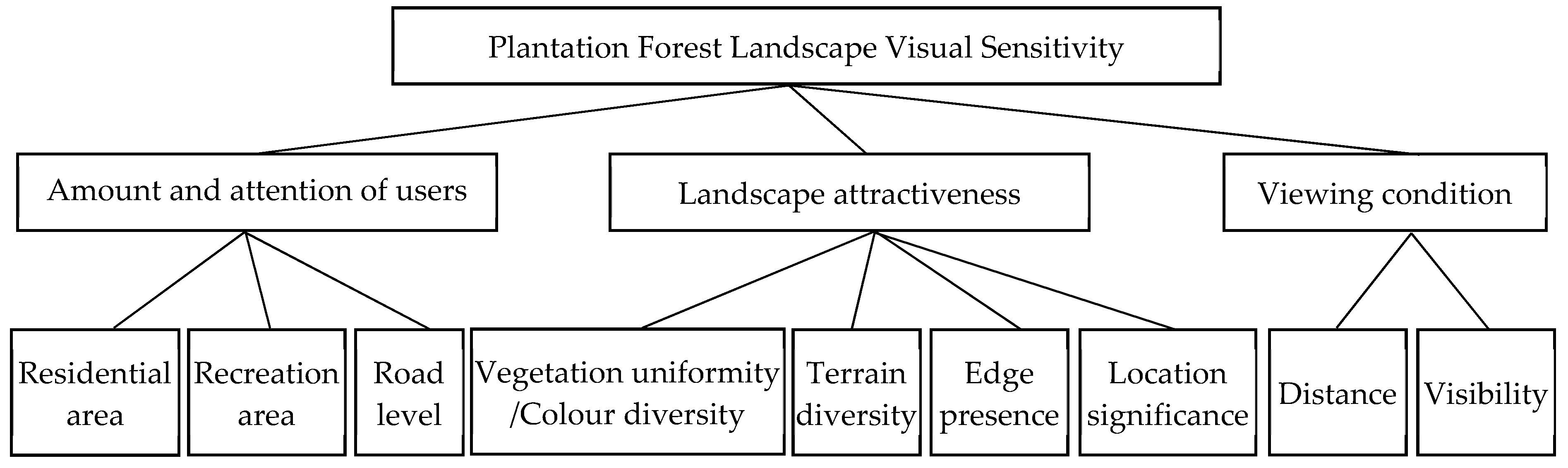
The GIS-based MCE and AHP methods were adopted for the comprehensive evaluation of visual sensitivity. Specific steps included the following: (1) A visual sensitivity assessment model was established based on the AHP concept and presented in a decision tree (Figure 2); (2) the criteria were evaluated by experts using pairwise comparison to obtain the weight of each criterion; (3) the criteria’s values were calculated using GIS software, and map layers for each criterion were generated; and (4) finally, using the synthesis model, the results of visual sensitivity assessment were produced and verified, and the high visual sensitivity areas were identified under different threshold values during summer and autumn.
2.3. Determination of the Sensitivity Creteria
According to a literature survey and expert consultations, three main criteria including the amount and attention of users, landscape attractiveness, and viewing condition [10,23], were selected based on the AHP concept to respectively reflect the effects of the subject (viewer), the object (landscape), and the interaction between the two in terms of visual sensitivity (Figure 2).
2.3.1. Amount and Attention of Users
Areas with high usage include residential areas, recreation areas, and roads, which also have high visual sensitivity. General residential areas are categorized into three types (i.e., accommodation area for visitors, forester living areas, and villages); the type of area with the highest visual sensitivity continues to be debated [23]. The recreation areas are characterized by unique landscape resources and have been developed due to the presence of more tourists and longer visit times, and thus have high visual sensitivity. The visual landscapes on both sides of a road are very important [30], and roads of different levels vary with regard to visual sensitivity [14]. Roads can be divided into two categories: major roads that connect recreation areas and minor roads that include other hard-surfaced roads within the forest management unit.
2.3.2. Landscape Attractiveness
Landscape attractiveness primarily measures the extent to which a landscape’s visual features, which are presented by the biophysical characteristics, attract people’s interests and attention [10]. The higher the landscape attractiveness, the higher the visual sensitivity. Areas with profound landscape attractiveness include lakes, which have typically been developed as recreation areas and were; therefore, not considered again to avoid obtaining excessively large values. Four aspects (i.e., vegetation, terrain, edge, and location) were selected as the sub-criteria [15,31].
Vegetation. During summer, in continuous, large-scale, plantation landscapes with uniform texture and color, the larger the patch area is, the higher the number of adjacent patches of the same type is, the higher the uniformity [31,32] or openness [31,33], and the higher the landscape attractiveness and visual sensitivity. In autumn, the canopies of different tree species exhibit different colors, and color diversity has become an important criterion for landscape attractiveness [34,35]. Additionally, in autumn, the boundaries and textures of patches are more distinctive. The more complex the patch shape is [36,37], the lower the number of the adjacent patches of the same type, the higher the color diversity, and the higher the landscape attractiveness and visual sensitivity. Thus, vegetation uniformity (VU) and color diversity (CD) were used to measure the visual characteristics of the plantation forests’ vegetation in summer and autumn.
Terrain. Terrain is of great importance in explaining the spatial structure of the landscape based on surface appearance and landscape elements [35,38], and terrain variety generate mystique and high landscape appeal because of morphological versatility and visual richness [39,40,41]. Therefore, terrain diversity was used to reflect landscape appeal and visual sensitivity.
Edge. Landscape edge refers to an interlaced zone of two or more adjacent landscapes, with heterogeneity as its most important feature [15], which exerts a positive effect on landscape attractiveness [42,43,44]. For example, the forest–lake landscape and the forest–meadow landscape both have stunning visual appeal with high visual sensitivity. Therefore, edge presence was used as a criterion.
Location. Specific topographic features (e.g., slope and aspect) also affect the extent attracting a viewer’s attention. Due to height differences and slope steepness, ridges are more attractive [45]; some ridges include the skyline, which is positively correlated with landscape attractiveness [33]. In the Northern Hemisphere, north-facing aspects are backlit and vistas are dark with lower color contrast; such inconspicuous lines and textures have lower visual sensitivity than south-facing aspects. Views of south-facing slopes are opposite to those of north-facing aspects [9,10]. Therefore, the more conspicuous the location is, the higher the landscape attractiveness. Thus, location significance was used as a criterion.
2.3.3. Viewing Condition
Viewing condition refers to the intermediate conditions under which the viewer observes the landscape, which is very important in visual sensitivity studies for determining which landscapes may be seen or are more clearly observed by the viewer. Visibility refers to whether the forest landscape may be seen by the viewer; the more often the forest landscape is seen by viewers, the higher the visual sensitivity of areas [18,46]. The closer the forest landscape is to viewers, the higher the visual sensitivity [14,47].
2.4. Determining the Weights of Criteria
Visual sensitivity is affected by multiple factors, and each factor has a different degree of influence; thus, it is necessary to determine the weight of each factor. The weight values were obtained using the AHP, in which the above criteria were included in an expert consultation questionnaire. The experts were asked to make pairwise comparisons of the criteria using the 1/9, 1/8, …, 1, …, 8, 9 scale, according to the consistent matrix method proposed by Saaty [48]. The 30 experts included 9 landscapes, 9 tourism, and 7 forestry experts, as well as 5 scientific and technical personnel from the forest plantation. In the calculation, a pairwise comparison matrix was created, and consistency index (CI) and consistency ratios (CR) were calculated. The CI was calculated according to the following formula:
where is the largest eigenvalue of the matrix, and n is the number of criteria in a comparison matrix. CI provides information on logical consistency among pairwise comparison judgments. CR is the ratio between CI and RI, and RI is a random consistency ratio generated by Saaty [49]. A CR of less than 0.1 indicated that the evaluation value passed the consistency test, and the weight was the geometric mean of each row of the matrix [49,50]. The calculation was conducted using the AHP package [51] in the R software [52].
2.5. Calculation and Mapping of Sub-Criteria
The calculation of sub-criteria was performed using the tools in the ArcGIS software (Esri, V10.1; Redlands, CA, USA), and the inventory data for management planning and design (2012, vector), the digital roads (vector), river and wetland maps (vector), the aerial images (recorded in 2012, 0.5 m resolution), and digital elevation model (DEM). In the calculation, the vegetation map and landcover map, which were the raster maps with resolution of 10 × 10 m, were generated based on these vector maps. The DEM of the study area obtained from ASTER GDEM V2 (Advanced Space-Borne Thermal Emission and Reflection Radiometer Global Digital Elevation Model Version 2, 30 × 30 m, 2011) was resampled to 10 × 10 m, then slope and aspect maps were generated based on it.
The min–max normalization was used to normalize the calculation result of each index in the range of 0 and 1. The values of four criteria (i.e., road level, vegetation, distance, and visibility) were calculated for summer and autumn.
The recreation areas and residential areas were digitized from aerial photographs. Buffer areas were set on roads, in which the buffer distance was the average tree height (approximately 25 m) plus the road width (approximately 10 m), forming a corridor 60 m in width. The tourist volume in recreation areas was higher than that in other areas and was thus valuated at 1 (0 for other areas). The experts were asked to perform pairwise comparisons on the importance of different residential areas and different levels of roads and generate respective evaluation values, as shown in Table 1; other areas were valuated at 0.
VU (vegetation uniformity) or CD (color diversity). Many studies have shown that the landscape pattern index can reflect visual characteristics of a landscape [31,53,54]. Three indices (i.e., area (AREA), fractal dimension index (FRAC), and proximity (PROX)), were selected to construct the VU (vegetation uniformity) or CD (color diversity) index using the following formulas:
, , and PROX = . In which is the area of the patch; is the perimeter of the patch; aijs is the area of patch ijs of the specific neighborhood of patch ij (m2); and hijs is the distance between patch ijs and ijs. When , the greater the is, the larger the patch area; when PROX ≥ 0, the greater the PROX, the higher the number of patches of the same type within a certain distance. When , the closer the is to 2, the more complex the patch shape. a, b, c, and d are parameters. The closer the VU is to 1, the higher the VU; the closer the CD is to 1, the higher the CD.
The AREA, FRAC, and PROX values were calculated using Fragstats software [55]. In the calculation, the vegetation in the summer was categorized into four categories (i.e., coniferous forest (L. gmelinii, P. sylvestris, P. asperata), broad-leaved forest (B. platyphylla, Quercus mongolica Fischer ex ledebour), shrubs, and grassland), of which the coniferous plantation and broad-leaved forests are visually different [42,56]. The vegetation in autumn was categorized into five categories (i.e., deciduous coniferous forest (L. gmelinii, yellow), evergreen coniferous forest (P. sylvestris, P. asperata, green), broad-leaved forest (yellow or red), shrubs, and grassland), of which the forest types largely differed in color in autumn. Other land use types occupy a relatively small proportion and were considered as background in the calculation.
The values of indices were calculated at the patch level [38], generating two files with the suffixes of patch and tif, respectively. The identifier and indices value of each patch were recorded in the patch file. The entropy weight of the indices can be calculated by the entropy method [57] using R software, which can be used as the parameter value of the index (Table 2). The patch identifiers and spatial information were recorded in the tif file. The patch file was joined with the tif file in ArcMap, and then the raster map of each index was generated with the resolution of 10 × 10 m. Then, the VU and CD were calculated according to their respective formulas.
Terrain diversity. Terrain diversity was measured using terrain relief and terrain roughness [58], both of which are macroscopic indicators that reflect surface morphology. When calculating terrain relief, neighborhood analysis was conducted on the DEM, and various windows of 3 × 3, 4 × 4..., 32 × 32 were calculated, in which the optimal window area was determined at 4.84 ha by change-point analysis [59]. The results were then converted to a floating-point grid and normalized, where the greater the value, the higher the relief.
Terrain roughness refers to the ratio of the surface area of the Earth to its projected area in a particular area. The greater the value is, the higher the terrain roughness [39,60]. The formula is as follows:
In which R represents terrain roughness and would be normalized. Terrain diversity superimposes terrain relief and terrain roughness with equal weights.
Edge presence. The lakes and wetlands were treated with a buffer analysis, in which the buffering distance was two times the average tree height. An analysis of the intersection with forests was performed, in which the forest edge with lakes and wetlands were calculated and valued at 1, and other areas were valued at 0.
Location significance. The topographic position index (TPI) comprehensively reflects height differences and slope [61], and the land facet corridor tool [62] was used to analyze the DEM. As the value increases, the slope is closer to the top of the mountain and thus has higher visual sensitivity. In the aspect analysis, the topographic solar radiation aspect (TRASP) index was used to convert the slope aspect (azimuth) to values ranging from 0–1 [63], in which 0 represents 30° east of north, and 1 represents 30° west of south. The closer the value is to 1, the drier and sunnier the habitat, and the higher the visual sensitivity. The formula is as follows:
In which Aspect is the azimuth. Location significance superimposes TPI and TRASP and both weights were 0.5.
Visibility. Points were distributed in 20-m intervals along trails in recreation areas and in 100-m intervals along major roads to form a viewpoint layer (Table 3), upon which viewshed analyses were performed using the cumulative viewshed method [64] and digital surface model (DSM) [42]. The DSM was calculated according to the following formula:
If the land use type was forests or shrubs, the height was the average height of the stand, which could be obtained from the data of inventory for forest management planning and design. The mean height of the accommodations area for visitors is 20 m, and that of villages is 4 m. When the DSM was used, blocking on the viewshed by surface factors such as vegetation was considered [39,42,65]. The viewpoints were categorized into two types [39], of which the majority of the viewpoints were horizontally-oriented with an offset height of 1.6 m, and some viewpoints were high above overlooking the forest landscape, and the offset heights were valuated based on the actual height difference as compared with the surrounding environment (Table 3).
DSM = [DEM] + [the height above level of DEM of each land use type]
Distance. The Euclidean distance tool was used to analyze the minimum distance between each grid point and the viewpoint in the study area. The effect of distance on visual sensitivity decreases linearly from the viewpoint and attenuates to 0 at the maximum distance. The valuation for the maximum distance is presented in Table 3.
2.6. Comprehensive Assessment and Model Validation
The arithmetic averaging method was selected as the synthesis model, which was achieved using the weighted sum tool in ArcMap. To facilitate understanding and comparison, the results were converted to values in the range of 0–100; the closer the value is to 100, the higher the visual sensitivity.
A verification questionnaire was formulated according to the method of Store et al. (2015) [22], and maps of 30 test quadrates (10 × 10m), including information on land cover, nearby roads, and recreation areas were generated, which were supplemented by aerial photographs (1:3000 in scale). The experts were asked to select the most sensitive quadrate (sensitivity value of 100) from all test squares and then provide the sensitivity value of other test quadrates relative to the most sensitive quadrate and each other. The questionnaires were distributed to the 30 experts who completed the index weight assessment, and questionnaire results were received from 10 experts.
The paired t-test was used to test whether visual sensitivity was significantly different between summer and autumn. Specifically, difference grids visual sensitivity was calculated for summer and autumn respectively using the raster calculator in ArcGIS. The mean and standard errors of each grid were obtained, from which the U statistic was calculated for the paired t-test.
High visual sensitivity areas are those that merit the most urgent attention, and they were calculated using the threshold values of μ + σ and μ + 2σ, in which μ is the mean visual sensitivity value and σ is the standard deviation of visual sensitivity values [66]. High visual sensitivity areas in summer and autumn should also be protected in other seasons; thus, they were superimposed to obtain the high visual sensitivity areas under different threshold values.
3. Results
3.1. Reliability
The test quadrates of means of the expert assessment and those calculated using the model were compared. The Pearson correlation coefficient between the two was 0.876 (p < 0.000), and the paired t-test result was to accept the null hypothesis (p = 0.086), indicating that the two were not different. Thus, the assessment model was very reliable.
3.2. Weight Values of Criteria
The weight of each criterion is shown in Table 4. Among the main criteria, the weight of landscape attractiveness was the highest, and among the sub-criteria, the weight of vegetation was the highest, and that of residential areas was the lowest.
3.3. Vegetation Uniformity and Color Diversity
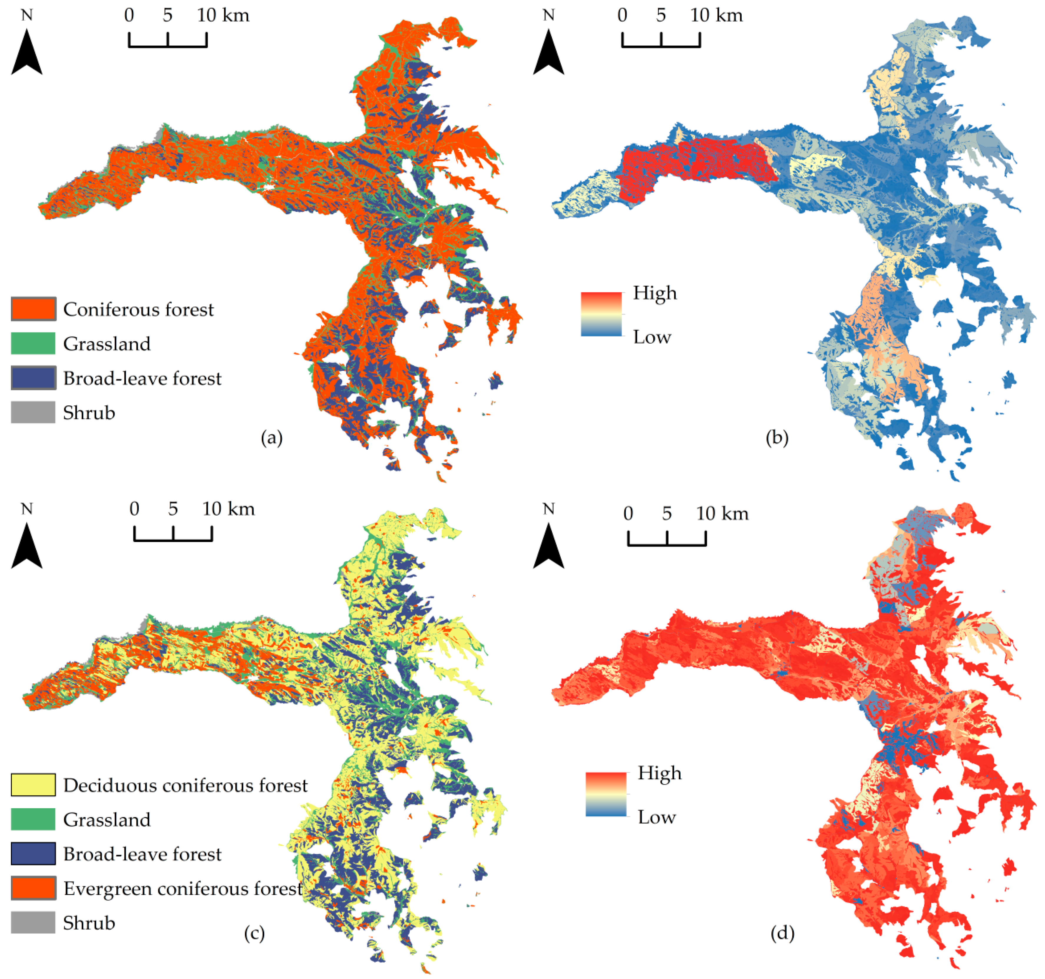
As shown in Figure 3, a comparison of the summer vegetation type map (a) and the VU map (b) indicates that areas with high VU were dominated by coniferous forests that have a larger patch area or a high number of adjacent patches of the same type, whereas those with low VU are the opposite. In autumn, the mix of evergreen coniferous forest patches and deciduous-coniferous forest patches, or the mix of deciduous-coniferous forest patches and broad-leaved forest patches (c) led to high CD in most areas, and areas with low CD were dominated by stands of purely deciduous-coniferous forests (d).
3.4. Assessment Results of Main Criteria
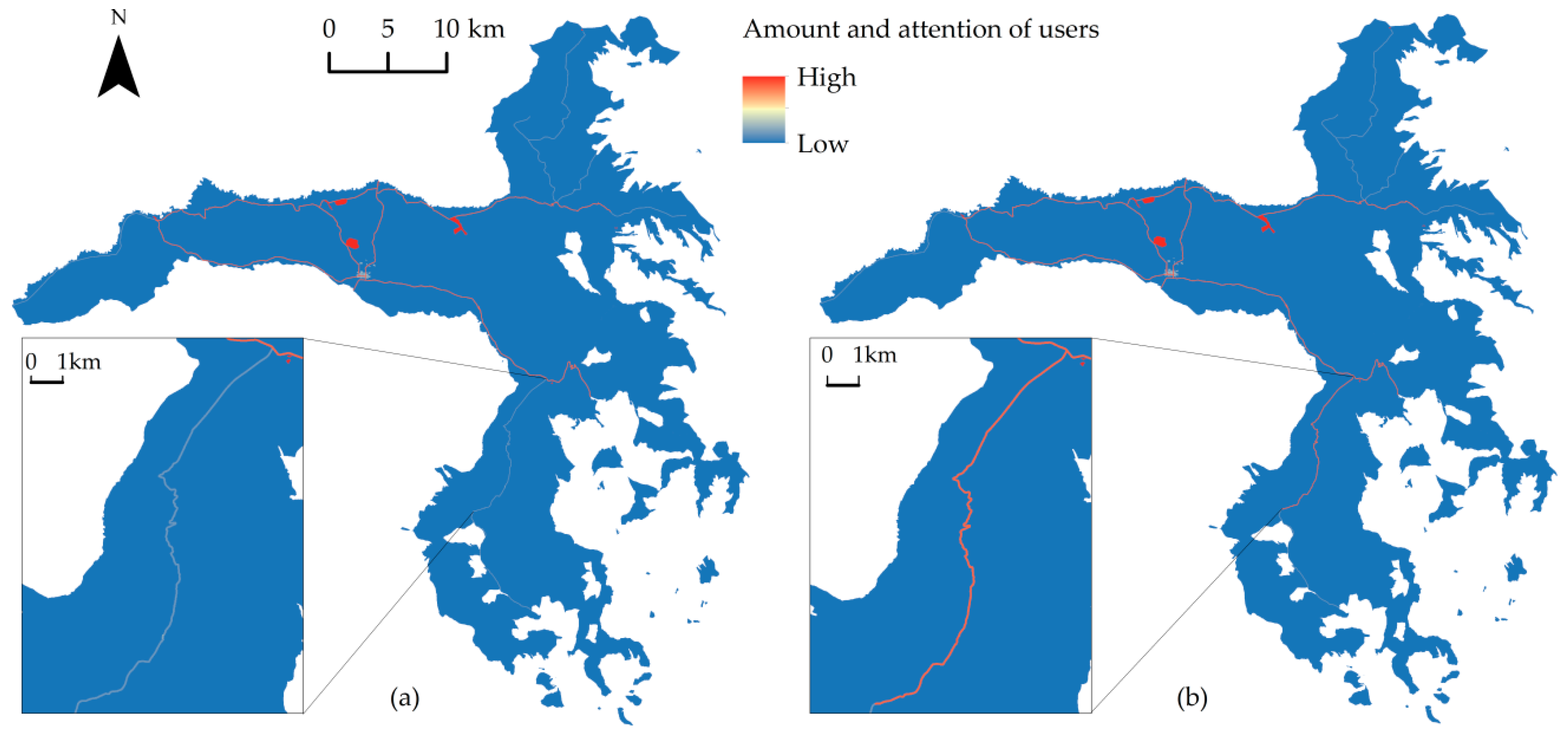
The analysis results on the amount and attention of users revealed some linear spaces (roads) and plane spaces (residential and recreation areas) in which viewers, especially tourists, gathered (Figure 4a,b). Compared to the situation in summer, the landscape on the two sides of a road segment approximately 15 km in length in autumn was superior; thus, the road was upgraded to a major road from a minor road in autumn, whereas the others remained unchanged.
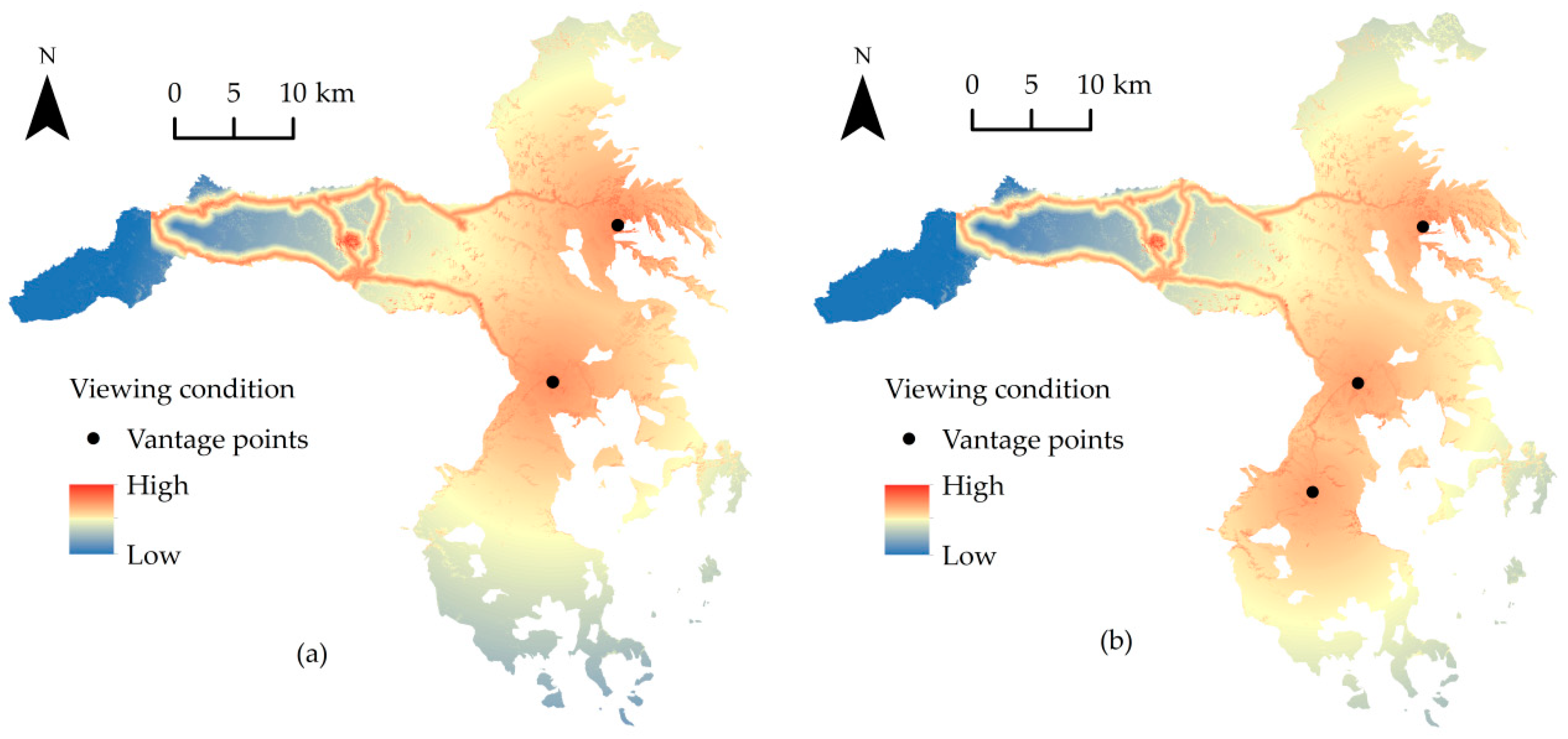
As shown in Figure 5, the distance from the overlooking viewpoints exerted a great effect on the results of the analysis of the viewing condition. Overlooking the forest landscape from a high viewpoint generated a vista and thus resulted in a higher visual sensitivity for the surrounding landscapes. Compared to that in summer, the addition of one overlooking viewpoint and the addition of 416 horizontally-oriented viewpoints along the above-described upgraded major road in autumn made little overall difference.
Figure 6a,b demonstrates that the spatial distributions of areas with high landscape attractiveness in summer and autumn were significantly different; they were characterized by a concentrated distribution in summer and scattered in autumn largely affected by vegetation.
3.5. Comprehensive Assessment
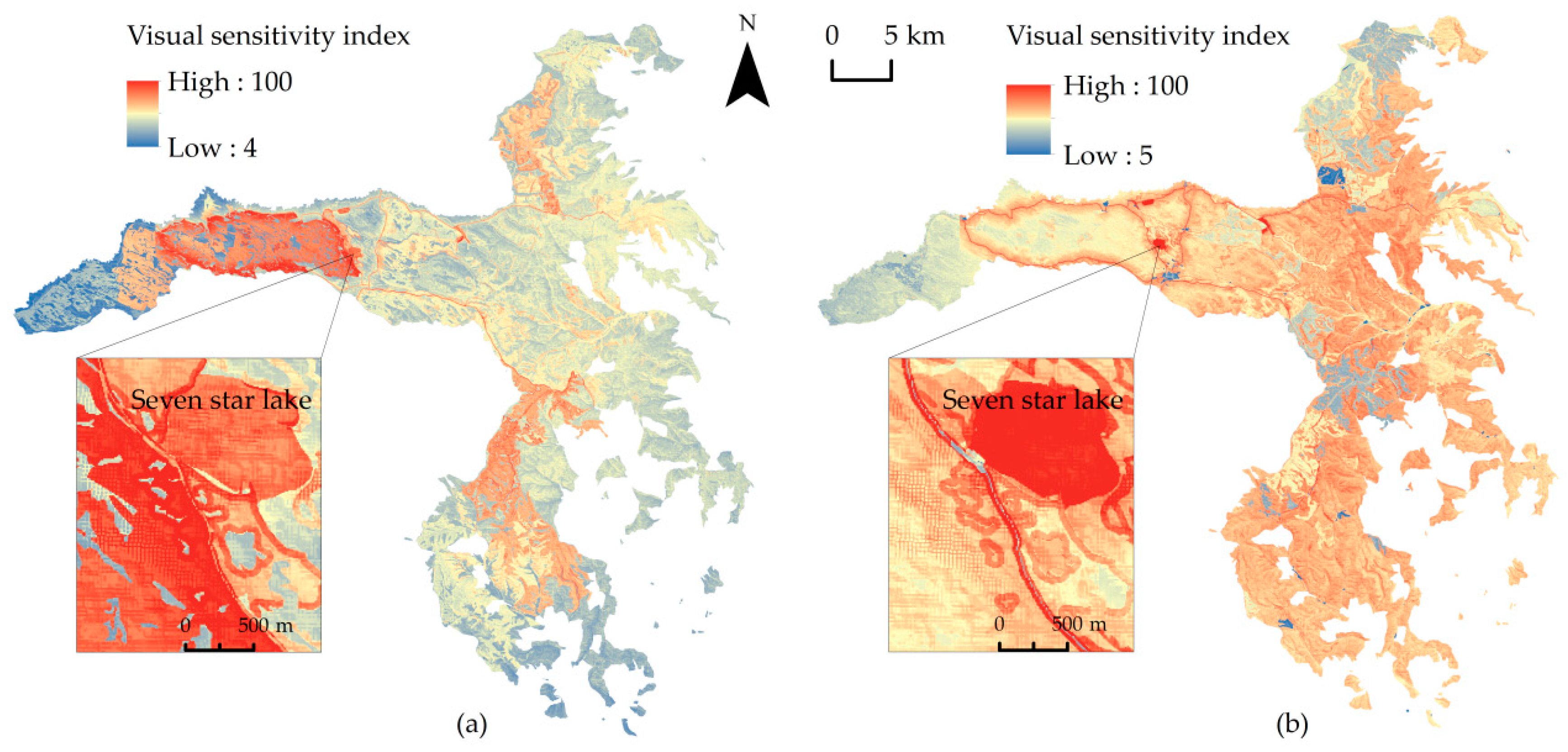
The mean value of visual sensitivity in summer was 33.5, with a standard deviation of 9.6, and that in autumn was 55.2, with a standard deviation of 7.5. As shown in Figure 7, the red color represents very sensitive and the blue color represents very insensitive. Summer and autumn significantly differed in visual sensitivity (). For example, the most famous recreation area, Seven Star Lake, had high-sensitivity values in both seasons. The dominated forest stands of the surrounding areas are pure plantation; thus, the sensitivity value was high in summer and low in autumn.
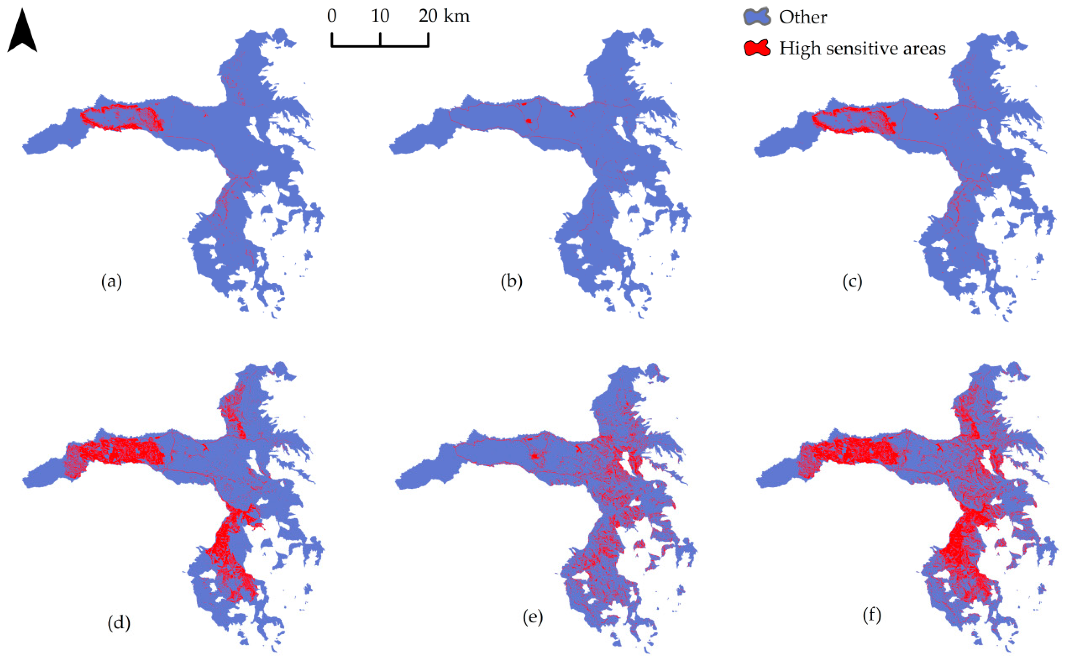
The high visual sensitivity areas under different thresholds in summer and autumn are presented in Figure 8. Under the two threshold conditions, the areas with high sensitivity in summer had a higher proportion than those in autumn. Under the threshold value of μ + 2σ, the superimposed areas with high sensitivity were primarily concentrated in recreation areas and on the two sides of the road. Under the threshold value of μ + σ, the areas with high sensitivity in summer were more concentrated, whereas those in autumn were more dispersed.
4. Discussion
In this study, we proposed a forest management unit-based comprehensive assessment method for the visual sensitivity of a plantation forest landscape. Through the AHP method, we constructed a visual sensitivity index system and obtained the weights of criteria, considering that each criterion had a different impact on visual sensitivity. The weight of vegetation was the highest, which is consistent with the reality of vegetation dominating the forest background. Forest vegetation also presented the highest weight in Store et al. (2015) [22].
The criteria were calculated based on a grid using the GIS, rather than on the landscape unit [14] or visual unit [10], making the assessment results more accurate [43]. Moreover, it is possible to calculate the value of any given unit (e.g., a compartment) using the zonal statistical tool of ArcMap. There are many defects in the multiple grading and synthesis of the criteria, such as the difficulty in ensuring accuracy [67]. In this study, we non-dimensionalized the criteria and adopted Boolean or continuous values, making it easy to operate the model and ensuring reliable results. In short, this method utilizes forest management units at the landscape-scale to accurately determine high visual sensitivity areas of plantation forest landscapes while visualizing them, such that the scope of multi-functional management dominated by visual landscape protection can be determined and conflicts with forest management can be avoided.
When considering landscape attractiveness and visual sensitivity, diversity was a common concept, and uniformity was often neglected. This paper emphasizes the importance of uniformity in the context of planted forests. The VU (vegetation uniformity) and CD (color diversity) criteria that were constructed based on the landscape pattern index at the patch level were purported to quantitatively and visually represent different visual features of vegetation in summer and autumn. Vegetation in summer and autumn differs in color and other formal elements, such as patch texture and boundaries, also vary; thus, different vegetation type maps and different indices were used in the calculation to reflect changes in the visual landscape in summer and autumn. Habitat types were used as a register of landscape change by Tasser, Ruffini, and Tappeiner (2009) [56]. Furthermore, VU and CD expressed spatial configuration among patches, whereas in previous studies, the index of the number of colors was used to express color diversity [34,41], and the index of the proportion of land use types changing with seasons was used to indicate seasonal change [30], both of which only reflected the landscape composition.
The value of the FRAC parameter in the CD formula was very low (0.02) because the value of the FRAC did not vary much (1.0–1.4) and the patches in the study area were predominantly geometric. Therefore, in plantation forestry environments, especially in areas of high sensitivity, patch shapes must be redesigned and modified to make them appear more natural, thus improving the landscape quality [68]. In this study, the intent was to measure visual sensitivity, but the high VU, high visual sensitivity, and poor visual adsorption capacity exhibited in the study area must be continuously improved in the future.
Landscapes in high visual sensitivity areas should be managed carefully. In this study, we presented high visual sensitivity areas under different threshold values, which can help forest management units prioritize visual landscape protection and management. The visual sensitivity map showed that under the threshold of μ + 2σ, areas with high sensitivity were primarily concentrated in recreation areas and along both sides of the major roads, which is in line with the findings of previous studies [22,69], where they were reported that areas with high sensitivity were located in areas of high usage. The high-sensitivity areas were also consistent with the spatial distribution of tourists. Compared with that of the foresters and local villagers, the visual sensitivity of areas of the tourist group was higher because tourists are more attracted to scenery [70]. The tourists were there for sightseeing, most visiting the forest plantation for the first time and leaving after staying in the forest plantation for half a day or a day. The recreation areas were the preferred locations to visit. Thus, the visual sensitivity of such areas was relatively high.
The increased high-sensitivity areas under the threshold of μ + σ, compared to μ + 2σ, had high landscape attractiveness or good viewing condition, most of them located in the middle and far zones of the viewshed, and contributing significantly to landscape quality [42]; thus, these areas also deserve more consideration, if possible.
The comparison of visual sensitivity in summer and autumn indicates that the two seasons differed significantly; thus, when analyzing visual sensitivity, seasonal impact should be considered. In previous studies, seasonality was not adequately studied, and visual sensitivity was investigated in only one season [22,65]. High visual sensitivity areas in different seasons should be superimposed to ensure that high visual sensitivity areas for one season are also protected in other seasons.
Because there are fewer visitors in winter and spring, it is of little significance to evaluate visual sensitivity during these seasons [9]. In this study, we only examined the visual sensitivity during two seasons; however, with the increasing number of tourists in winter, it is necessary to examine the visual sensitivity. The data used in this study were the most recent data from the study area, and the field survey indicated that the data used in the study (landcover, terrain, etc.) remained unchanged due to strict state-owned forest land-use policies. Nevertheless, the described research method could support updating results quickly as data changes.
5. Conclusions
In this study, we conducted a quantitative, accurate, and visualized assessment of the visual sensitivity of plantation forest landscapes using nine map-based criteria (residential areas, recreation areas, roads, VU or CD, terrain diversity, edge presence, location significance, distance, and visibility) based on three aspects, including amount and attention of users, landscape attractiveness, and viewing condition, using the GIS-based MCE coupled with the AHP. This model can help forest management units determine the visual landscapes that require priority protecting in the context of multi-functional management, avoiding the impact of forest harvesting on visual landscapes, while helping to select planting designs and afforestation treatments that meet tourists’ preferences.
In the forest background, forest vegetation is the primary cause of differences in visual sensitivity. In analyzing the visual sensitivity of plantation landscapes, selecting appropriate criteria based on the characteristics of forest vegetation is recommended. For example, in the case of a forest landscape in autumn or a mixed forest landscape, more importance is assigned to diversity, whereas in the case of a forest landscape in summer or a pure forest landscape, more importance is assigned to uniformity; otherwise, the visual sensitivity may be misjudged.
The comparison of visual sensitivity in summer and autumn using the above method indicated that the two seasons differed significantly. Therefore, it is necessary to analyze high visual sensitivity areas and superimpose them to ensure that the visual resources of high-sensitivity areas are not disturbed with in other seasons.
Author Contributions
H.Y. and H.X. conceived and designed the methodology, analyzed the data, and wrote the paper. L.Y. performed data collection; Z.Z. and X.Z. reviewed and edited.
Funding
This research was funded by the National Key Research and Development Plan, No. 2017YFD0600403 and the National Science Foundation of China, No.31370636.
Acknowledgments
We thank the Saihanba Mechanical Forest Plantation in Hebei Province for providing data and investigation convenience and are grateful to all of the experts for their support in selecting indicators, determining the weights, and verifying the results.
Conflicts of Interest
The authors declare no conflict of interest.
References
- Keenan, R.; Reams, G.; Achard, F.; de Freitas, J.; Grainger, A.; Lindquist, E. Dynamics of Global Forest Area: Results from the FAO Global Forest Resources Assessment 2015. For. Ecol. Manag. 2015, 352, 9–20. [Google Scholar] [CrossRef]
- Lu, Y. Supporting Precision Improvement Project of Forest Quality with Multifunctional Management Technology. Land Green. 2017, 4, 22–25. [Google Scholar]
- Eggers, J.; Lindhagen, A.; Lind, T.; Lämås, T.; Öhman, K. Balancing Landscape-level Forest Management between Recreation and Wood Production. Urban For. Urban Green. 2018, 33, 1–11. [Google Scholar] [CrossRef]
- Recreation Branch, BC Ministry of Forests (BCMoF) (Ed.) Visual Landscape Design Training Manual; Recreation Branch Publication: Victoria, BC, Canada, 1994; p. 5. ISBN 0-7726-2437-2.
- Abildtrup, J.; Garcia, S.; Olsen, S.B.; Stenger, A. Spatial Preference Heterogeneity in Forest Recreation. Ecol. Econ. 2013, 92, 67–77. [Google Scholar] [CrossRef]
- Agimass, F.; Lundhede, T.; Panduro, T.E.; Jacobsen, J.B. The Choice of Forest Site for Recreation: A Revealed Preference Analysis Using Spatial Data. Ecosyst. Serv. 2018, 31, 445–454. [Google Scholar] [CrossRef]
- Arnberger, A.; Schneider, I.E.; Ebenberger, M.; Eder, R.; Venette, R.C.; Snyder, S.A.; Gobster, P.H.; Choi, A.; Cottrell, S. Emerald Ash Borer Impacts on Visual Preferences for Urban Forest Recreation Settings. Urban For. Urban Green. 2017, 27, 235–245. [Google Scholar] [CrossRef]
- Eriksson, L.; Nordlund, A.; Olsson, O.; Westin, K. Recreation in Different Forest Settings: A Scene Preference Study. Forests 2012, 4, 923–943. [Google Scholar] [CrossRef]
- Litton, R.B. Visual Vulnerability of Forest Landscapes. J. For. 1974, 7, 392–397. [Google Scholar]
- Forest Practices Branch, BC Ministry of Forests (BCMoF) (Ed.) Visual Landscape Inventory:Procedures and Standards Manual; Forest Practices Branch, BC Ministry of Forests (BCMoF): Victoria, BC, Canada, 1997.
- Ode, Å.; Fry, G.; Tveit, M.S.; Messager, P.; Miller, D. Indicators of Perceived Naturalness as Drivers of Landscape Preference. J. Environ. Manag. 2009, 90, 375–383. [Google Scholar] [CrossRef]
- Gundersen, V.S.; Frivold, L.H. Public Preferences for Forest Structures: A Review of Quantitative Surveys from Finland, Norway and Sweden. Urban For. Urban Green. 2008, 7, 241–258. [Google Scholar] [CrossRef]
- Nielsen, A.B.; Jensen, R.B. Some Visual Aspects of Planting Design and Silviculture across Contemporary Forest Management Paradigms—Perspectives for Urban Afforestation. Urban For. Urban Green. 2007, 6, 143–158. [Google Scholar] [CrossRef]
- Forest Service (Ed.) Landscape Aesthetics: A Handbook of Scenery Management; U.S. Government Printing Office: Washington, DC, USA, 1995.
- Dronova, I. Environmental Heterogeneity as a Bridge between Ecosystem Service and Visual Quality Objectives in Management, Planning and Design. Landsc. Urban Plan. 2017, 163, 90–106. [Google Scholar] [CrossRef]
- Dramstad, W.E.; Tveit, M.S.; Fjellstad, W.J.; Fry, G.L. Relationships between Visual Landscape Preferences and Map-based Indicators of Landscape Structure. Landsc. Urban Plan. 2006, 78, 465–474. [Google Scholar] [CrossRef]
- Bishop, I.D.; Hulse, D.W. Prediction of Scenic Beauty Using Mapped Data and Geographic Information Systems. Landsc. Urban Plan. 1994, 30, 59–70. [Google Scholar] [CrossRef]
- Nutsford, D.; Reitsma, F.; Pearson, A.L.; Kingham, S. Personalising the Viewshed: Visibility Analysis from the Human Perspective. Appl. Geogr. 2015, 62, 1–7. [Google Scholar] [CrossRef]
- Chandio, I.A.; Matori, A.N.B.; WanYusof, K.B.; Talpur, M.A.H.; Balogun, A.-L.; Lawal, D.U. GIS-based Analytic Hierarchy Process as a Multicriteria Decision Analysis Instrument: A Review. Arab. J. Geosci. 2013, 6, 3059–3066. [Google Scholar] [CrossRef]
- Ananda, J.; Herath, G. A Critical Review of Multi-criteria Decision Making Methods with Special Reference to Forest Management and Planning. Ecol. Econ. 2009, 68, 2535–2548. [Google Scholar] [CrossRef]
- Mosadeghi, R.; Warnken, J.; Tomlinson, R.; Mirfenderesk, H. Comparison of Fuzzy-AHP and AHP in a Spatial Multi-criteria Decision Making Model for Urban Land-use Planning. Comput. Environ. Urban Syst. 2015, 49, 54–65. [Google Scholar] [CrossRef]
- Store, R.; Karjalainen, E.; Haara, A.; Leskinen, P.; Nivala, V. Producing a Sensitivity Assessment Method for Visual Forest Landscapes. Landsc. Urban Plan. 2015, 144, 128–141. [Google Scholar] [CrossRef]
- Haara, A.; Store, R.; Leskinen, P. Analyzing Uncertainties and Estimating Priorities of Landscape Sensitivity Based on Expert Opinions. Landsc. Urban Plan. 2017, 163, 56–66. [Google Scholar] [CrossRef]
- Tveit, M.S.; Ode, Å.; Fry, G. Key Concepts in a Framework for Analysing Visual Landscape Character. Landsc. Res. 2006, 31, 229–255. [Google Scholar] [CrossRef]
- Gerstenberg, T.; Hofman, M. Perception and Preference of Trees: A Psychological Contribution to Tree Species Selection in Urban Areas. Urban For. Urban Green. 2016, 15, 103–111. [Google Scholar] [CrossRef]
- Jorgensen, A.; Hitchmough, J.; Calvert, T. Woodland Spaces and Edges: Their Impact on Perception of Safety and Preference. Landsc. Urban Plan. 2002, 66, 135–150. [Google Scholar] [CrossRef]
- Zhao, J.; Xu, W.; Li, R. Visual Preference of Trees: The Effects of Tree Attributes and Seasons. Urban For. Urban Green. 2017, 25, 19–25. [Google Scholar] [CrossRef]
- Junge, X.; Schüpbach, B.; Walter, T.; Schmid, B.; Lindemann-Matthies, P. Aesthetic Quality of Agricultural Landscape Elements in Different Seasonal Stages in Switzerland. Landsc. Urban Plan. 2015, 133, 67–77. [Google Scholar] [CrossRef]
- Schupbach, B.; Junge, X.; Lindemann-Matthies, P.; Walter, T. Seasonality, Diversity and Aesthetic Valuation of Landscape Plots: An Integrative Approach to Assess Landscape Quality on Different Scales. Land Use Policy 2016, 53, 27–35. [Google Scholar] [CrossRef]
- Martín, B.; Ortega, E.; Otero, I.; Arce, R.M. Landscape Character Assessment with GIS Using Map-based Indicators and Photographs in the Relationship between Landscape and Roads. J. Environ. Manag. 2016, 180, 324–334. [Google Scholar] [CrossRef] [PubMed]
- Fry, G.; Tveit, M.S.; Ode, Å.; Velarde, M.D. The Eology of Visual Landscape: Exploring the Conceptual Common Ground of Visual and Ecological Landscape Indicators. Ecol. Indic. 2009, 9, 933–947. [Google Scholar] [CrossRef]
- Palme, J.F. Using Spatial Metrics to Predict Scenic Perception in a Changing Landscape: Dennis, Massachusetts. Landsc. Urban Plan. 2004, 69, 201–208. [Google Scholar] [CrossRef]
- Sahraoui, Y.; Clauzel, C.; Foltete, J.-C. Spatial Modelling of Landscape Aesthetic Potential in Urban-rural Fringes. J. Environ. Manag. 2016, 181, 623–636. [Google Scholar] [CrossRef]
- Polat, A.T.; Akay, A. Relationships between the Visual Preferences of Urban Recreation Area Users and Various Landscape Design Elements. Urban For. Urban Green. 2015, 14, 573–582. [Google Scholar] [CrossRef]
- Acar, C.; Sakıcı, Ç. Assessing Landscape Perception of Urban Rocky Habitats. Build. Environ. 2008, 6, 1153–1170. [Google Scholar] [CrossRef]
- Saura, S.; Torras, O.; Gil-Tena, A.; Pascual-Hortal, L. Shape Irregularity as an Indicator of Forest Biodiversity and Guidelines for Metric Selection. In Patterns and Processes in Forest Landscapes; Lafortezza, R., Sanesi, G., Chen, J., Crow, T.R., Eds.; Springer: Dordrecht, Holland, 2008; pp. 167–189. ISBN 978-1-4020-8503-1. [Google Scholar]
- Ode, Å.; Tveit, M.S.; Fry, G. Advantages of Using Different Data Sources in Assessment of Landscape Change and Its Effect on Visual Scale. Ecol. Indic. 2010, 10, 24–31. [Google Scholar] [CrossRef]
- Appleton, J. The Experience of Landscape; Wiley: London, UK, 1975; pp. 95–96. ISBN 9780471962359. [Google Scholar]
- Swetnam, R.D.; Harrison-Curran, S.K.; Smitha, G.R. Quantifying Visual Landscape Quality in Rural Wales: A GIS-enabled Method for Extensive Monitoring of a Valued Cultural Ecosystem Service. Ecosyst. Serv. 2017, 26, 451–464. [Google Scholar] [CrossRef]
- García-Llorente, M.; Martín-López, B.; Iniesta-Arandia, I.; López-Santiago, C.A.; Aguilera, P.A.; Montes, C. The Role of Multi-functionality in Social Preferences toward Semi-arid Rural Landscapes: An Ecosystem Service Approach. Environ. Sci. Policy 2012, 19, 136–146. [Google Scholar] [CrossRef]
- Arriaza, M.; Cañas-Ortega, J.F.; Cañas-Madueño, J.A.; Ruiz-Aviles, P. Assessing the Visual Quality of Rural Landscapes. Landsc. Urban Plan. 2004, 69, 115–125. [Google Scholar] [CrossRef]
- Schirpke, U.; Tasser, E.; Tappeiner, U. Predicting Scenic Beauty of Mountain Regions. Landsc. Urban Plan. 2013, 111, 1–12. [Google Scholar] [CrossRef]
- Herbst, H.; Förster, M.; Kleinschmit, B. Contribution of Landscape Metrics to the Assessment of Scenic Quality—The Example of the Landscape Structure Plan Havelland/Germany. Landsc. Online 2009, 10, 1–17. [Google Scholar] [CrossRef]
- Hammitt, W.E.; Patterson, M.E.; Noe, F.P. Identifying and Predicting Visual Preference of Southern Appalachian Forest Recreation Vistas. Landsc. Urban Plan. 1994, 29, 171–183. [Google Scholar] [CrossRef]
- Sklenicka, P.; Zouhar, J. Predicting the Visual Impact of Onshore Wind Farms via Landscape Indices: A Method for Objectivizing Planning and Decision Processes. Appl. Energy 2018, 209, 445–454. [Google Scholar] [CrossRef]
- Chamberlain, B.C.; Meitner, M.J. A Route-based Visibility Analysis for Landscape Management. Landsc. Urban Plan. 2013, 111, 13–24. [Google Scholar] [CrossRef]
- De Vries, S.; de Groot, M.; Boers, J. Eyesores in Sight: Quantifying the Impact of Man-made Elements on the Scenic Beauty of Dutch Landscapes. Landsc. Urban Plan. 2012, 105, 118–127. [Google Scholar] [CrossRef]
- Saaty, T.L. A Scaling Method for Priorities in Hierarchical Structures. J. Math. Psychol. 1977, 3, 234–281. [Google Scholar] [CrossRef]
- Saaty, T.L. Relative Measurement and Its Generalization in Decision Making Why Pairwise Comparisons are Central in Mathematics for the Measurement of Intangible Factors the Analytic Hierarchy/Network Process. Rev. R. Acad. Cien. Serie. A. Mat. 2008, 102, 251–318. [Google Scholar] [CrossRef]
- Pradhan, A.M.S.; Kim, Y.T. Evaluation of a Combined Spatial Multi-criteria Evaluation Model and Deterministic Model for Landslide Susceptibility Mapping. Catena 2016, 140, 125–139. [Google Scholar] [CrossRef]
- Caha, J.; Drážná, A. R Package for Calculation of (Fuzzy) AHP, Version 0.9.1. Available online: http://github.com/JanCaha/FuzzyAHP/ (accessed on 10 August 2018).
- R i386 3.5.1. Available online: https://www.r-project.org/ (accessed on 8 August 2018).
- De Val, G.D.; Atauri, J.A.; de Lucio, J.V. Relationship between Landscape Visual Attributes and Spatial Pattern Indices: A Test Study in Mediterranean-climate Landscapes. Landsc. Urban Plan. 2006, 77, 393–407. [Google Scholar] [CrossRef]
- Sowińska-Świerkosz, B. Index of Landscape Disharmony (ILDH) as a New Tool Combining the Aesthetic and Ecological Approach to Landscape Assessment Barbara. Ecol. Indic. 2016, 70, 166–180. [Google Scholar] [CrossRef]
- McGarigal, K.; Cushman, S.A.; Ene, E. FRAGSTATS v4: Spatial Pattern Analysis Program for Categorical and Continuous Maps. 2012. Available online: http://www.umass.edu/landeco/research/fragstats/fragstats.html (accessed on 6 July 2018).
- Tasser, E.; Ruffini, F.V.; Tappeiner, U. An Integrative Approach for Analysing Landscape Dynamics in Diverse Cultivated and Natural Mountain Areas. Landsc. Ecol. 2009, 5, 611–628. [Google Scholar] [CrossRef]
- Xu, H.; Ma, C.; Lian, J.; Xu, K.; Chaima, E. Urban Flooding Risk Assessment Based on an Integrated k-means Cluster Algorithm and Improved Entropy Weight Method in the Region of Haikou, China. J. Hydrol. 2018, 563, 975–986. [Google Scholar] [CrossRef]
- Marchi, L.; Cavalli, M.; Trevisani, S. Hypsometric Analysis of Headwater Rock Basins in the Dolomites (Eastern Alps) Using High-Resolution Topography. Geogr. Ann. 2015, 97, 317–335. [Google Scholar] [CrossRef]
- Han, H.; Gao, T.; Yi, H.; Yang, M.; Yan, X.; Ren, G.; Yang, J. Extraction of Relief Amplitude Based on Change Point Method: A Case Study on the Tibetan Plateau. Sci. Geogr. Sin. 2012, 32, 101–104. [Google Scholar]
- Berti, M.; Corsini, A.; Daehne, A. Comparative Analysis of Surface Roughness Algorithms for the Identification of Active Landslides. Geomorphology 2013, 182, 1–18. [Google Scholar] [CrossRef]
- Weiss, A.D. Topographic Position and Landforms Analysis. In Proceedings of the ESRI International User Conference, San Diego, CA, USA, 9–13 July 2001. [Google Scholar]
- Jenness, J. Land Facet Corridor Designer for ArcGIS 10, Revision 1.2.884. Available online: http://www.jennessent.com/arcgis/arcgis_extensions.htm (accessed on 5 May 2018).
- Roberts, D.W.; Cooper, S.V. Concepts and Techniques of Vegetation Mapping. In Land Classifications Based on Vegetation: Applications for Resource Management; General Technical Report INT_257; USDA, Forest Service, Intermountain Research Station: Ogden, UT, USA, 1989; pp. 90–96. [Google Scholar]
- 5.9.2. Cumulative Viewshed Analysis and Exposure Index. 2015. Available online: http://mapaspects.org/book/export/html/2134 (accessed on 8 June 2018).
- Scarfò, F.; Mercurio, R.; Del Peso, C. Assessing Visual Impacts of Forest Operations on a Landscape in the Serre Regional Park of Southern Italy. Landsc. Ecol. Eng. 2013, 9, 1–10. [Google Scholar] [CrossRef]
- Selim, S.; Koc-San, D.; Selim, C.; San, B.T. Site Selection for Avocado Cultivation Using GIS and Multi-criteria Decision Analyses: Case Study of Antalya, Turkey. Comput. Electron. Agric. 2018, 154, 450–459. [Google Scholar] [CrossRef]
- Su, W.H. Research on Theory and Method of Multi-Index Comprehensive Evaluation. Ph.D. Thesis, Xiamen University, Xiamen, China, 2000. [Google Scholar]
- Frank, S.; Fürst, C.; Koschkea, L.; Witta, A.; Makeschin, F. Assessment of Landscape Aesthetics—Validation of a Landscape Metrics-based Assessment by Visual Estimation of the Scenic Beauty. Ecol. Indic. 2013, 32, 222–231. [Google Scholar] [CrossRef]
- Tang, X. RS-GIS Based Fuzzy Evaluation of Landscape Visual Sensitivity of Three Gorges of Yangtze River. J. Tongji Univ. (Nat. Sci.) 2008, 36, 1679–1685. [Google Scholar]
- Deng, J.; Andrada, R.; Pierskalla, C. Visitors’ and Residents’ Perceptions of Urban Forests for Leisure in Washington D.C. Urban For. Urban Green. 2017, 28, 1–11. [Google Scholar] [CrossRef]
Figure 1.
The location and hill-shade map of Saihanba Mechanical Forest Plantation.

Figure 2.
Criteria tree for determining the visual sensitivity of the plantation forest landscape.

Figure 3.
Relationship between vegetation and VU (vegetation uniformity), CD (color diversity) of Saihanba Mechanical Forest Plantation: (a) Summer vegetation map; (b) summer VU map; (c) autumn vegetation map; and (d) autumn CD map.
Figure 3.
Relationship between vegetation and VU (vegetation uniformity), CD (color diversity) of Saihanba Mechanical Forest Plantation: (a) Summer vegetation map; (b) summer VU map; (c) autumn vegetation map; and (d) autumn CD map.

Figure 4.
Map of the main criteria, amount and attention of users of Saihanba Mechanical Forest Plantation, in (a) summer and (b) autumn.
Figure 4.
Map of the main criteria, amount and attention of users of Saihanba Mechanical Forest Plantation, in (a) summer and (b) autumn.

Figure 5.
Map of the main criteria, viewing condition of Saihanba Mechanical Forest Plantation, in (a) summer and (b) autumn.
Figure 5.
Map of the main criteria, viewing condition of Saihanba Mechanical Forest Plantation, in (a) summer and (b) autumn.

Figure 6.
Map of the main criteria, landscape attractiveness of Saihanba Mechanical Forest Plantation, in (a) summer and (b) autumn.
Figure 6.
Map of the main criteria, landscape attractiveness of Saihanba Mechanical Forest Plantation, in (a) summer and (b) autumn.

Figure 7.
Map of the visual sensitivity index of Saihanba Mechanical Forest Plantation in (a) summer and (b) autumn.
Figure 7.
Map of the visual sensitivity index of Saihanba Mechanical Forest Plantation in (a) summer and (b) autumn.

Figure 8.
High-sensitivity areas under the threshold value of μ+ 2σ (a) in summer accounts for 3.9%; (b) in autumn accounts for 1.0%; (c) the superimposed area accounts for 4.6%; and under the threshold value of μ + σ (d) in summer accounts for 19.6%; (e) in autumn accounts for 10.9%; (f) the superimposed area accounts for 25.3%.


Table 1.
Values of residential areas and roads obtained through pairwise comparisons by experts.
| Residential Areas | Roads | ||||
|---|---|---|---|---|---|
| Accommodation Area for Visitors | Forester Living Areas | Villages | Main Roads | Minor Roads | |
| Value | 1 1 | 0.18 1 | 0.36 1 | 1 | 0.38 |
1 CR = 0.03
Table 2.
Values of VU (vegetation uniformity) and CD (color diversity) parameters.
| Parameter | Indices | Entropy Weight | Information Entropy | |
|---|---|---|---|---|
| VU (vegetation uniformity) | a | AREA | 0.58 | 0.66 |
| b | PROX 1 | 0.42 | 0.75 | |
| CD (color diversity) | c | FRAC | 0.02 | 1.00 |
| d | PROX 1 | 0.98 | 0.77 |
1 The specified search radius was 500 m.
Table 3.
Type and number of viewpoints and important parameters in the calculation of the viewshed and Euclidean distance.
Table 3.
Type and number of viewpoints and important parameters in the calculation of the viewshed and Euclidean distance.
| Season | Types of Viewpoints | Number of Viewpoints | Offset (m) | Maximum Distance (km) |
|---|---|---|---|---|
| Summer | Horizontally-oriented | 1980 | 1.60 | 2 [17] |
| Overlooking | 2 | 30–40 | 10 [30] | |
| Autumn | Horizontally-oriented | 2396 | 1.60 | 2 |
| Overlooking | 3 | 30–40 | 10 |
Table 4.
Weights for the main and sub-criteria of the sensitivity model of Saihanba Mechanic Forest Plantation obtained by AHP (analytic hierarchy process).
Table 4.
Weights for the main and sub-criteria of the sensitivity model of Saihanba Mechanic Forest Plantation obtained by AHP (analytic hierarchy process).
| Criteria | Local Weights | Global Weights |
|---|---|---|
| Main criteria CR (consistency ratio) = 0.03 | ||
| Amount and attention of users | 0.25 | |
| Landscape attractiveness | 0.51 | |
| Viewing condition | 0.24 | |
| Sub-criteria of amount and attention of users CR = 0.03 | ||
| Residential Area | 0.18 | 0.04 |
| Recreation Area | 0.43 | 0.11 |
| Road level | 0.39 | 0.10 |
| Sub-criteria of landscape attractiveness CR = 0.05 | ||
| VC (vegetation uniformity) or CD (color diversity) | 0.46 | 0.23 |
| Terrain diversity | 0.29 | 0.15 |
| Edge presence | 0.13 | 0.07 |
| Location significance | 0.12 | 0.06 |
| Sub-criteria of viewing condition CR = 0.00 | ||
| Visibility | 0.43 | 0.10 |
| Distance | 0.57 | 0.15 |
© 2019 by the authors. Licensee MDPI, Basel, Switzerland. This article is an open access article distributed under the terms and conditions of the Creative Commons Attribution (CC BY) license (http://creativecommons.org/licenses/by/4.0/).
Share and Cite
MDPI and ACS Style
Yang, H.; Li, Y.; Zhang, Z.; Xu, Z.; Huang, X. GIS-Based Multi-Criteria Assessment and Seasonal Impact on Plantation Forest Landscape Visual Sensitivity. Forests 2019, 10, 297. https://0-doi-org.brum.beds.ac.uk/10.3390/f10040297
AMA Style
Yang H, Li Y, Zhang Z, Xu Z, Huang X. GIS-Based Multi-Criteria Assessment and Seasonal Impact on Plantation Forest Landscape Visual Sensitivity. Forests. 2019; 10(4):297. https://0-doi-org.brum.beds.ac.uk/10.3390/f10040297
Chicago/Turabian StyleYang, Huijuan, Yongning Li, Zhidong Zhang, Zhongqi Xu, and Xuanrui Huang. 2019. "GIS-Based Multi-Criteria Assessment and Seasonal Impact on Plantation Forest Landscape Visual Sensitivity" Forests 10, no. 4: 297. https://0-doi-org.brum.beds.ac.uk/10.3390/f10040297
Note that from the first issue of 2016, this journal uses article numbers instead of page numbers. See further details here.