1. Introduction
Deadwood is defined as all the non-living woody biomass that is standing or lying on the forest floor. It does not include leaf litter. This definition includes trees or wood fragments on soil, dead roots, and stumps that exceed the dimensional threshold of 10 cm [
1]. According to the Italian Forest Inventory, deadwood is divided into two categories: standing dead trees (SDT or snag) and lying deadwood (log). The latter is further subdivided into coarse woody debris (CWD) with a minimum section diameter equal to or greater than 10 cm, and fine woody debris (FWD) with a diameter less than 10 cm [
2]. Generally, woody biomass under 2.5 cm is considered part of leaf litter [
2].
Deadwood is a key element of a sustainably managed forest [
3,
4]. Deadwood in the forest was considered a risk for the spread of diseases and the proliferation of insects is harmful to quality wood production. Deadwood was also seen as a high risk in triggering fires. A fire hazard increases with the greater amount of fuel biomass, especially when found close to areas of elevated human pressure in the Mediterranean environment. It is also true that forest fires produce deadwood. Fires cause trees to die, which produces snags and downed logs. The decline of trees, which are still alive, affected by fire can induce the attraction of insects and the spread of fungi, which can later cause the death of the trees [
5,
6]. In some southern European forests, deadwood represented (or could represent) a great disturbance event [
7,
8] and a fire risk [
9]. It is now thought that this element is considered to be an important component and has been designated as a Pan-European indicator for a sustainable forest management [
10,
11]. The value of deadwood was also recognized in the main forest certification schemes (PEFC and FSC) that assess it as a vital element of sustainable forest management. In addition to improving and to maintaining biodiversity, supporting wildlife, and assisting ecological processes [
12,
13], snags and logs are the base of the food-chain and they also provide microhabitats for many living organisms, including fungi, epixylic lichens, bryophytes, invertebrates, birds, mammals, reptiles, and amphibians [
14,
15,
16,
17,
18]. Some other functions of deadwood are preserving soil organic matter and its long-term site productivity [
3,
10] as well as improving the stability of slope areas against hydrogeological risk [
19], which reduces soil erosion. It also contributes to nutrient cycles and plays a role in forest carbon sequestration [
20,
21,
22]. The potential benefits for wildlife from the retention of deadwood depend on several environmental factors such as size, species, and level of decay [
4] but also forest management, timber harvest, and human accessibility level [
23,
24] of the site, which can have substantial effects on CWD and snag density [
15,
16,
23,
24,
25,
26]. The fundamental pre-condition for protecting biodiversity and the sustainable functioning of forest types is to maintain snags and CWD in suitable relative abundance across all decay classes [
27].
Tavankar et al. [
23] demonstrated that forest management activities have a significant effect on density and characteristics of dead biomass. In fact, senescent, dying or standing dead trees are usually harvested to maximize the commercial value of a harvest [
4]. Furthermore, the total amount of deadwood can be negatively influenced by the local population that collects wood freely or by following specific regulations [
15,
24].
The aim of this study was to carry out a quantitative and qualitative evaluation of deadwood to gather useful information for Mediterranean forest management, and to provide an estimation of the carbon amount stored in deadwood of Mediterranean forest types. Density, volume, and a decay class of snags and logs were analyzed in three different forest types typical of Mediterranean lowland: pine forest, deciduous oak forest, and evergreen oak forest. By investigating deadwood dynamics in protected and relatively unmanaged forest reserves, the study aims to provide a valuable baseline for sustainable management in more actively managed forests in the Mediterranean region. The following specific objectives were investigated for the three forest types.
to quantify the composition and distribution of deadwood components,
to investigate whether the amount and quality of deadwood were affected by forest type and or past management,
to quantify how much carbon is stored in this deadwood pool, and
to quantify if the deadwood plays a significant role in carbon storage.
Despite the attention to the ecological role of deadwood in European forests, specific studies for the Mediterranean environment are still scarce and concentrated in Oro-Mediterranean types. Field surveys, even in rare environments such as residual lowlands, contribute to developing guidelines for the management of deadwood, not only in protected areas, but, above all, for sustainably managed forests.
2. Materials and Methods
2.1. Study Area
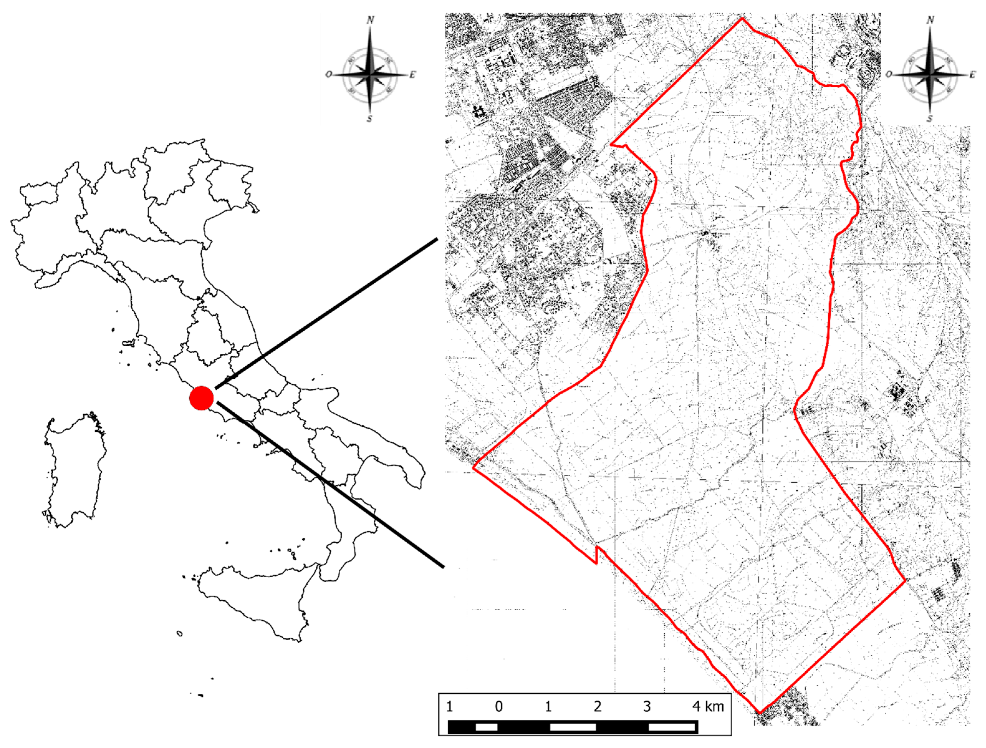
This study was carried out in the Presidential Estate of Castelporziano-Capocotta (Rome, Italy) (N 41°74′; E 12°40′) (
Figure 1). The Savoy Royal Family acquired it as a hunting reserve in 1872. In 1977, hunting was banned and it was instituted as a State Natural Reserve in 1999 [
28]. The forest has been managed by a policy of minimum-intervention and without removal of deadwood. About 4,578 ha of the Reserve are classified as woodlands, and it represents the most important Mediterranean lowland forest of Central Italy. Castelporziano is also in Rete Natura 2000, and the reserve area is a Special Protection Area (SPA). Moreover, there are two biotopes recognized as Community Interest Site (SCI): one for the coastline (IT6030027) and one for hygrophilous oak forests (IT6030028).
The Castelporziano estate conserves the last remaining part of the coastal environment, which was once all forest and the wet lowland of the Mediterranean area. Most of this estate is made up of a forest area, which is flat and characterized by deciduous oaks (
Quercus robur L.,
Q. frainetto Ten.,
Q. cerris L.), evergreen oaks (
Quercus ilex L.,
Q. suber L.), poplars, ash trees, alders, maples, and hornbeam [
29]. The umbrella pine (
Pinus pinea L.) was previously planted for fruit production and constitutes a characteristic element of the landscape [
30]. The cultivation activities for pine fruit are no longer practiced. The management of the forest aims to promote ecosystem conservation and natural regeneration.
The area is flat or gently rolling, which ranges in elevation between 0 to 80 m a.s.l. The hygrophilous lowland forest occupies most of the area. It is characterized by Mediterranean pines high forests, evergreen trees, and deciduous oak forest, and by more hygrophilous species near wet areas.
Average monthly temperatures range between a minimum of 8.4 and a maximum of 24.7 °C in the period of 1996–2011. The maximum values are generally reached in August and the minimum are reached in February without freezing events. The drought period starts in May and ends in early September. The average annual rainfall is 745 mm. Rainy events are more frequent in autumn with a low monthly rainfall during the May-August period [
31].
For this specific study, three different forest types were selected, characterized by pine, deciduous oak, and evergreen oak, typical of the Mediterranean lowlands. The forest types studied as a whole cover an area of almost 3000 ha in the Castelporziano estate. The three forest typologies investigated specifically have a total area of just over 200 ha. This selection was done on the basis of the actual forest management plan, choosing the most representative forest typologies not only of the Castelporziano estate, but also of managed Mediterranean lowland forests.
2.2. Data Collection
2.2.1. Sampling Design for Volume Estimation of Standing Live and Dead (snags) Trees and Stumps
For a systematic plot sampling a grid with dimension of 100 m × 100 m was used to locate sapling plots (every second grid centre) from north to south. These plots were for estimating the volume of standing live trees, snags, and stumps. Shape of sample plots was circular. The area of each sample plot was 706.5 m2 (r = 15 m) for pine type and 314 m2 (r = 10 m) for oak ones. Total sampling aimed to cover 3% of the three forest typologies and included 29 for pine sample plots, 60 for deciduous oak, and 60 for evergreen oak.
Although the state of coppice was still evident in the evergreen oak forest, the old stumps were not clearly recognizable.
The diameter at breast height (DBH ≥ 3 cm) of all living tree species was recorded to the nearest cm using a forest caliper. The tree height was estimated by the Haglof Vertex hypsometer and used to construct a hypsometric curve. The growing stock was determined by using local volume tables [
32]. For all snags sampled, species, DBH (DBH ≥ 3 cm), height, volume, and decay class (
Table 1) were recorded. Volume of snag, smaller than 4 m, was calculated using Huber’s formula.
2.2.2. Sampling Design for Volume Estimation of Downed Logs
One of the most efficient and accurate methods for estimating the volume of fallen wood, natural and logging residues, is the line intersect sampling method, which is widely used [
33,
34,
35,
36,
37]. Fifty meters of sampling line were located at the same grid centers of systematic sampling plots used for the dendrometric analysis. To reduce bias associated with piece orientation, each of the line transects was oriented on north-south and east-west resulting in four transect radiating for every plot centre. All fallen logs intersected by the line transects were measured. Only pieces at least 3 cm in diameter under bark and 30 cm in length were considered measurable. The measurement recorded for each piece of fallen wood was the diameter at the point of intersection with a transect line. The volume and weight of fallen wood in each line transect was computed by Equations (1) and (2), respectively [
38].
where
Vj is volume (m
3 ha
−1) in line transect j,
L is length of line transect (50 m),
dij is the diameter (cm) of piece
i in line transect j, n is number of pieces intersected in line transect
j,
Wj is weight (t/ha) in line transect j,
S is the specific gravity of pieces (g cm
−3). The number of pieces was computed by Equation (3) [
38].
where
Ni is the number of pieces per hectare in diameter class
i,
ni is number of tallied intersections in diameter class i,
L is the length of the sample line, and
di is the midpoint of the diameter class
i.
The volume of each piece (fallen log, stump, and snags with height lower than 4 m) was computed by the Huber formula, as shown in Equation (4) [
38,
39].
where
V is volume (cm
3),
dm is diameter under bark at the middle of the piece (cm), and l is length of piece (cm).
For each downed log, species and decay class were also recorded.
The botanical species of the CWD was assessed from the bark and macroscopic wood characteristics. Sometimes species were not reliably recognized and remained unspecified. Bark coverage was visually estimated.
2.2.3. Classification of Snags and Downed Logs in Decay Classes
Decay state of snags and logs [
12,
24,
40] was evaluated according to physical characteristics and bark coverage that was visually estimated by following the characters synthetised in
Table 1 [
24]. Each snag and log sampled was assigned to one of the five decay classes (DC).
2.2.4. Basic Density, Green Density, and Moisture Content of Decayed Samples
A total of 450 samples were collected covering three forest type (150 samples for each), two deadwood categories (225 samples for each), and five decay class (90 samples for each). Cylindrical samples of wood were collected using a drill with a cylindrical coring. Samples were carefully stored to avoid moisture loss. Analyses were carried out in a laboratory to determine mass, volume, green density, basic density, and moisture content. The green density of the wood was calculated on the samples in the fresh state as a ratio of mass to volume. The basic density was calculated as the ratio of dry mass to swollen volume. The volume of deadwood samples was determined by the volume of the cylindrical extractor. For splinted or irregular fresh samples, the volume was calculated with the water-displacement method [
41]. Fresh mass and dry was obtained with a laboratory precision balance. Dry mass was determined by a gravimetric method after drying to constant mass in an oven at a temperature of 103 °C ± 2 °C. The mass was considered constant when successive weighing, at intervals of at least 6 hours, showed the weight loss was no greater than 0.5% of sample mass.
2.3. Data Analysis
2.3.1. Carbon Stock Calculation
The carbon stock of deadwood was estimated by transforming deadwood volume into carbon mass. The basic density, which is obtained for each decay class, was used to convert the deadwood volume to mass. The carbon stock was estimated for each decay class. Specifically, different assessment coefficients were applied (49.0% according to Intergovernmental Panel on Climate Change (IPCC) [
42], 50.54% for pine, and 48.1% for oak, according to Thomas and Martin [
43]). The latter specific values were used to better focus on a Mediterranean context.
2.3.2. Deadwood Dynamic
The ratio of snag volume to stand volume (RSS) or snag creation index is a snag-dynamic indicator and it was calculated according to Equation (5).
The ratio of downed-log volume to volume of standing live trees (RDT) was also used as a downed-log creation index, according to Equation (6).
For comparing snag longevity, the ratio of downed-log volume to snag volume (RLS) was calculated according to Equation (7).
To evaluate past management legacy on CWD, the ratio of CWD volume to volume of standing live trees (RDW) was calculated, according to Equation (8).
where SGV is snag volume, LTV is the living tree volume, DLV is log volume, and DWV is the volume of the deadwood.
2.4. Statistical Analysis
Statistica 7.1 (2007, StatSoft Inc., Tulsa, OK, USA) software was used to implement statistical analyses. Field data were used for statistical surveys in order to validate results. Particularly, after checking for the normality variance (Lilliefors test) and homogeneity of variance (Levene’s test), parametric tests such as ANOVA groups, linear and no-linear regressions were used to compare the averages of stand variables and the linkages between factor (decay class (DC), forest type, growing stock) to each studied parameter (basic density, green density, and moisture content). The analysis of factorial variance (ANOVA tests) was carried out to relate the weight that each classification factor had on the parameters. In particular, the forest type and DC factors and their interaction were considered. Other factors (localization, altitude, growing stock) were investigated, but did not provide any valid evidence. Multiple comparisons were performed using a post-hoc Tukey test (HSD). The results of the analyses were also presented by using descriptive statistics.
3. Results
3.1. Growing Stock, Species Composition, and Diameter Distribution of Living Trees
The species composition in Pine forest is dominated by umbrella pine with more than 87% of living tree volume (
Table 2). In the Deciduous oak high forest (
Table 3), Turkey oak and peduncolate oak contribute to total stand volume more than 86% and in the evergreen oak forest (
Table 4), cork oak and holm oak contribution to growing stock is more than 50%.
Ancillary tree species were found to be associated with the main species. peduncolate oak, holm oak, and green olive (Phillyrea latifolia L.) were present elsewhere. Holm oak and laurel (Laurus nobilis L.) were more frequent in the pine forest, and sporadic, large deciduous oaks from the old forest were found, preserved in the umbrella pine plantation. In the deciduous oak stand, hornbean (Carpinus orientalis Mill.) was found with holm oak and tree heat (Erica arborea L.). Pine and deciduous oaks were also associated with the species of Mediterranean maquis. A greater richness of tree species was observed in the evergreen oak forest.
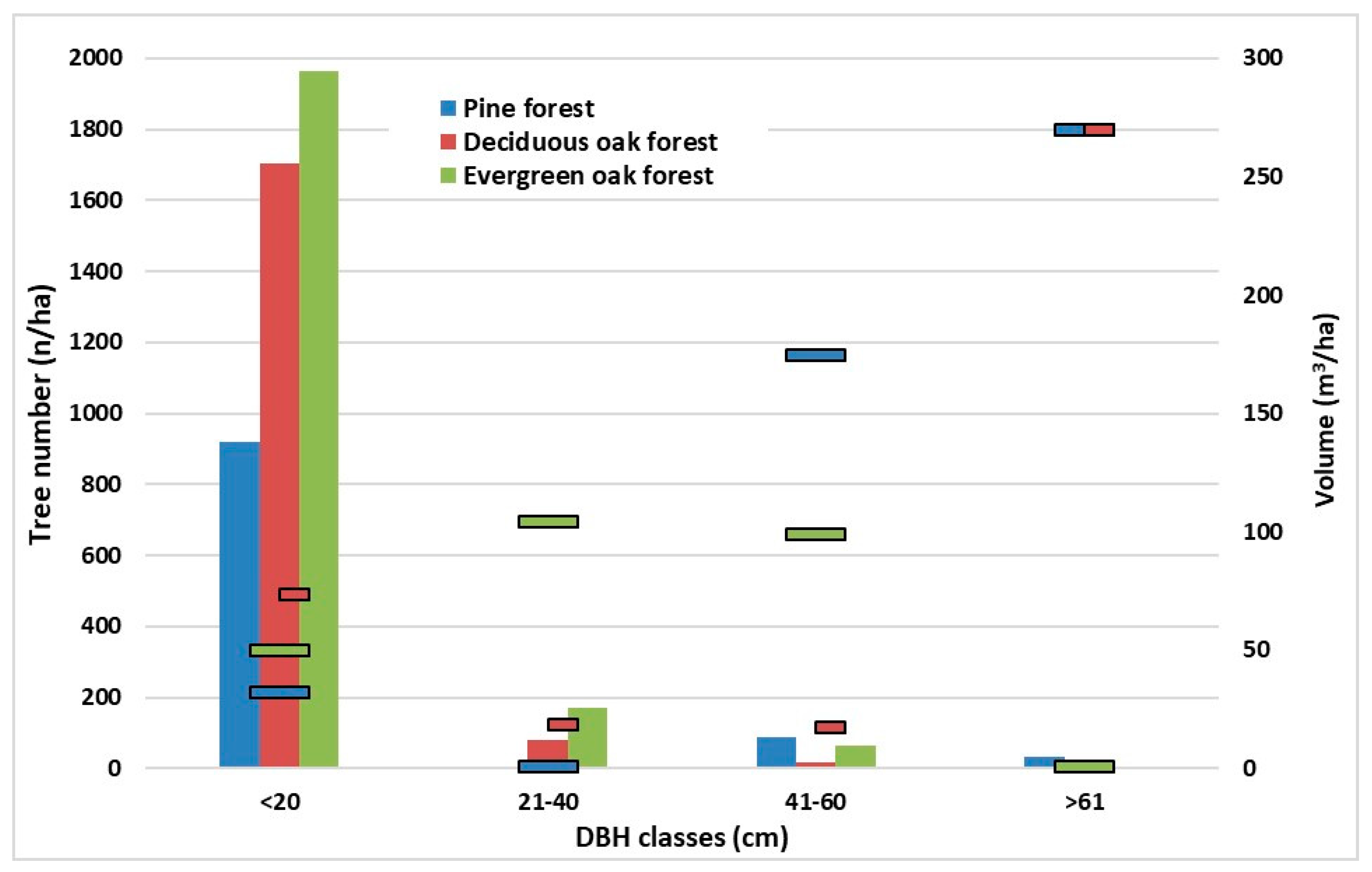
The largest number of living trees was noticed in the lower diameter class in each examined forest type (
Figure 2). The larger diameter class had the higher tree volume, coupled with the least number of trees, in pine and deciduous oak type (
Figure 2). No trees >61 cm in diameter were found in the evergreen oak forest probably due to the coppiced origin. In fact, 11% of the trees stocking, which comprised 80% of the growing stock volume, were represented in 21–60 cm diameter classes (
Figure 2).
3.2. Deadwood Volume by Component, Species, Diameter Classes, and Decay Class
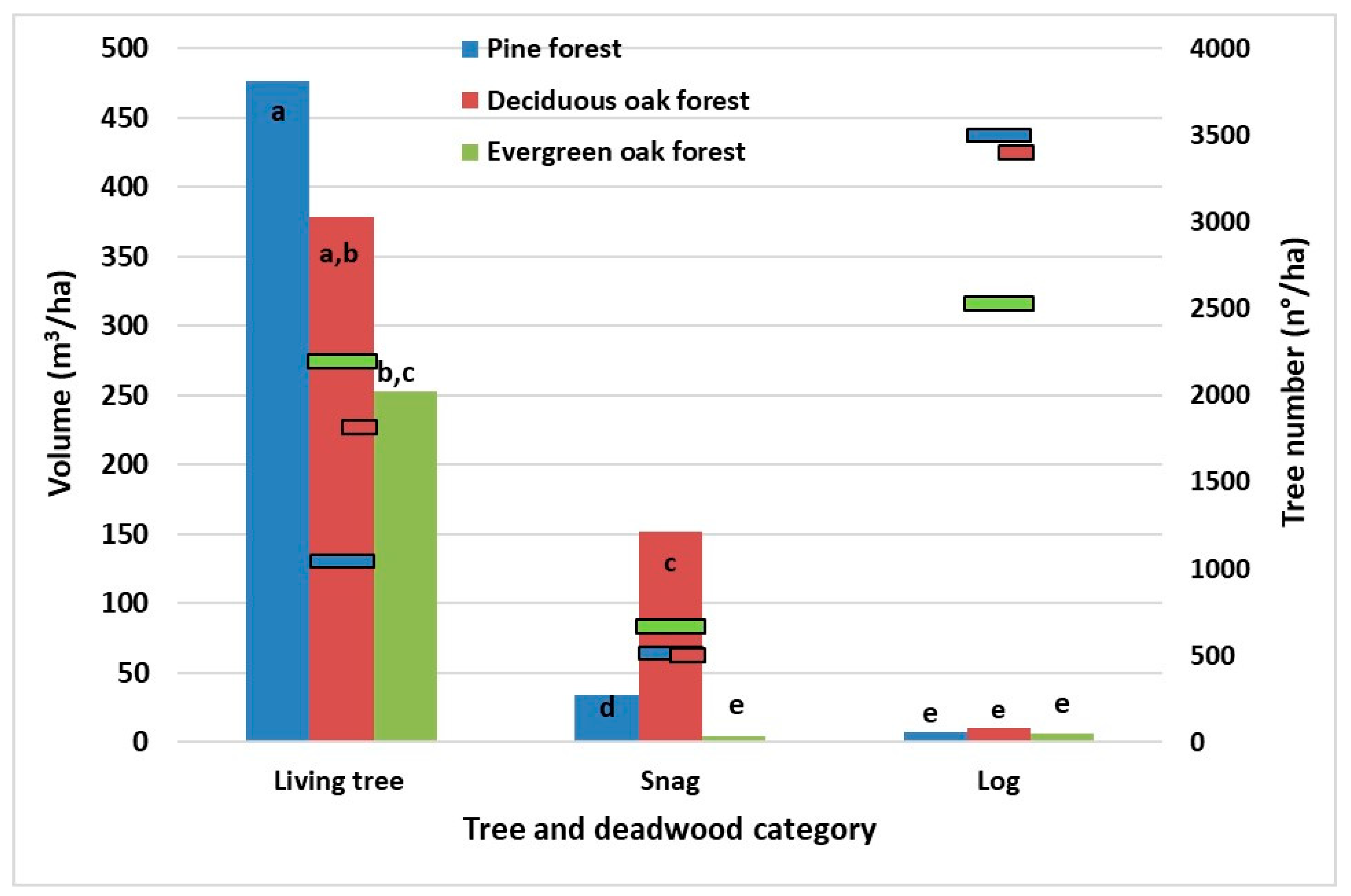
The quantities of living trees and deadwood were largely different (
Figure 3), according to the prevailing species and past management of the different stands. ANOVA test showed statistically significant differences and the HSD post hoc test detected five homogeneous groups (
Figure 3). The living tree volume of the pine forest was statistically different.
In the pine forest, composed of great umbrella pines, some large oak snags of the old original forest were detected; the volume of snags accounts for 82% of the total volume of deadwood. The highest volume amount of deadwood was found in mixed deciduous oaks high forest (161.85 m
3/ha). It was mainly composed by oak “habitat trees” or snags. The snags prevailed in deciduous oak forest (62%) by volume. The lower amount of deadwood was found in evergreen oak forest (11.0 m
3/ha). The volume of snags and logs was similar. The log category showed no statistical difference in volume as the HSD post hoc test highlighted (
Figure 3).
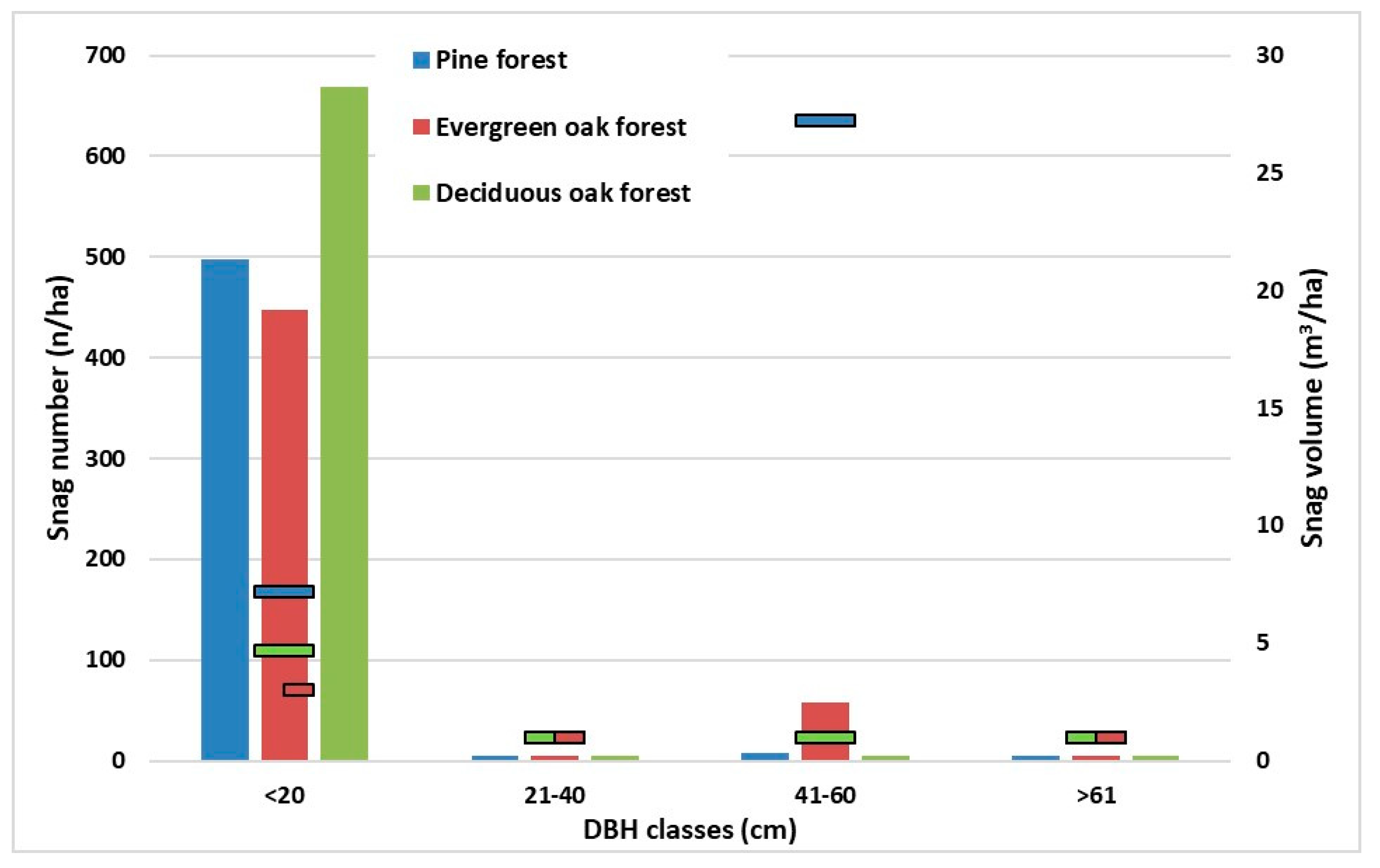
Figure 4 describes the snag distribution by number and volume in each forest type. Snag species mirrored the stand composition in oak types in general (data not shown). Nevertheless, no pine was detected as snag in the pine forest. Green olive and laurel were the common snag species in each type, with snags of deciduous oak, identified only to a genus level. The volume of snags of cork oak was the highest, as was the volume of the living trees in the evergreen oak forest. The species with the highest snag frequency by number was the hornbeam in the deciduous oak type and the volume of oak was high.
Figure 5 describes the log distribution by number and volume in each stand. Sometimes, it was not possible to recognize the log species using macroscopic anatomical features or bark characteristics (data not shown), so some remained unattributed. In the pine forest, the logs were almost all branches of umbrella pine and they were associated to the lower DBH class (
Figure 5). In deciduous oak forest, the main contribution both in number and volume came from peduncolate oak, falling in the lower DBH class. In the evergreen oak forest, log species was mainly non-attributed. 97% was in the lower DBH class, representing 44% by volume.
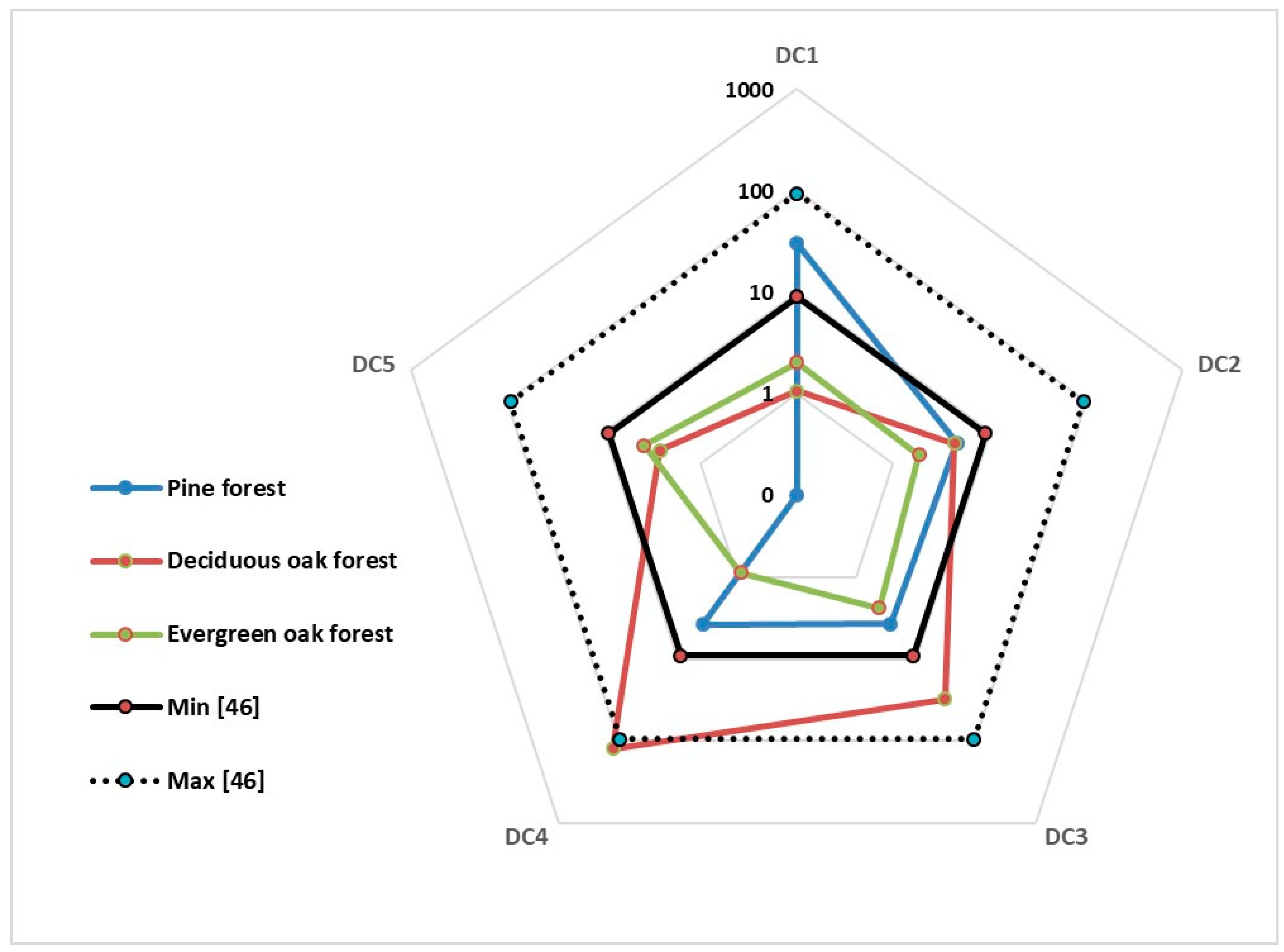
The distribution in the decay classes (DC) of logs and snags was shown in
Figure 6 and
Table 5. In all the examined stands, the snags in DC 1 still preserved the physiognomy of trees. The DC 1 had the most numerous and the largest volume of snags in the pine type and in the evergreen coppiced oak type. The ore degraded classes had the lower values. The pine type showed no snags in DC 5. In the deciduous oak type, DC 4 snags reached the highest volume of both classes and forest type (123.24 m
3/ha). Logs were absent in the first and last DC of the pine type. In the deciduous oak type, the most represented decay class was DC 2. It is worth remembering that logs were only in the first diameter class (<20) in pine and deciduous oak types and that the diameter class 21–40 had 44% of the log volume in the evergreen oak type.
3.3. Deadwood Dynamic
In
Table 6, the deadwood dynamic indices were presented. A higher RSS value was found in the deciduous oak forest type compared to the pine (7.23%) and evergreen oak coppiced (1.86%) types, likely due to a lower volume of snags in these areas. The RDW showed a similar behavior, probably due to the higher amount of deadwood in deciduous oak forest driven by snag volume. Similarly, a log creation index (RDT) was higher in the deciduous oak forest. The RDT value was influenced by snag longevity and reflected the log dynamics in the analyzed stands. In fact, RLS was lower in the deciduous oak forest and higher in the evergreen oak coppiced forest.
3.4. Analysis of Decayed Samples and Carbon Calculation
3.4.1. Basic Density, Green Density, and Moisture Content ANOVA Test
The ANOVA factorial test was applied to test the possible influence of stand typology, wood decay class and their mutual interaction for the variables: basic density, green wood density, and wood moisture. Statistically significant difference was highlighted for basic density only within decay classes (p = 0.032) (data not shown), while for the forest types the p-value was >0.05 (p = 0.46). There was no statistical differentiation in the interaction between these two factors (p > 0.05). Similar results were obtained for green density. Statistically significant difference was found for decay classes (p < 0.041) (data not shown), but forest type (p = 0.38) and the interaction between the factors were not statistically significant (p > 0.05). Likewise, there were no significant differences (p > 0.05) for the wood moisture content.
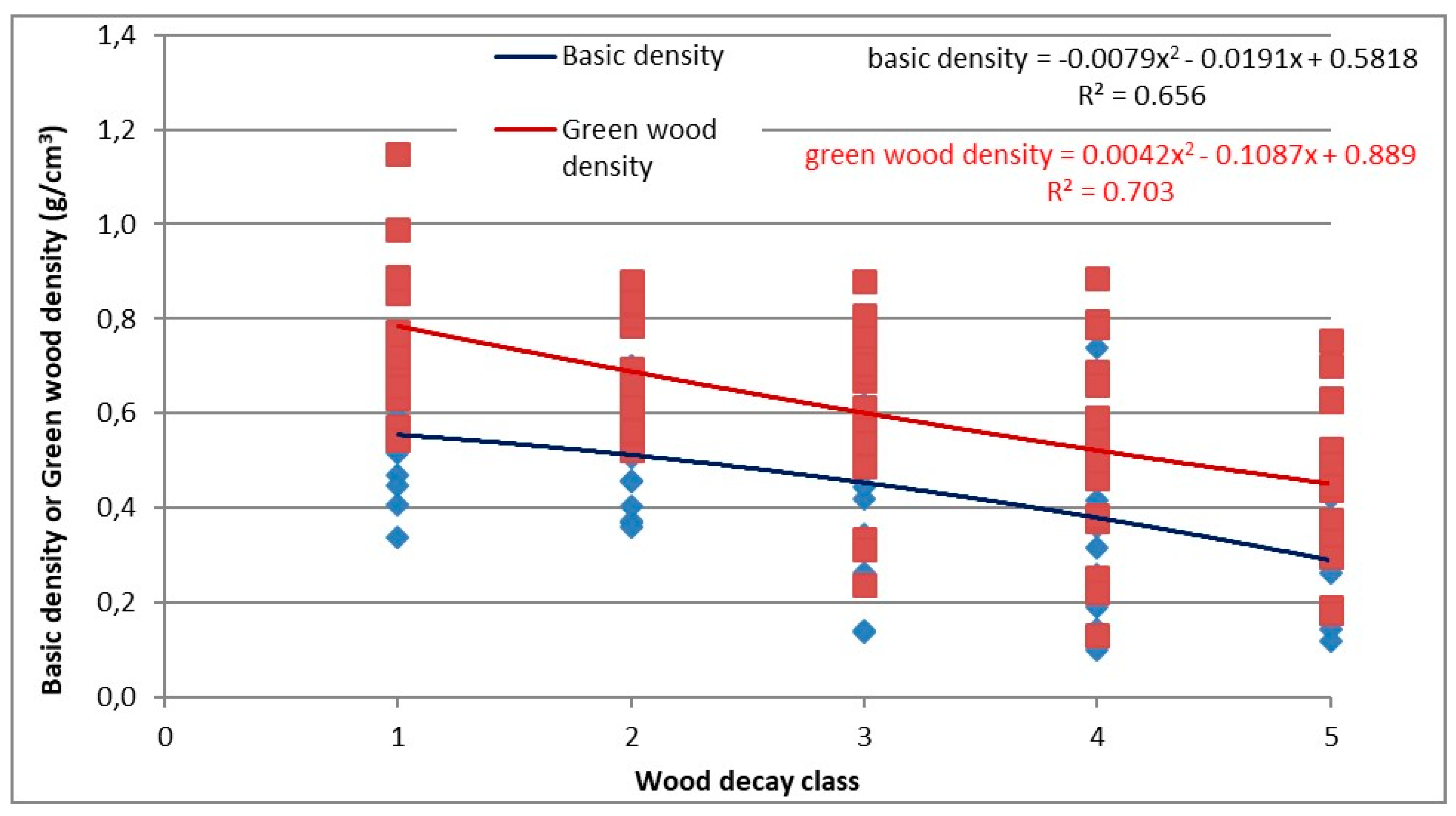
3.4.2. Basic Density and Green Density
Considering the results of the ANOVA factorial test on basic density and green density, a non-linear regression analysis was conducted. These analyses excluded the forest type parameter as statistically significant. The decay class was the only significant independent variable for both basic density and green wood density. The value of the regression coefficient for basic density was R
adj2 = 0.656, and, for green wood density, was R
adj2 = 0.703, the overall regression was statistically significant. The polynomial curves are shown in
Figure 7.
3.4.3. Carbon Stock
According to
Table 7, the C-stock in deadwood in the pine type was estimated to be 10.84, which follows the Intergovernmental Panel on Climate Change (IPCC) indication [
42], or 11.18 t ha
−1, as more accurately for the Mediterranean context [
43]. The DC 1 contributed the most (75%). In deciduous oak type (
Table 8), the C-stock was estimated respectively 31.43 and 30.85 t ha
−1. DC 4 mostly contributed (73%), DC 3 contributed with about 22%. The lowest contribution was in DC 1, lower than 1%. In the evergreen oak type (
Table 9), the C-stock was estimated to be, respectively, 2.26 and 2.21 t ha
−1. DC 1 and DC 5 equally contributed about 25%; DC 3 had a lower but similar contribution (24%).
4. Discussion
4.1. Growing Stock, Species Composition, and Diameter Distribution of Living Trees
This pine forest, which is dominated by large umbrella pine trees, was planted in the last century for fruit production. It is considered to be an element of cultural landscape [
30]. The management decision to reduce silvicultural interventions to exclusive phytosanitary surveillance has produced the effect of amplifying the presence of auxiliary species both in terms of quantity and richness. At the beginning of this century, the low anthropogenic disturbance had allowed holm oak and green olive to invade the forest [
45]. The decision to preserve the great trees of the previous cycle and not to remove the few senescent or dead trees of large size contributed to make the Castelporziano estate different from the surrounding forests and from those of Central and Southern Italy, managed for timber production. It is also unique for the considerable extent of the forest area. The large deciduous oaks from the old forest were few, but largely contribute to the volume stock of the ancillary species in pine forest. The large deciduous oaks, still alive, showed some large branches in decline that can contribute to an increase in the downed log component in the future. The forests of deciduous oak and umbrella pine showed fewer other species of trees than the evergreen stand probably due to previous management. In theory, the decision to stop the coppicing practice could favour the closure of the crown layer, basically constituted by the standards and best-developed sprouts and induced strong competition between the shoots of the dominated biospace.
4.2. Deadwood Volume by Component, Species, Diameter Classes, and Decay Class
In this Mediterranean area, the possibility of a continuous accumulation of deadwood over time is usually a result of the natural disturbance and the abandonment of the timber harvest [
7,
46,
47,
48,
49,
50,
51] or, better, of the choice to carry out minimal interventions since the removal of deadwood has been one of the most frequent operations in forest, favoured by the rights of use of local populations for the collection of deadwood as firewood [
15,
24,
25] and the fear of forest fires by managers. Deadwood is mainly caused by tree mortality and the accumulation is due to the production coupled with the degradation and decay of biological agents [
6,
52,
53,
54].
Deadwood in deciduous oak type amounts to 4 times that of pine and almost 15 times that of the evergreen oak type. The pine type and the deciduous oak type differed from the evergreen oak type due to the higher growing stock and the quantity of deadwood. The proportion of deadwood component types (snags and logs) varies with the past management approach. As found also by other authors [
55,
56], deadwood amount and its components depended significantly on forest type, age from the reserve establishment and volume of living wood. The time elapsed since the last harvest was noted as a factor influencing deadwood accumulation, which is particularly evident in aged coppice [
7,
46].
Most snags belonged to the smallest diameter class in each forest type. These were dead standing trees that had occupied a less favourable biospace. Competition between neighbouring trees is the most frequent cause of mortality [
57]. It was observed that the structural evolution in the aged stand is still ongoing, markedly in the evergreen oaks coppice of the study area. Banaś et al. [
58] observed that small size trees mostly die while standing, medium-sized trees have the greatest chance of survival, and very large trees experience increased mortality rates, mainly due to uprooting or breakage.
The diameter distribution of the snags combined with the decay stage provided further information. The aging of coppice led to the death of smaller and less competitive trees [
7,
46,
47]. The decay stage, DC 1, indicated recent death.
A great contribution for the accumulation of deadwood on the ground was in the form of branches or logs landed as a result of natural disturbances in adult stands or as residues of forest loggings [
59,
60]. This behaviour was observed on the pine type, as the downed logs mainly belonged to pine branches, broken by natural events. The contribution of downed logs to the volume of deadwood was low in the types of pine and deciduous oaks, but more than 50% in the evergreen oak type due to the breaking of the standards, probably related to the competition between neighbours [
48].
In the short-term future, deadwood amount can be expected to increase by the mortality due to endogenous processes, such as competition, senescence, and natural disturbances, coupled with low anthropic intervention [
49,
55,
61]. However, deadwood could be removed to reduce the hazard of wildfire and pests [
61] due to the vicinity of a densely populated city like Rome.
The quality, amount, and decay classes of deadwood can provide information on mortality processes and disturbance occurrence [
62,
63,
64]. The large amount of DC 1 due only to snags was related to the suppression of the broadleaf species in the pine forest. The broken branches of pine, even of great diameter, early decayed on the forest ground, due to the low natural durability of this wood. Moreover, selective cutting over time on pine trees for phytosanitary or safety purposes may have also reduced the amount of deadwood and, consequently, have decreased the amount of CWD in the higher decay classes [
9,
50].
In the deciduous oak forest, the high amount of deadwood in DC 3 and DC 4 was caused by the snags of large old oak trees from the previous cycles and their higher wood durability. Despite the low amount of deadwood in DC 5, most are logs [
48]. More than the other cases studied, the current silvicultural choices have a fundamental impact on the dynamics of deadwood accumulation of the future as well.
As observed by Badalamenti et al. [
44] in similar conditions, the amount of CWD in the evergreen oak forest was more equally distributed between categories in each decay class and, conversely, the snags prevailed in DC 1 and DC 2. In the other cases, log frequency was higher and consisted of woody debris that had naturally fallen and never been removed.
4.3. Deadwood Dynamic
The higher amount of CWD was conditioned by the biomass of living trees [
49,
65]. In the study area, the stand volume differences were also associated with differences in the accumulation of CWD, which was also conditioned by previous management choices. The effects of past management were particularly evident in the deciduous oak forest by considering each dynamic index examined.
The snag creation index (RSS) generally was higher in unmanaged or in low human pressure forest, as previously reported [
4,
24].
Log creation index (RDT) showed a low rate at each forest type, although the deciduous oak forest had the highest value. It indicated that the structuring of the CWD was still in its initial phase. RDT progressively increase as time elapses from management abandonment. Downed deadwood turns prevalent in other mesic oak stands [
47,
51,
52].
The snag longevity index (RLS) was influenced by snag degradation and decay and reflects the log dynamics in the analyzed compartments. A higher RLS value was associated with managed forests [
4]. A great number of snags preserved the height of the tree and had not yet undergone natural breakage. The values of RLS were higher than 1 in all forest type. The lower management pressure in the recent years on the evergreen oak and pine forest was reflected by the RDW lower value for the deciduous oak type, and the RLS value, which was 20 and 3 times, respectively, higher than the deciduous oak forest. Also, the value of the snag longevity index (RLS) depends on the ecological factors such as tree species composition, wind speed, snow accumulation, ground slope, stand canopy closure, stand density, number of story layers (vertical layers and structure), stand age, and stand successional stage. The lower snag creation index (RSS) was caused by the higher snag longevity index (RLS) in the evergreen oak forest, as found by Moorman et al. [
66].
4.4. Analysis of Decayed Samples and C Calculation
Deadwood represents a fraction of the carbon stored in forests [
20,
21]. In forests with low management intensity or in reserve areas, this ecosystem component is considered essential not only for the aspects strictly connected to biodiversity but also for the carbon content slowly released into the environment due to wood degradation and decay. Matsuzaki et al. [
21] found that live trees, snags, CWD, and forest floor accounted for 76%, 5%, 9%, and 10% of the total forest C stocks, respectively. In this study, the pine forest type, accounted for 81%, 7%, 1%, and 11% of the total forest C-stocks in the same respective categories; the deciduous oak forest for 70%, 19%, 1%, and 10%; and the evergreen oak forest for 86%, 1%, 1%, and 12% of the total forest C-stocks. In this context, basic densities’ accuracy to estimate forest deadwood biomass was necessary to obtain reliable value [
67]. Our results indicated clearly that the only factor affecting green density and basic density was decay class. Carbon content reflected the decay state and depended on the volume of deadwood in each forest type. In the pine and deciduous oak forest, only one decay class prevailed. The evergreen oak forest type showed a more homogeneous distribution in each decay class and the lower amount of deadwood and C-stock, probably due to the relatively recent choices of minimal crop intervention, which induced tree mortality by competition.
The different ways to calculate the carbon content had shown similar results in this context, but more accurate methods that consider the differences between coniferous and angiosperm wood are preferable, especially in mixed contexts [
43].
Total dead wood accounted for an assessed range of 2% to 20% of total aboveground C storage (2% evergreen oak forest, 20% deciduous oak forest, and 8% oak forest). These values reflect other studies [
68,
69,
70,
71,
72] with a large range of variation from less than 2% to more than 40%.
5. Conclusions
The research protocol was designed to better understand the amount and the dynamics of deadwood in protected areas with the aim to provide a valuable baseline for sustainable management in actively managed stands in Mediterranean forests as well.
The following four conclusion are drawn:
1. The major component of deadwood was the standing dead trees or snags. There was a higher volume of deadwood in the deciduous oak forest than in the pine and evergreen oak forest.
This first finding highlighted some aspects related to the vulnerability of the deciduous oak forest in the Mediterranean climate. For this reason, managers should pay particular attention to forest management in specific wild or natural areas.
2. The amount of deadwood was affected by the forest type and forest management regime. Dynamic and past management of deadwood indices indicated that their structure was still in an initial phase of creation and decay class in the pine and evergreen oak forests.
This finding highlighted a slower creation and evolution of deadwood in pine compared to aged evergreen oak forests. By contrast, dynamic processes were much more pronounced in the deciduous oak forest. For these reasons, forest management should seek to prevent fire risks.
3. The carbon stored in deadwood ranged from 10.84 to 11.18 t ha−1 in the pine forest and most of the deadwood was found in DC1 (75%). In the deciduous oak stand, the C-stock ranged from 30.85 to 31.43 t ha−1 and the majority was classified as DC 4 (73%). In the evergreen oak forest, the C-stock ranged from 2.21 to 2.26 t ha−1 and with equal quantities in both DC 1 and DC 5 about 25%.
The situation of the pine forest in relation to the longevity of the carbon in the deadwood pool could be considered the most positive one (mainly in DC1), in comparison to the other two forest types, where the deadwood was mainly in DC4 and DC5. Active management of deadwood pool to maintain a high percentage of deadwood in DC1 will assure a gradual passage to the other decay classes. This aspect is important for lengthening carbon storage as well as other ecological implications.
4. In the Mediterranean lowland forests, as found in this study, deadwood could play a distinct role in carbon storage, but, generally a marginal one (2–9%). Depending on past management or pest/diseases activities (deciduous oak forest), this value could be near 20% but could possibly increase beyond 40%.
This finding for these three Mediterranean forest types indicates a high variability of carbon storage within the deadwood component. For this reason, the calculation methodology is of vital importance. The basic density of each decay class improved accuracy in assessing the carbon stock in deadwood. Lengthening the period of carbon storage implies maintaining large quantity of deadwood in DC1, as this material has the higher basic density.
In summary, species composition, growing stock, and deadwood features indicated that the legacy of past management still heavily influenced the physiognomy of these stands. A major component of deadwood was the standing dead trees or snags. The driving factors that determine the amount of coarse woody debris and snags range from low management intensity to abandonment. These cause mortality by competition. Therefore, the qualitative and quantitative characteristics of the deadwood indicated that the structuring of the CWD is still in its initial phase.
Author Contributions
Conceptualization, A.L.M. and R.P. Methodology, A.L.M. and R.P. Validation, A.L.M. and R.P. Formal analysis, A.L.M., F.T., and R.P. Investigation, A.L.M., G.L., F.L., and R.P. Data curation, A.L.M., G.L., F.L., F.T., and R.P. Writing—original draft preparation, A.L.M., G.L., and F.L. Writing—review and editing, A.L.M. and R.P. Visualization, A.L.M., F.L., F.T., and R.P. Supervision, A.L.M. All authors have read and agreed to the published version of the manuscript.
Funding
This research did not receive any specific grant from funding agencies in the public, commercial, or not-for-profit sectors.
Acknowledgments
The authors are grateful to the Segretariato Generale delle Presidenza della Repubblica, Tenuta di Castelporziano, for allowing the investigations. This research was in part carried out within the framework of the MIUR (Italian Ministry for Education, University and Research) initiative “Departments of Excellence” (Law 232/2016), WP3 (R. Picchio) and WP 4 (A. Lo Monaco), which financed the Department of Agriculture and Forest Science at the University of Tuscia.
Conflicts of Interest
The authors declare no conflict of interest.
References
- FAO Global Forest Resources Assessment 2005. Progress Towards Sustainable Forest Managent. Available online: http://www.fao.org/3/a0400e/a0400e00.htm (accessed on 26 February 2020).
- Gasparini, P.; Tabacchi, G. L’inventario Nazionale delle Foreste e dei Serbatoi Forestali di Carbonio INFC 2005. Secondo Inventario Forestale Nazionale Italiano; Ministero delle Politiche Agricole, Alimentari e Forestali; Corpo Forestale dello Stato; Consiglio per la Ricerca e la Sperimentazione in Agricoltura, Unità di ricerca per il Monitoraggio e la Pianificazione Forestale; Edagricole-Il Sole 24 ore: Bologna, Italy, 2011. [Google Scholar]
- Tavankar, F.; Bonyad, A.E.; Iranparast Bodaghi, A. Effects of snags on the species diversity and frequency of tree natural regeneration in natural forest ecosystems of Guilan. Iran J. Plant Res. 2013, 26, 267–280. [Google Scholar]
- Tavankar, F.; Nikooy, M.; Picchio, R.; Venanzi, R.; Lo Monaco, A. Long-term effects of single-tree selection cutting management on coarse woody debris in natural mixed beech stands in the Caspian forest (Iran). iForest 2017, 10, 652–658. [Google Scholar] [CrossRef] [Green Version]
- Harper, K.A.; Bergeron, Y.; Drapeau, P.; Gauthier, S.; De Grandpré, L. Structural development following fire in black spruce boreal forest. For. Ecol. Manag. 2005, 206, 293–306. [Google Scholar] [CrossRef]
- Pedlar, J.H.; Pearce, J.L.; Venier, L.A.; McKenney, D.W. Coarse woody debris in relation to disturbance and forest type in boreal Canada. For. Ecol. Manag. 2002, 158, 189–194. [Google Scholar] [CrossRef]
- La Fauci, A.; Mercurio, R. Caratterizzazione della necromassa in cedui di castagno (Castanea sativa Mill.) nel Parco nazionale dell’Aspromonte. Forest 2008, 5, 92–99. [Google Scholar] [CrossRef] [Green Version]
- Vallejo, V.R.; Arianoutsou, M.; Moreira, F. Chapter 5 Fire Ecology and Post-Fire Restoration Approaches in Southern European Forest Types. Post-Fire Management and Restoration of Southern European Forests; Managing Forest Ecosystems; Springer: Dordrecht, The Netherlands, 2012. [Google Scholar]
- Ganteaume, A.; Camia, A.; Jappiot, M.; San-Miguel-Ayanz, J.; Long-Fournel, M.; Lampin, C.A. Review of the Main Driving Factors of Forest Fire Ignition Over Europe. Environ. Manag. 2013, 51, 651–662. [Google Scholar] [CrossRef] [PubMed] [Green Version]
- Picchio, R.; Spina, R.; Calienno, L.; Venanzi, R.; Lo Monaco, A. Forest operations for implementing silvicultural treatments for multiple purposes. Ital. J. Agron. 2016, 11, 156–161. [Google Scholar]
- Bertolotto, P.; Calienno, L.; Conforti, M.; D’Andrea, E.; Lo Monaco, A.; Magnani, E.; Marinšek, A.; Micali, M.; Picchio, R.; Sicuriello, F.; et al. Assessing indicators of forest ecosystem health. Ann. Silv. Res. 2016, 40, 64–69. [Google Scholar]
- Corace, R.G.; Seefelt, N.E.; Goebel, P.C.; Shaw, H.L. Snag longevity and decay class development in a recent jack pine clear-cut in Michigan. North. J. Appl. For. 2010, 27, 125–131. [Google Scholar] [CrossRef] [Green Version]
- Hanberry, B.B.; Hanberry, P.; Demarais, S.; Jones, J.C. Importance of residual trees to birds in regenerating pine plantations. iForest 2012, 5, 108–112. [Google Scholar] [CrossRef] [Green Version]
- Russell, R.E.; Saab, V.A.; Dudley, J.G.; Rotella, J.J. Snag longevity in relation to wildfire and post fire salvage logging. For. Ecol. Manag. 2006, 232, 179–187. [Google Scholar] [CrossRef]
- Wisdom, M.J.; Bate, L.J. Snag density varies with intensity of timber harvest and human access. For. Ecol. Manag. 2008, 255, 2085–2093. [Google Scholar] [CrossRef]
- Larrieu, L.; Cabannettes, A. Species, live status, and diameter are important tree features for diversity and abundance of tree microhabitats in subnatural montane beech-fir forests. Can. J. For. Res. 2012, 42, 1433–1445. [Google Scholar] [CrossRef]
- Nascimbene, J.; Thor, G.; Nimis, P.L. Effects of forest management on epiphytic lichens in temperate deciduous forests of Europe—A review. For. Ecol. Manag. 2013, 298, 27–38. [Google Scholar] [CrossRef]
- Mason, F.; Zapponi, L. The forest biodiversity artery: Towards forest management for saproxylic conservation. iForest 2015, 9, 205–216. [Google Scholar] [CrossRef] [Green Version]
- Hagan, J.M.; Grove, S.L. Coarse woody debris. J. Forest. 1999, 1, 6–11. [Google Scholar]
- Allard, J.; Park, A. Woody debris volumes and carbon accumulation differ across a chronosequence of boreal red pine and jack pine stands. Can. J. For. Res. 2013, 43, 768–775. [Google Scholar] [CrossRef]
- Matsuzaki, E.; Sanborn, P.; Fredeen, A.L.; Shaw, C.H.; Hawkins, C. Carbon stocks in managed and unmanaged old-growth western red cedar and western hemlock stands of Canada’s inland temperate rainforests. For. Ecol. Manag. 2013, 297, 108–119. [Google Scholar] [CrossRef]
- Morelli, S.; Paletto, A.; Tosi, V. Il legno morto dei boschi: Indagine sulla densità basale del legno di alcune specie del Trentino. Forest@ 2007, 4, 395–406. [Google Scholar] [CrossRef] [Green Version]
- Tavankar, F.; Picchio, R.; Lo Monaco, A.; Bonyad, A.E. Forest management and snag characteristics in Northern Iran lowland forests. J. For. Sci. 2014, 60, 431–441. [Google Scholar] [CrossRef] [Green Version]
- Behjou, F.K.; Lo Monaco, A.; Tavankar, F.; Venanzi, R.; Nikooy, M.; Picchio, R. Coarse woody debris variability as result of human accessibility to forest. Forests 2018, 9, 509. [Google Scholar] [CrossRef] [Green Version]
- Bate, L.J.; Wisdom, M.J.; Wales, B.C. Snag densities in relation to human access and associated management factors in forests of northeastern Oregon. Landsc. Urban Plan. 2007, 80, 278–291. [Google Scholar] [CrossRef]
- Perry, R.W.; Thill, R.E. Comparison of snag densities among regeneration treatments in mixed pine hardwood forests. Can. J. For. Res. 2013, 43, 619–626. [Google Scholar] [CrossRef]
- De Long, S.C.; Sutherland, G.D.; Daniels, L.D.; Heemskerk, B.H.; Storaunet, K.O. Temporal dynamics of snags and development of snag habitats in wet spruce-fir stands in east-central British Columbia. For. Ecol. Manag. 2008, 255, 3613–3620. [Google Scholar] [CrossRef]
- Pratesi, F. Castelporziano: History of a forest. Rend. Fis. Acc. Lincei. 2015, 26, S305–S310. [Google Scholar] [CrossRef]
- Pignatti, S.; Bianco, P.M.; Tescarollo, P.; Scarascia-Mugnozza, G.T. La Vegetazione della Tenuta Presidenziale di Castelporziano; Accademia Nazionale delle Scienze: Roma, Italy, 2001. [Google Scholar]
- Capitoni, B.; Giordano, E.; Maffei, L.; Recanatesi, F.; Scarascia-Mugnozza, G.T.; Tinelli, A.; Troiani, L. Problemi di rinnovazione delle pinete di carattere estetico e paesaggistico nella tenuta di Castelporziano. In Proceedings of the Atti del Terzo Congresso Nazionale di Selvicoltura per il miglioramento e la conservazione dei boschi italiani, Taormina, Italy, 16–19 October 2008. [Google Scholar]
- Fusaro, L.; Salvatori, E.; Mereu, S.; Silli, V.; Bernardini, A.; Tinelli, A.; Manes, F. Researches in Castelporziano test site: Ecophysiological studies on Mediterranean vegetation in a changing environment. Rend. Fis. Acc. Lincei. 2015, 26, 473–481. [Google Scholar] [CrossRef]
- Castellani, C. Tavole Stereometriche ed Alsometriche Costruite per i Boschi Italiani; Istituto Sperimentale per l’Assestamento Forestale e per l’Alpicoltura Publishing: Trento, Italy, 1970. [Google Scholar]
- Howard, J.O.; Setzer, T.S. Logging Residue in Southeast Alaska; USDA Forest Service, Agriculture, Forest Service, Pacific Northwest Research Station Publishing: Portland, OR, USA, 1989.
- Marshall, P.L.; Davis, G.; Taylor, S.W. Using Line Intersect Sampling for Coarse Woody Debris: Practitioners’ Questions Addressed; BC. Research Section, Coast Forest Region, BC Ministry of Forests: Nanaimo, BC, Canada, 2003.
- Lutes, D.C. Assessment of the line transect method: An examination of the spatial patterns of down and standing dead wood. In Proceedings of the Symposium on the Ecology and Management of Dead Wood in Western Forests; 1999 November 2-4; Reno, NV. Gen. Tech. Rep. PSW-GTR-181; Forest Service, Pacific Southwest Research Station: Albany, CA, USA, 2002; pp. 665–675. [Google Scholar]
- Tavankar, F.; Bonyad, A. Assessment of logging residuals from single selection cutting by Line Intersect method (Case Study: Parcel 237 from district 2 Asalem-Nav forest). J. Wood For. Sci. Techn. 2013, 20, 95–109. (In Persian) [Google Scholar]
- Tavankar, F.; Eynollahi, Y. Amount and characteristics of logging residues in selection cutting stand in the Northern forests of Iran. Int. J. Biosci. 2013, 3, 35–42. [Google Scholar]
- Van Wagner, C.E. Canada Information Report PI-X-12: Practical Aspects of the Line Intersect Method; Petawawa Canadian National Forestry Institute Forestry Service: Chalk River, ON, Canada, 1982.
- Waddell, K.L. Sampling coarse woody debris for multiple attributes in extensive resource inventories. Ecol. Indicator. 2002, 1, 139–153. [Google Scholar] [CrossRef]
- Hunter, M.L. Wildlife; Forests and Forestry; Prentice Hall: Englewood Cliffs, NJ, USA, 1990; p. 370. [Google Scholar]
- Lo Monaco, A.; Todaro, L.; Sarlatto, M.; Spina, R.; Calienno, L.; Picchio, R. Effect of moisture on physical parameters of timber from Turkey oak (Quercus cerris L.) coppice in Central Italy. For. Stud. China 2011, 13, 276–284. [Google Scholar] [CrossRef]
- Intergovernmental Panel on Climate Change (IPCC). Forest lands. In Intergovernmental Panel on Climate Change Guidelines for National Greenhouse Gas Inventories; Institute for Global Environmental Strategies: Hayama, Japan, 2006; p. 483. [Google Scholar]
- Thomas, S.C.; Martin, A.R. Carbon content of tree tissues: A synthesis. Forests 2013, 3, 332–352. [Google Scholar] [CrossRef] [Green Version]
- Badalamenti, E.; La Mantia, T.; La Mantia, G.; Cairone, A.; La Mela Veca, D.S. Living and Dead Aboveground Biomass in Mediterranean Forests: Evidence of Old-Growth Traits in a Quercus pubescens Willd. s.l. Stand. Forests 2017, 8, 187. [Google Scholar] [CrossRef] [Green Version]
- Della Rocca, B.A.; Pignatti, S.; Mugnoli, S.; Bianco, P.M. La Carta della Vegetazione della Tenuta di Castelporziano. In Il Sistema Ambientale Della Tenuta Presidenziale di Castelporziano; Scritti e Documenti XXVI; Accademia Nazionale delle Scienze: Roma, Italy, 2001; pp. 709–747. (In Italian) [Google Scholar]
- Marziliano, P.A. Analisi quali-quantitativa della necromassa in cedui invecchiati di leccio (Quercus ilex L.) del Gargano. Forest@ 2009, 6, 19–28. [Google Scholar] [CrossRef]
- Bertini, G.; Fabbio, G.; Piovosi, M.; Calderisi, M. Tree biomass and deadwood density into aged holm oak (Sardinia) and beech coppices (Tuscany). Forest@ 2012, 9, 108–129. [Google Scholar] [CrossRef]
- Paletto, A.; De Meo, I.; Cantiani, P.; Ferretti, F. Effects of forest management on the amount of deadwood in Mediterranean oak ecosystems. Ann. For. Sci. 2014, 71, 791–800. [Google Scholar] [CrossRef]
- Castagneri, D.; Garbarino, M.; Berretti, R.; Motta, R. Site and stand effects on coarse woody debris in montane mixed forests of Eastern Italian Alps. For. Ecol. Manag. 2010, 260, 1592–1598. [Google Scholar] [CrossRef] [Green Version]
- Lombardi, F.; Lasserre, B.; Tognetti, R.; Marchetti, M. Deadwood in Relation to Stand Management and Forest Type in Central Apennines (Molise, Italy). Ecosystems 2008, 11, 882–894. [Google Scholar] [CrossRef]
- Bertini, G.; Fabbio, G.; Piovosi, M.; Calderisi, M. Densità di biomassa e necromassa legnosa in cedui di cerro in evoluzione naturale in Toscana. Forest@ 2010, 7, 88–103. [Google Scholar] [CrossRef] [Green Version]
- Aakala, T.; Kuuluvainen, T.; Gauthier, S.; De Grandpré, L.D. Standing dead trees and their decay-class dynamics in the northeastern boreal old-growth forests of Quebec. For. Ecol. Manag. 2008, 255, 410–420. [Google Scholar] [CrossRef]
- Aakala, T.; Kuuluvainen, T.; Grandpré, L.D.; Gauthier, S. Trees dying standing in the northeastern boreal old-growth forests of Quebec: Spatial patterns; rates; and temporal variation. Can. J. For. Res. 2006, 37, 50–61. [Google Scholar] [CrossRef]
- Yang, F.F.; Li, Y.L.; Zhou, G.Y.; Wenigmann, K.O.; Zhang, D.Q.; Wenigmann, M.; Liu, S.Z.; Zhang, Q. Dynamics of coarse woody debris and decomposition rates in an old-growth forest in lower tropical China. For. Ecol. Manag. 2010, 259, 1666–1672. [Google Scholar] [CrossRef]
- Christensen, M.; Hahn, K.; Mountford, E.P.; Ódor; Standovár, T.; Rozenbergar, D.; Diaci, J.; Wijdeven, S.; Meyer, P.; Winter, S.; et al. Dead Wood in European Beech (Fagus sylvatica) Forest Reserves. For. Ecol. Manag. 2005, 210, 267–282. [Google Scholar] [CrossRef]
- Sefidi, K. The influence of forest management histories on dead wood and habitat trees in the old growth forest in Northern Iran. Int. J. Biol. Biomol. Agric. Food and Biotech. Eng. 2015, 9, 1014–1018. [Google Scholar]
- Peet, R.K.; Christensen, N.L. Competition and tree death. BioScience 1987, 37, 586–595. [Google Scholar] [CrossRef]
- Banaś, J.; Bujoczek, L.; Stanisław, Z.; Drozd, M. The effects of different types of management; functions; and characteristics of stands in Polish forests on the amount of coarse woody debris. Eu. J. For. Res. 2014, 133, 1095–1107. [Google Scholar] [CrossRef] [Green Version]
- Picchio, R.; Tavankar, F.; Venanzi, R.; Lo Monaco, A.; Nikooy, M. Study of forest road effect on tree community and stand structure in three Italian and Iranian temperate forests. Croat. J. For. Eng. 2018, 39, 57–70. [Google Scholar]
- Eräjää, S.; Halme, P.; Kotiaho, J.S.; Markkanen, A.; Toivanen, T. The volume and composition of deadwood on traditional and forest fuel harvested clear-cuts. Silva Fennica. 2010, 44, 203–211. [Google Scholar] [CrossRef] [Green Version]
- Harmon, M.E.; Sexton, J. Guidelines for Measurements of Woody Detritus in Forest Ecosystems. Publication 20; U.S. Long-term Ecological Research Network Office, University of Washington: Seattle, WA, USA, 1996; p. 73. [Google Scholar]
- Jonsson, B.G. Availability of coarse woody debris in a boreal old-growth Picea abies forest. J. Veg. Sci. 1996, 11, 51–56. [Google Scholar] [CrossRef]
- Wolynski, A. Significato della necromassa legnosa in bosco in un’ottica di gestione forestale sostenibile. Sherwood 2001, 7, 5–12. [Google Scholar]
- Rouvinen, S.; Rautiainen, A.; Kouki, J. A relation between historical forest use and current dead woody material in a boreal protected old-growth forest in Finland. Silva Fennica 2005, 39, 21–36. [Google Scholar] [CrossRef] [Green Version]
- Garbarino, M.; Marzano, R.; Shaw, J.D.; Long, J.N. Environmental drivers of deadwood dynamics in woodlands and forests. Ecosphere 2015, 6, 30. [Google Scholar] [CrossRef]
- Moorman, C.E.; Russell, K.R.; Sabin, G.R.; Guynn, G.R., Jr. Snag dynamics and cavity occurrence in the South Carolina Piedmont. For. Ecol. Manag. 1999, 118, 37–48. [Google Scholar] [CrossRef]
- Di Cosmo, L.; Gasparini, P.; Paletto, A.; Nocetti, M. Deadwood basic density values for national-level carbon stock estimates in Italy. For. Ecol. Manag. 2013, 295, 51–58. [Google Scholar] [CrossRef]
- Delaney, M.; Brown, S.; Lugo, A.E.; Torres-Lezama, A.; Quintero, N.B. The quantity and turnover of dead wood in permanent forest plots in six life zones of Venezuela. Biotropica 1998, 30, 2–11. [Google Scholar] [CrossRef]
- Rice, A.H.; Pyle, E.H.; Saleska, S.R.; Hutyra, L.; Palace, M.; Keller, M.; De Camargo, P.B.; Wofsy, S.C. Carbon balance and vegetation dynamics in an old-growth Amazonian forest. Ecol. Appl. 2004, 14, S55–S71. [Google Scholar]
- Palace, M.; Keller, M.; Asner, G.P.; Silva, J.N.M.; Passos, C. Necromass in undisturbed and logged forests in the Brazilian Amazon. For. Ecol. Manag. 2007, 238, 309–318. [Google Scholar] [CrossRef]
- Palace, M.; Keller, M.; Silva, H. Necromass production: Studies in undisturbed and logged Amazon forests. Ecol. Appl. 2008, 18, 873–884. [Google Scholar] [CrossRef]
- Iwashita, D.K.; Litton, C.M.; Giardina, C.P. Coarse woody debris carbon storage across a mean annual temperature gradient in tropical montane wet forest. For. Ecol. Manag. 2013, 291, 336–343. [Google Scholar] [CrossRef]
Figure 1.
Study area location and overlaying on topographic map developed using QGIS 2.18 Software (Las Palmas, open source). GIS elaborations were performed with Coordinate Reference System CRS: WGS84UTM33T, Geodetic Parameter Dataset EPSG (European Petroleum Survey Group): 32633.
Figure 1.
Study area location and overlaying on topographic map developed using QGIS 2.18 Software (Las Palmas, open source). GIS elaborations were performed with Coordinate Reference System CRS: WGS84UTM33T, Geodetic Parameter Dataset EPSG (European Petroleum Survey Group): 32633.
Figure 2.
The histograms show the number of living trees referred to diameter (DBH) distribution in each forest types (left y-axis). The scatter bars show the living trees volume per DBH class (right y-axis).
Figure 2.
The histograms show the number of living trees referred to diameter (DBH) distribution in each forest types (left y-axis). The scatter bars show the living trees volume per DBH class (right y-axis).
Figure 3.
The histograms show the growing stock (left y-axis) and the scatter bars show the tree number (right y-axis) of living trees and deadwood. For the variable volume, ANOVA test showed differences statistically significant, HSD post hoc test was applied and the results showed five homogeneous groups, shown in the graph by different letters.
Figure 4.
The histograms show the number of snags referred to diametric (DBH) distribution in each forest type (left y-axis). The scatter bars show the snag volume referred to diameter (DBH) distribution in each forest type (right y-axis).
Figure 4.
The histograms show the number of snags referred to diametric (DBH) distribution in each forest type (left y-axis). The scatter bars show the snag volume referred to diameter (DBH) distribution in each forest type (right y-axis).
Figure 5.
The histograms show the number of logs referred to as diametric (DBH) distribution in each forest type (left y-axis). The scatter bars/polygon show the log volume referred to the diameter (DBH) distribution in each forest type (right y-axis).
Figure 5.
The histograms show the number of logs referred to as diametric (DBH) distribution in each forest type (left y-axis). The scatter bars/polygon show the log volume referred to the diameter (DBH) distribution in each forest type (right y-axis).
Figure 6.
Deadwood presence (log m
3/ha) for decay classes in the three forest types studied compared with reference [
44].
Figure 6.
Deadwood presence (log m
3/ha) for decay classes in the three forest types studied compared with reference [
44].
Figure 7.
Polynomial curves describing the effect of the decay class on basic density and green wood density.
Figure 7.
Polynomial curves describing the effect of the decay class on basic density and green wood density.
Table 1.
Classification system of snags and downed logs in decay classes (Modified by Behjou et al. [
24]).
Table 1.
Classification system of snags and downed logs in decay classes (Modified by Behjou et al. [
24]).
| Types | | Decay Class |
|---|
| Characteristic | 1 | 2 | 3 | 4 | 5 |
|---|
| Snags | Leaves | Present | Absent | Absent | Absent | Absent |
| Bark | Tight | Loose | Partly present (<50% bark) | Absent | Absent |
| Crown, branches, and twigs | All present | Only branches present | Only large branch stubs present | Broken top, few or no branch stubs | Branch stubs absent, <6 m in height |
| Bole | Recently dead | Standing, firm | Standing, decayed | Heavily decayed, Soft and block structure | Fragmented and powdery |
| Indirect measure | Cambium still fresh, died <1 year | Cambium decayed, knife blade penetrates a few millimetres | Knife blade penetrates <2 cm | Knife blade penetrates 2–5 cm | Knife blade penetrates all the way |
| Logs | Structural integrity | Sound | Sapwood slightly rotting, heartwood sound | Sapwood missing, heartwood mostly sound | Heartwood decayed | Soft |
| Leaves | Present | Absent | Absent | Absent | Absent |
| Branches | All twigs present | Larger twigs present | Larger branches present | Few branch stubs present | Absent |
| Bark | Present | Present | Often present | Often present | Absent |
| Bole shape | Round | Round | Round | Round to oval | Oval to flat |
| Wood consistency | Solid | Solid | Partly soft Semisolid | Partly soft | Fragmented, powdery |
| Colour of wood | Original colour | Original colour | Original colour to faded | Original colour to faded | Heavily faded |
| Portion of log on ground | Elevated on support point | Elevated on support point | Near or on ground | Whole log on ground | Whole log on ground |
| Indirect measure | Cambium still fresh, died | Cambium decayed, knife blade penetrates a few mm | Knife blade penetrates <2 cm | Knife blade penetrates 2–5 cm | Knife blade penetrates all the way |
Table 2.
Species’ composition and growing stock of living trees (mean ± standard deviation) in the pine forest.
Table 2.
Species’ composition and growing stock of living trees (mean ± standard deviation) in the pine forest.
| Species | Tree Number (n/ha) | Tree Stand Proportion (%) | Volume (m3/ha) | Stand Volume Proportion (%) |
|---|
| Pistacia lentiscus L. | 28 ± 4.0 * | 2.72 | 0.10 ± 0.01 * | 0.02 |
| Malus sylvestris Mill. | 16 ± 2.3 * | 1.53 | 0.90 ± 0.13 * | 0.19 |
| Phillyrea latifolia L. | 152 ± 5.5 | 14.63 | 1.61 ± 0.12 | 0.34 |
| Laurus nobilis L. | 143 ± 20.3 * | 13.78 | 12.18 ± 1.72 * | 2.56 |
| Quercus ilex L. | 582 ± 66.3 * | 55.95 | 17.20 ± 1.55 * | 3.61 |
| Quercus robur L. | 16 ± 2.3 * | 1.53 | 27.29 ± 3.86 * | 5.73 |
| Pinus pinea L. | 103 ± 5.5 | 9.86 | 417.09 ± 17.29 | 87.56 |
| Total | 1040 ± 11.4 | 100 | 476.37 ± 4.15 | 100 |
Table 3.
Species’ composition and growing stock of living trees (mean ± standard deviation) in the deciduous oak forest.
Table 3.
Species’ composition and growing stock of living trees (mean ± standard deviation) in the deciduous oak forest.
| Species | Tree Number (n/ha) | Tree Stand Proportion (%) | Volume (m3/ha) | Stand Volume Proportion (%) |
|---|
| Quercus ilex L. | 48 ± 6.8 * | 2.63 | 0.34 ± 0.05 * | 0.09 |
| Erica arborea L. | 48 ±6.8 * | 2.63 | 0.55 ± 0.08 * | 0.14 |
| Phillyrea latifolia L. | 876 ± 123.9 * | 48.25 | 4.47 ± 0.63 * | 1.18 |
| Carpinus orientalis Mill. | 637 ± 90.1 * | 35.09 | 45.87 ± 6.49 * | 12.10 |
| Quercus robur L. | 127 ± 13.5 * | 7.02 | 37.47 ± 3.50 * | 9.88 |
| Quercus cerris L. | 80 ± 6.8 * | 4.39 | 290.34 ± 35.18 * | 76.60 |
| Total | 1816 ± 31.7 | 100 | 379.04 ± 18.11 | 100 |
Table 4.
Species’ composition and growing stock of living trees (mean ± standard deviation) in the evergreen oak forest.
Table 4.
Species’ composition and growing stock of living trees (mean ± standard deviation) in the evergreen oak forest.
| Species | Tree Number (n/ha) | Tree Stand Proportion (%) | Volume (m3/ha) | Stand Volume Proportion (%) |
|---|
| Quercus cerris L. | 11 ± 2.3 * | 0.48 | 0.39 ± 0.08 * | 0.16 |
| Pistacia lentiscus L. | 32 ± 5.5 * | 1.45 | 0.18 ± 0.03 * | 0.07 |
| Ulmus minor Mill. | 21 ± 3.7 * | 0.97 | 1.54 ± 0.27 * | 0.61 |
| Laurus nobilis L. | 64 ± 11.0 * | 2.90 | 1.71 ± 0.30 * | 0.67 |
| Arbutus unedo L. | 32 ± 5.5 * | 1.45 | 0.36 ± 0.06 * | 0.14 |
| Malus sylvestris Mill. | 42 ± 7.4 * | 1.93 | 2.03 ± 0.35 * | 0.80 |
| Crategus monogyna Jacq. | 159 ± 27.6 * | 7.25 | 2.98 ± 0.52 * | 1.18 |
| Erica arborea L. | 96 ± 13.9 * | 4.35 | 2.04 ± 0.32 * | 0.80 |
| Phillyrea latifolia L. | 807 ± 55.7 | 36.71 | 10.31 ± 0.77 | 4.07 |
| Pinus pinea L. | 42 ± 7.4 * | 1.93 | 38.98 ± 6.75 * | 15.39 |
| Quercus robur L. | 138 ± 18.7 * | 6.28 | 55.22 ± 5.65 * | 21.81 |
| Quercus ilex L. | 605 ± 93.8 | 27.54 | 18.27 ± 2.53 | 7.22 |
| Quercus suber L. | 149 ± 13.3 * | 6.76 | 119.21 ± 10.71 * | 47.08 |
| Total | 2198 ± 66.2 | 100 | 253.22 ± 2.64 | 100 |
Table 5.
Logs and snag distribution per decay class (DC). Factorial ANOVA test for the parameter deadwood volume, HSD post hoc test was applied and the results showed three homogeneous groups, shown in the table by different letters.
Table 5.
Logs and snag distribution per decay class (DC). Factorial ANOVA test for the parameter deadwood volume, HSD post hoc test was applied and the results showed three homogeneous groups, shown in the table by different letters.
| | Pine Forest | Evergreen Oak Forest | Deciduous Oak Forest | |
|---|
| DC | Dead Wood (m3/ha) | Snag (%) | Log (%) | Dead Wood (m3/ha) | Snag (%) | Log (%) | Dead Wood (m3/ha) | Snag (%) | Log (%) | DC p-Value |
|---|
| DC 1 | 30.01 a | 100% | 0% | 2.03 b | 99% | 1% | 1.06 b | 57% | 43% | <0.01 |
| DC 2 | 4.59 b | 73% | 27% | 1.84 b | 67% | 33% | 4.29 b | 29% | 71% |
| DC 3 | 3.70 b | 23% | 77% | 2.4 b | 42% | 58% | 30.64 a | 94% | 6% |
| DC 4 | 3.81 b | 6% | 94% | 0.88 b | 48% | 52% | 123.24 c | 98% | 2% |
| DC 5 | 0.00 | 0% | 0% | 3.86 b | 2% | 98% | 2.63 a | 14% | 86% |
| Forest typology p-value | <0.05 | |
| DC × Forest typology p-value | <0.01 |
Table 6.
Deadwood dynamic indices in the three studied forest types.
Table 6.
Deadwood dynamic indices in the three studied forest types.
| Description | Pine Forest % | Evergreen Oak Forest % | Deciduous Oak Forest % |
|---|
| Snag creation Index (RSS) | 7.23 | 1.86 | 39.98 |
| Log creation Index (RDT) | 1.61 | 2.48 | 2.72 |
| Snag longevity Index (RLS) | 22.28 | 133.49 | 6.81 |
| CWD past management legacy Index (RDW) | 8.84 | 4.35 | 42.70 |
Table 7.
Average values for the main parameters of deadwood and carbon estimated distribution per decay classes (DC) in the pine type.
Table 7.
Average values for the main parameters of deadwood and carbon estimated distribution per decay classes (DC) in the pine type.
| DC | Basic Density | Volume | Proportion per DC | Mass | C-Stock (IPCC) | C-Stock (Thomas and Martin) |
|---|
| (t/m3) | (m3/ha) | (%) | (t/ha) | (t/ha) | (t/ha) |
|---|
| DC 1 | 0.555 | 30.01 | 71.3% | 16.65 | 8.16 | 8.41 |
| DC 2 | 0.512 | 4.59 | 10.9% | 2.35 | 1.15 | 1.19 |
| DC 3 | 0.453 | 3.70 | 8.8% | 1.68 | 0.82 | 0.85 |
| DC 4 | 0.379 | 3.81 | 9.0% | 1.44 | 0.71 | 0.73 |
| DC 5 | 0.289 | 0.00 | 0.0% | 0.00 | 0.00 | 0.00 |
| Total | - | 42.11 | 100.0% | 22.12 | 10.84 | 11.18 |
Table 8.
Average values for the main parameters of deadwood and carbon estimated distribution per decay classes (DC) in the deciduous oak type.
Table 8.
Average values for the main parameters of deadwood and carbon estimated distribution per decay classes (DC) in the deciduous oak type.
| DC | Basic Density | Volume | Proportion per DC | Mass | C-Stock (IPCC) | C-Stock (Thomas and Martin) |
|---|
| (t/m3) | (m3/ha) | (%) | (t/ha) | (t/ha) | (t/ha) |
|---|
| DC 1 | 0.555 | 1.06 | 0.7% | 0.59 | 0.29 | 0.28 |
| DC 2 | 0.512 | 4.29 | 2.7% | 2.20 | 1.08 | 1.06 |
| DC 3 | 0.453 | 30.64 | 18.9% | 13.89 | 6.81 | 6.68 |
| DC 4 | 0.379 | 123.24 | 76.1% | 46.71 | 22.89 | 22.47 |
| DC 5 | 0.289 | 2.63 | 1.6% | 0.76 | 0.37 | 0.37 |
| Total | - | 161.86 | 100.0% | 64.14 | 31.43 | 30.85 |
Table 9.
Evergreen oak stand. Average values for the main parameters of deadwood and carbon estimated distribution per decay classes (DC) in evergreen oak type.
Table 9.
Evergreen oak stand. Average values for the main parameters of deadwood and carbon estimated distribution per decay classes (DC) in evergreen oak type.
| DC | Basic Density | Volume | Proportion per DC | Mass | C-Stock (IPCC) | C-Stock (Thomas and Martin) |
|---|
| (t/m3) | (m3/ha) | (%) | (t/ha) | (t/ha) | (t/ha) |
|---|
| DC 1 | 0.555 | 2.03 | 18.4% | 1.13 | 0.55 | 0.54 |
| DC 2 | 0.512 | 1.84 | 16.7% | 0.94 | 0.46 | 0.45 |
| DC 3 | 0.453 | 2.4 | 21.8% | 1.09 | 0.53 | 0.52 |
| DC 4 | 0.379 | 0.88 | 8.0% | 0.33 | 0.16 | 0.16 |
| DC 5 | 0.289 | 3.86 | 35.1% | 1.11 | 0.55 | 0.54 |
| Total | - | 11.01 | 100.0% | 4.60 | 2.26 | 2.21 |
© 2020 by the authors. Licensee MDPI, Basel, Switzerland. This article is an open access article distributed under the terms and conditions of the Creative Commons Attribution (CC BY) license (http://creativecommons.org/licenses/by/4.0/).

 ,
, 


