
Classification of Handheld Laser Scanning Tree Point Cloud Based on Different KNN Algorithms and Random Forest Algorithm


College of Engineering and Technology, Northeast Forestry University, Harbin 150040, China
*
Author to whom correspondence should be addressed.
Forests 2021, 12(3), 292; https://0-doi-org.brum.beds.ac.uk/10.3390/f12030292
Submission received: 1 February 2021
/
Revised: 19 February 2021
/
Accepted: 27 February 2021
/
Published: 3 March 2021
(This article belongs to the Section Forest Inventory, Modeling and Remote Sensing)
Abstract
:Handheld mobile laser scanning (HMLS) can quickly acquire point cloud data, and has the potential to conduct forest inventory at the plot scale. Considering the problems associated with HMLS data such as large discreteness and difficulty in classification, different classification models were compared in order to realize efficient separation of stem, branch and leaf points from HMLS data. First, the HMLS point cloud was normalized and ground points were removed, then the neighboring points were identified according to three KNN algorithms and eight geometric features were constructed. On this basis, the random forest classifier was used to calculate feature importance and perform dataset training. Finally, the classification accuracy of different KNN algorithms-based models was evaluated. Results showed that the training sample classification accuracy based on the adaptive radius KNN algorithm was the highest (0.9659) among the three KNN algorithms, but its feature calculation time was also longer; The validation accuracy of two test sets was 0.9596 and 0.9201, respectively, which is acceptable, and the misclassification mainly occurred in the branch junction of the canopy. Therefore, the optimal classification model can effectively achieve the classification of stem, branch and leaf points from HMLS point cloud under the premise of comprehensive training.
1. Introduction
As a new type of ground-based mobile laser scanning (MLS) technology, Handheld Mobile Laser Scanning (HMLS) can acquire 3D point cloud quickly and efficiently. It uses high-precision simultaneous localization and mapping (SLAM) algorithm to realize automatic splicing of point clouds, and the three-dimensional point cloud data of the scanned object can also be obtained without GNSS signals [1]. In the forest environment, HMLS and other MLS methods (e.g., smart-phone, backpack, all-terrain vehicle, unmanned aircraft vehicle (UAV)-based laser scanning methods) are currently at research level and therefore they are not yet applied operationally for field reference data collection [2,3]. However, as the most recent development of MLS, HMLS has great potential in forest inventory at the plot scale [4]. Terrestrial laser scanning (TLS) is a robust technology to capture detailed three dimensional (3D) point clouds, which has been typically used for the measurement of small-scale sample plots [1]. The disadvantages of TLS methods include tree occlusion and need for multiple scans, which is time consuming and costly to be considered for operational purpose [1,4]. The calibration of aerial laser scanning (ALS)-based forest inventories also requires accurate filed reference data such as tree species, diameter at breast height (DBH), and tree height [3]. HMLS is faster in acquiring tree point cloud information than TLS and there is no need for post-data registration. Although the quality of point clouds obtained is relatively lower than that of TLS, it is still much higher than with ALS [5]. Similar to TLS, HMLS still has the occlusion problem and limited visibility of the tree tops, especially in complex forest conditions (e.g., high stand density, different tree species composition, poor stem visibility), however an appropriate planning of the scanning path can help improve the efficiency of data acquisition [1,4]. By using appropriate classification method, the stem, branch and leaf point clouds can be separated from the HMLS-based tree point cloud data, which can be further used to estimate individual tree structure parameters such as tree position, DBH, and stem volume and provide data support for 3D tree model construction and forest biomass inversion [6].
Currently, a limited number of studies were conducted on the application of HMLS in forest inventory, which mainly focused on the extraction of the main tree attributes such as tree detection, tree position, DBH, and tree height [2,4,7,8,9,10,11,12]. A high agreement between the HMLS estimates of DBH and ground-truth data (multi-scan TLS or field DBH) were observed in many studies and the reported root mean square error (RMSE) ranged from 0.9 cm to 1.58 cm [7,8,9,10]. When smaller trees (DBH<10 cm) were included in the estimates of DBH, the RMSE values varied from 2.3 cm to 3.1 cm [1,11,12]. HMLS also showed high tree detection rates (>90%), especially for trees with DBH > 10 cm and its performance was equivalent to that of multi-scan TLS, much better than single-scan TLS [1,7,9,10,11]. Tree height was infrequently studied due to the limited scanning range of the early commercial HMLS instrument, which was usually underestimated compared to TLS [7,8]. However, with continuous technical improvement on HMLS, a more accurate tree height measurement was achieved (RMSE = 0.4 m) [2]. These studies indicated that the application of HMLS will have great potential in forest inventory due to the advantages in data acquisition and continuous technical improvement. However, the separation of stem, branch and leaf point clouds from HMLS data was rarely reported, which may hinder the extensive application of HMLS in forestry practice.
When classifying a tree point cloud, it is noteworthy that the stem points and the branch & leaf points are significantly different in spatial structure. The stem points are distributed aggregately, showing a linear spatial structure, while the distribution of branch and leaf points is scattered, and the spatial structure is planar. Generally, two basic approaches are available for point cloud segmentation, i.e., the feature-based methods and the segment-based methods [13,14]. The feature-based methods are commonly used for the extraction of stem or wood points with TLS and MLS data [15,16,17,18,19]. For example, Lalonde et al. [15] used a Bayesian classification method to achieve point-by-point classification according to local geometric features of the point cloud and successfully divided the point cloud into scatter structure points (foliage, grass), linear structure points (thin branches, small tree trunks, etc.) and surface structure points (ground surface, large tree trunk, etc.). Liang et al. [16] proposed a method to recognize the stem points from TLS point cloud using the local geometrical features, i.e., the flatness and normal direction. The point with a low variance in one direction in the local coordinate system and a close-to-horizontal normal vector in the real-world coordinate system was identified as a stem point. Kelbe et al. [17] extracted the geometric shape characteristics of the tree stem based on TLS point cloud data with single scanning, and converted the three-dimensional point cloud data into a one-dimensional linear fitting, and realized the extraction of the tree position and the modeling of the stem point cloud. The correlation coefficient R2 between the tree position and the measured value reached 0.99, and the RMSE was 0.16 m. Zhu et al. [18] combined various local geometric features and radiometric features to separate foliar and woody materials from TLS data by using a random forest algorithm. The overall classification accuracy reported ranged from 80% to 90%. Arachchige [19] proposed a tree stem segmentation approach using geometric features corresponding to trees for high density MLS point data covering in urban environments and used the principal direction and shape of point subsets as geometric features, resulting in an overall tree stem detection accuracy of 90.6%. These studies showed that the feature-based methods have achieved satisfactory classification accuracies, though there is still room for improvement. Other studies also demonstrated that the classification accuracy of the point cloud can be improved by calculating the local geometric features of the point cloud and combining with reference factors such as tree growth direction and voxel segmentation, however the amount of calculation was also increased [14,20,21,22].
The method of searching neighboring points is of great significance in calculating the neighboring geometric features, which can also significantly affect the accuracy of feature-based tree point cloud classification. The K-Nearest neighbors (KNN) algorithms are widely used to search for neighboring points and the neighboring geometric features are calculated on this basis to achieve accurate classification of tree point clouds. For example, Liang et al. [16] studied the spatial properties of each point in a multi-scan TLS dataset by using the KNN method with a fixed number of neighboring point (k = 100) to determine the neighborhood of a point studied and identified the stem points based on the local geometric features. Results showed that the stem curves from the modeled tree stems can be automatically retrieved from laser point clouds in an accuracy of about 1 cm. Xia et al. [23] calculated the geometric features of points from single-scan TLS data based on the adaptive distance KNN algorithm, and used two-scale classification to initially identify tree stem points based on the neighboring geometric features, then used the clustering method to combine the candidate tree stem points, and identified the tree stems by the directional growth algorithm, and finally obtained the total accuracy of 88% for stem detection. However, due to the occlusion effect, the accuracy of tree crown detection was relatively lower. Ma et al. [24] calculated the clump covariance eigenvalues based on the adaptive nearest neighbor search method and then constructed three-dimensional and two-dimensional features, respectively. According to the recursive feature elimination method, the important variables were selected for random forest classification. The overall accuracy was about 90%, which realized the identification and extraction of felled trees in natural forest areas by using TLS point cloud data. Wang et al. [25] searched for neighboring points based on fast KD tree (k = 140) and calculated the geometric features of the nearest neighbors. The random forest and xgboost classifiers were used respectively to divide the TLS point cloud into ground, trunk, and foliage point clouds, and the accuracy of the two classification results was greater than 0.9. It is noted that the search of nearest neighbors for tree point cloud classification in these studies was generally based on a single KNN algorithm. To the best of authors’ knowledge, only one recent study by Zhu et al. [18] applied and compared two KNN algorithms (an adaptive radius-based vs. a fixed radius-based near-neighbor search method) in order to obtain both radiometric and geometric features derived from TLS point clouds. Because of the unique geometric features of tree point cloud, it is necessary to make comparisons among different KNN algorithms in order to find a suitable one for tree point cloud classification.
Compared to TLS data, the point cloud obtained by HMLS is characterized by lower point density and large beam divergence [4]. In addition, the scanning process of HMLS is prone to generate noise or artifacts, and the density of the scanned points decreases with the increase of the scanning distance [1,8]. Due to these scanning characteristics and the occlusion effect of tree crown, the echo points of the crown are less than those of the stem, making the density of the branch and leaf point clouds far less than those of the stem point clouds [1]. Therefore, it is necessary to construct appropriate geometric features for HMLS point cloud in order to efficiently recognize the stem, branch and leaf points.
The main objectives of this paper are to: (1) compare the performance of three types of KNN algorithms in searching for the near-neighbor points in HMLS tree point cloud, (2) evaluate the importance values of geometric features obtained based on different KNN algorithms, (3) perform dataset training by Random Forest classifier and obtain the optimal classification model, and (4) validate the classification accuracy of the optimal model to test its robustness.
2. Materials and Methods
2.1. Study Site and Data Acquistion
The study area is located in the Harbin Urban Forestry Demonstration Base of Northeast Forestry University in China with geographic coordinates of 126°37′22.65″ E, 45°43′8.82″ N (Figure 1). Two 20 m × 10 m Pinus tabulaeformis plantation plots (A and B) with gentle terrain, low density (LAI = 2.63), and scarce shrubs and weeds were selected and 33 individual trees were identified in the plots. The average tree height and diameter at breast height (DBH) of the sample trees were 12.97 m and 22.32 cm, respectively. In this study, a ZEB-REVO handheld laser scanner was used to scan the experimental plots in early October 2019. The instrument is equipped with high-precision SLAM algorithm for real-time splicing to obtain tree point clouds. The technical specifications are shown in Table 1. The weather on the day of the survey was very good with clear skies and low wind. The serpentine scanning approach [10] was used to scan the plots by slow walking, while the instrument was remained at breast height throughout to ensure that each tree in the plots was scanned completely.
2.2. Data Preprocessing
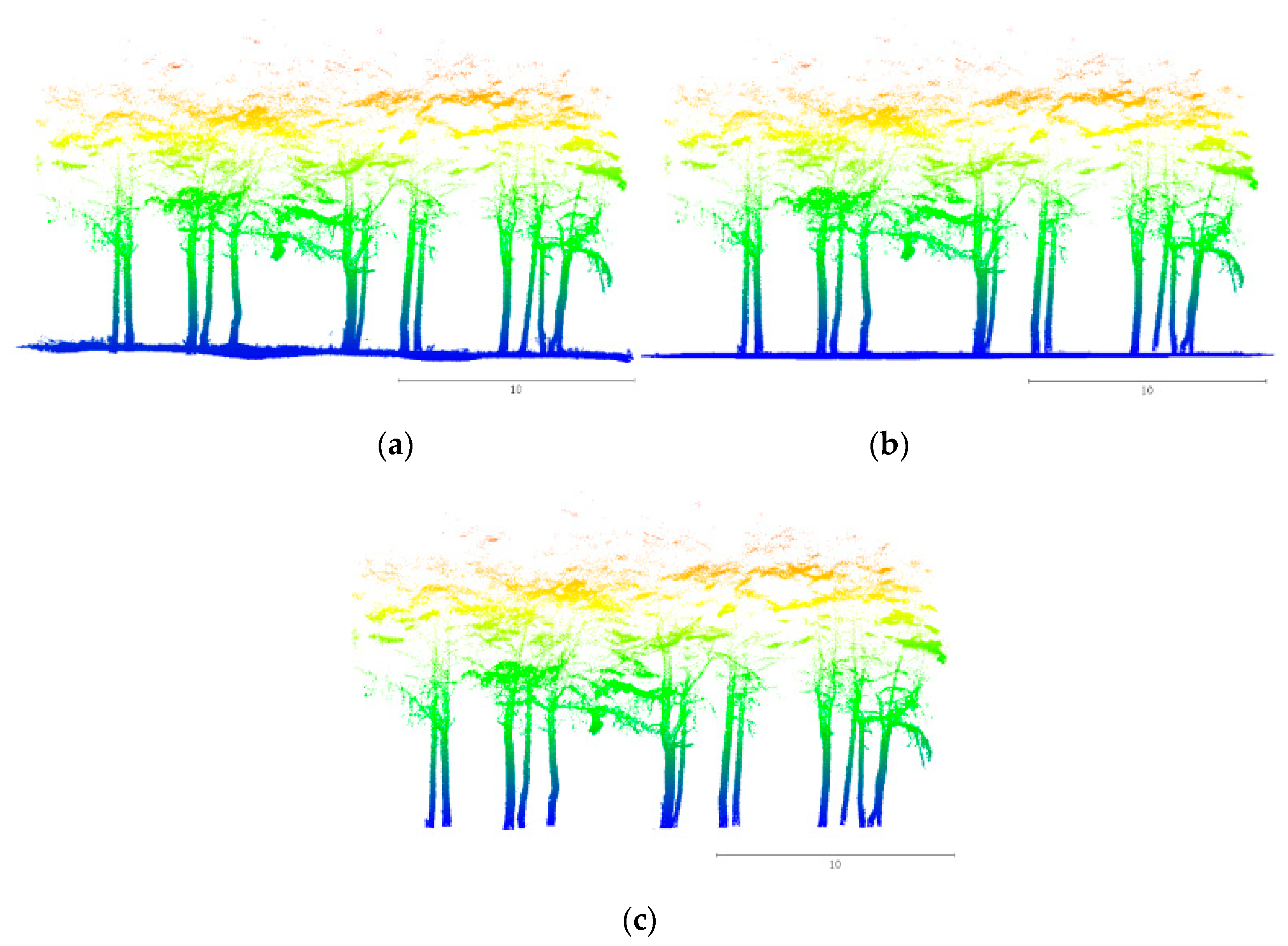
This study mainly focuses on the classification of the stem, branch and leaf point clouds, so the scanned point cloud data needs to be preprocessed by denoising, normalization, and removing the ground point cloud. Firstly, the scanned point cloud data was output from the GeoSLAM desktop software in the format of .las. Then, the CloudCompare software, a 3D point cloud and mesh processing software, was used to denoise the HMLS point cloud and the echo noise that was significantly higher than the crown point cloud layer in the scanned plot was manually deleted. Point cloud normalization was realized by the local minimum method on the platform of Matlab. The specific procedures are as follows: (1) The HMLS point cloud was projected vertically onto the horizontal plane and divided into a 5 cm × 5 cm grid, (2) The minimum z value of all points in the grid was traversed, and the minimum z value was subtracted from all points in the grid in order to get the relative height of the points, and (3) All the grid points were normalized to a unified grid plane to realize point cloud normalization. Finally, the ground points (z < 2 cm) of the normalized tree point clouds were deleted by using the CloudCompare software and the echo point clouds of understory shrubs and weeds were checked and removed. The preprocessed HMLS tree point clouds are shown in Figure 2.
2.3. Model Construction and Evaluation
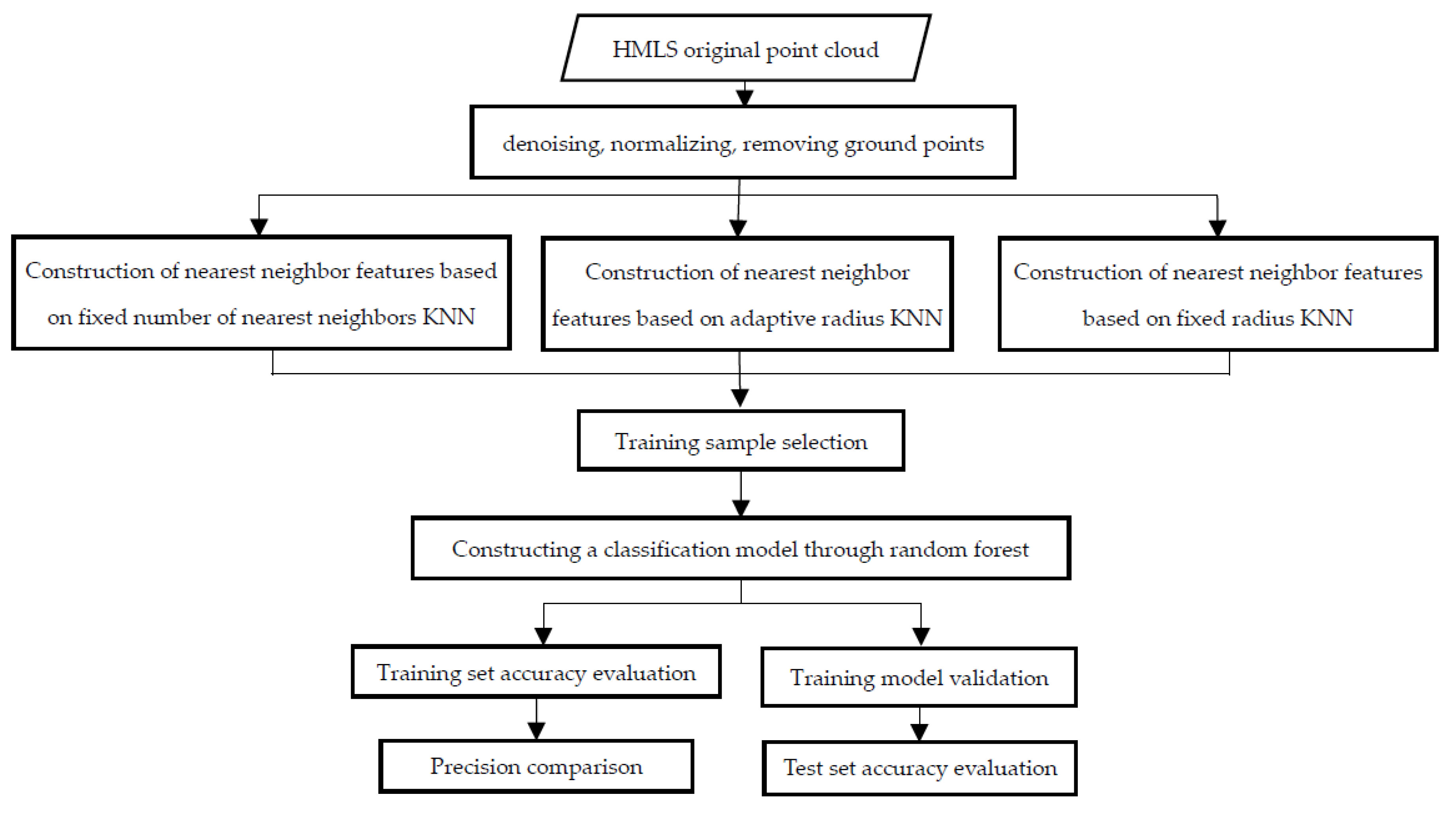
In this study, three types of KNN algorithms (a fixed number of neighbors, an adaptive radius, and a fixed radius) and random forest algorithm were used to classify the stem, branch and leaf point clouds in the forest plot. The KNN algorithms were applied to search for the nearby points within the pre-processed point cloud and the geometric features of the nearest neighbors were calculated for each algorithm. The random forest classifier was then used to train the classification model according to the neighboring geometric features. The HMLS point clouds were divided into stem points and branch & leaf points, and the classification model was extended to the general test sample sets. Finally, the classification accuracy of the model was checked by calculating the accuracy, precision and recall of the classification results, so as to realize the accurate classification of the stem point clouds and the branch & leaf point clouds by HMLS. The technical flow chart is shown in Figure 3.
2.3.1. Neighboring Point Selection
The point cloud neighboring geometric feature is an important indicator that reflects the spatial distribution of the point cloud classification area. It is essential to identify the nearest neighbor points before constructing a point cloud feature vector. The commonly used searching methods of nearest neighbors include three types of KNN algorithms such as based on the fixed number of nearest neighbors, based on a fixed neighborhood radius, and based on an adaptive neighborhood radius. Due to the complex structure of forest plots and the difference of point cloud density among different vertical layers, the above three KNN algorithms were used respectively to search the neighboring points of the point cloud in order to verify their accuracy.
(1) The KNN algorithm based on a fixed number of neighboring points is to set a fixed number (k) of neighboring points to search for neighboring points. In this study, referring to the threshold setting for k in Ma et al. [24] and Wang et al. [25] with TLS data, the search scope of k for HMLS data was defined as [30, 210] with an interval of 30.
(2) The fixed neighborhood radius KNN is to set the neighborhood threshold (r) of each point in the point clouds set to a fixed value, and then find the neighbor points by judging whether the Euclidean distance between the point clouds is less than the fixed threshold. According to the analyses on the geometric features of tree stems, branches and leaves from TLS data by Xia et al. [23] and Zhu et al. [18], a sing-tree stem can present linear feature when r = 6 cm, while branches and leaves can show different near-neighbor geometric features at r = 4 cm and r = 12 cm. In addition, the point cloud density of HMLS data is significantly lower than that of TLS, so more points should be calculated in order to determine the geometric features. Therefore, the scope of the neighborhood threshold r was defined as 5 cm–25 cm with a step length of 5 cm.
(3) The KNN method based on adaptive radius needs to determine the best neighborhood radius of each point by calculating the information entropy of the neighboring point cloud set and then search for the neighboring points. The specific process of adaptive radius KNN algorithm is as follows:
First, the classic principal component analysis (PCA) method is used to calculate the eigenvalues and feature vector of the three-dimensional covariance matrix of neighbor points. The covariance matrix of the nearest neighbor points of the sample point is expressed as
where is the centroid coordinate of the neighboring point of . The covariance matrix is a symmetric positive definite matrix, which can be decomposed as
where R is a matrix composed of feature vectors , representing three orthogonal anisotropy axes of the local spatial distribution of sample points. Λ is a diagonal positive definite matrix composed of eigenvalues (λ1, λ2, λ3), where λ1 > λ2 > λ3, and all are positive values. Let (i = 1, 2, 3), represents the length of three axes. According to the study by Brodu and Lague [26], the following feature indicators were introduced to represent the local spatial characteristics of the sample points:
The basic principles of judging the tree stem or branch and leaf point for any sample point are as follows:
① if , , then is much larger than the other two indicators, the nearest point cloud cluster will be considered to have a linear structure, and is generally classified as tree stem in the tree structure;
② if , , then is much larger than the other two indicators, which indicates that neighboring cluster point cloud has a planar structure, and is generally considered as a ground point cloud or an artificial target point cloud with a planar structure.
③ If , then is much larger than the other two indicators. The neighboring point cloud cluster where the sample point located has divergent local spatial characteristics, and is generally regarded as branch and leaf point clouds.
In order to improve the operating efficiency of the KNN algorithm, a fast KDtree search for point cloud neighbor points based on Euclidean distance was established, and the optimal radius of the nearest neighbor search for each point was determined by calculating the information entropy value of the nearest neighbor point cloud. The information entropy model of the point cloud is established according to Equation (6) [27]. This model can accurately reflect the local spatial characteristics of the point cloud. The smaller the E value, the larger the importance of one dimension than the other two dimensions. Therefore, the neighboring point cloud clusters with specific spatial characteristics can be determined.
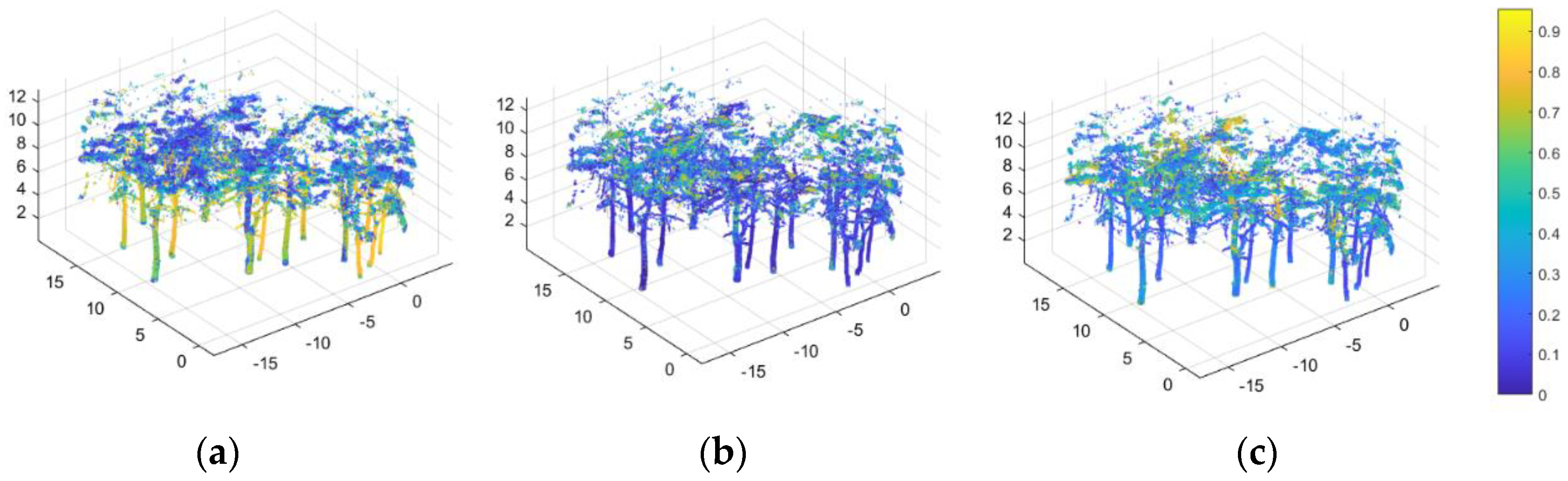
In consideration of the actual situation of the plot, this study calculated the information entropy values of the local neighborhood of the point cloud in the range of 5–25 cm neighborhood radius at an interval of 5 cm, and selected the neighborhood size corresponding to the minimum entropy value as the optimal radius, and finally searched according to the optimal radius to obtain the nearest neighbor point cloud clumps in the adaptive neighborhood. Compared with the traditional nearest neighbor search method, the fast KDtree based on dichotomy has higher efficiency when searching for samples with large data, and can quickly obtain the nearest neighbor point cloud clusters of sample points [28]. After obtaining the optimal radius of the nearest neighbor point cloud cluster of each point, the three spatial features of point clouds , , and were calculated and plotted according to Equations (1)–(5). The results are shown in Figure 4.
2.3.2. Feature Structure
In order to better distinguish the HMLS stem points and branch and leaf points, this study constructed eight geometric features based on previous studies [9,14,20,29], including linear index , planar index , scattered index , curvature , Verticality V, normalized point cloud height , number of neighboring points N, point cloud plane eigenvalue ratio .
The linear index , planar index , and scattered index represent the linear, planar and scattering features of the neighboring point cloud clusters, respectively. Curvature is an important index to measure the bending degree of the neighboring point cloud. The curvature of the stem point is usually less than that of the branch point due to the higher density [30]. The four parameters can be calculated by Equations (7)–(10), where, and represent the three-dimensional eigenvalues of the covariance matrix of the neighboring points.
The verticality V is used to measure the perpendicularity between the normal vector of the neighboring point cloud cluster and the normal vector of the horizontal plane. Since the normal vector of the stem point is parallel to the horizontal plane, its verticality V is usually close to 1, while the verticality of the branch and leaf points is more discrete. The verticality is computed by Equation (11), where is the z-axis component of the normal vector of the neighboring point. The normal vector of the neighboring point is the eigenvector corresponding to the minimum eigenvalue in the covariance matrix of the neighbor point cloud clump, and it is stipulated that the default direction of the normal is the positive direction of the z-axis.
The normalized point cloud height is the height of the point cloud relative to the normalized ground point, which is calculated as Equation (12). The branch and leaf points are generally higher than the stem points. N is the number of neighboring points obtained by fast KDtree search based on a fixed radius neighborhood (Equation (13)). In this study, the radius was set to 15 cm, which means that N is the number of point clouds in a sphere with a radius of 15 cm centered on a specific point. N can also be regarded as the unit density of the point clouds. Generally, the number of neighboring points N of the branch and leaf points is less than that of the stem points for HMLS-based tree point clouds. The ratio is an important parameter to measure the two-dimensional plane characteristics of the point cloud, which is calculated as Equation (14), where are the eigenvalues of the covariance matrix of the horizontal projection of the neighboring point cloud clusters and .
Equations (7)–(14) were applied to calculate the eight feature values of all points in the training sample set and the test sample set and used in the following training and classification analysis.
2.3.3. Selection of Training Sample Set
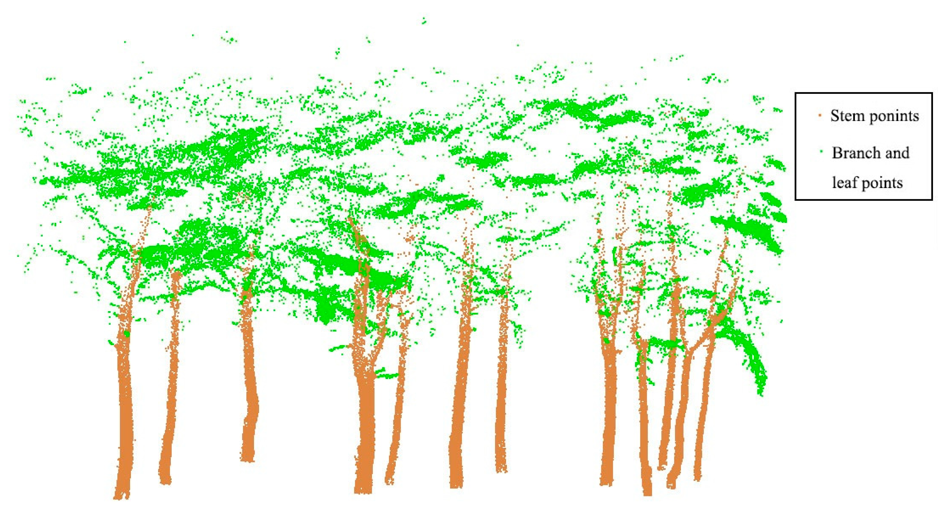
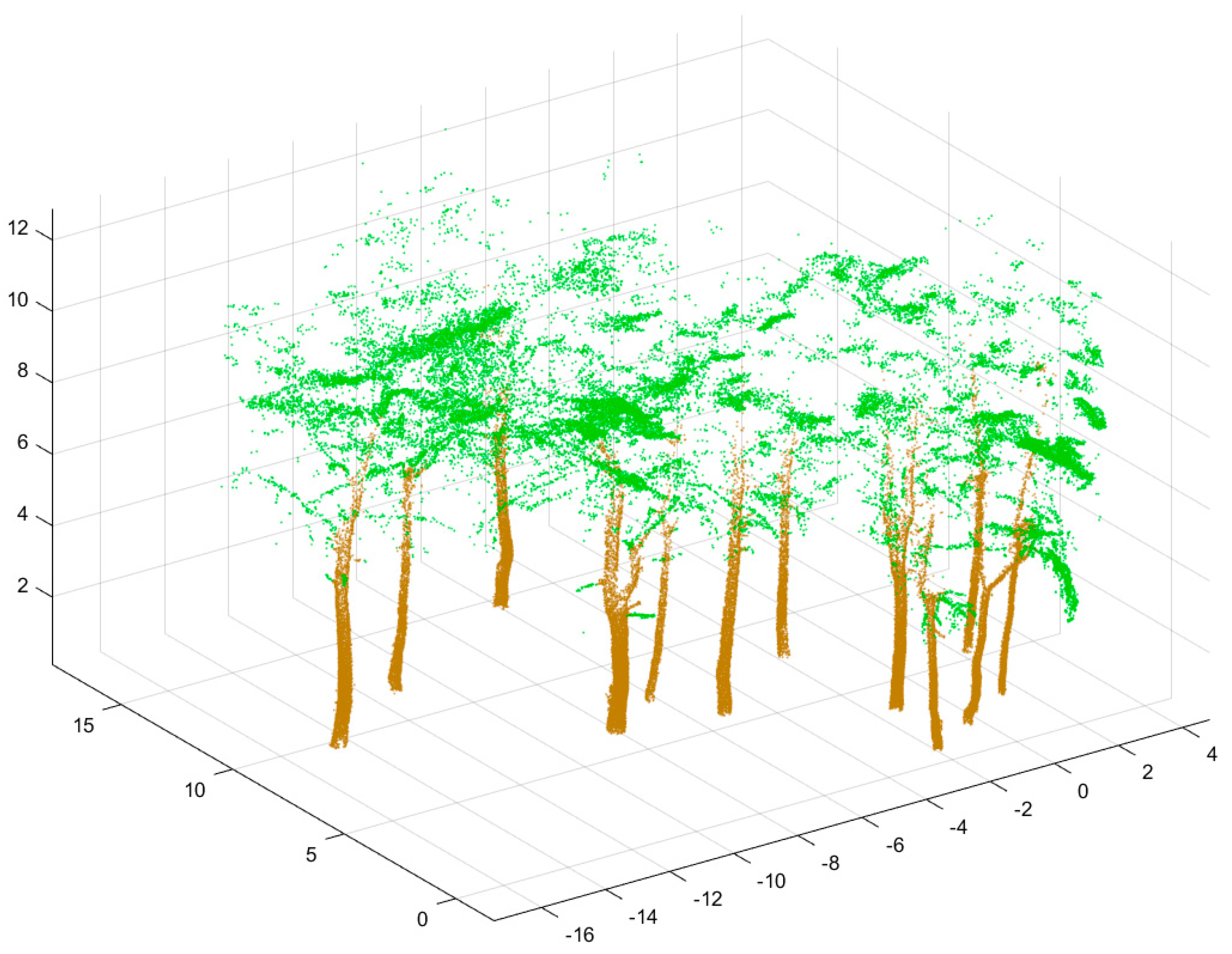
In order to select a reasonable sample set to train the classifier, the marked stem points and branch & leaf points in plot A were selected as the initial training samples. Since there are many clumps in the original point cloud set, it is easy to cause data redundancy if all points were used to train the classifier. Therefore, the original point cloud was randomly sampled at the ratio of 1:3 to obtain the training sample set. A total of 100,000 points were obtained after sampling, including about 70,000 stem points and about 30,000 branch and leaf points. The sample set was then equally divided into ten groups, nine for training and one for verification. The point cloud of the training sample set is shown in Figure 5.
2.3.4. Point Cloud Classification
In this study, the classic random forest algorithm was used to train the classification model. Random Forests is an ensemble classifier, which has been widely applied in forest applications using hyperspectral and LiDAR data [31,32,33]. By integrating multiple weak classifiers (i.e., decision tree), the random forest algorithm is not prone to overfitting when classifying a large data set with high dimensions, so that the overall classification result has high accuracy and good generalization ability [34]. A decision tree can avoid overfitting by pruning, but it will inevitably learn some noise information when training the classification model if there is only one tree. The random forest uses Bagging’s sampling method [35] to combine multiple decision trees, and finally determines the target category by voting (the minority is subordinate to the majority). The specific steps are as follows:
(1) Features importance from random forests was assessed by means of Out-of-Bag Permutation which was used to select relevant features. The oobPermutedPredictorImportance function in Matlab R2019b was used to calculate feature importance. The selected features were used as input data, then Bagging’s sampling method [35] was used for random sampling with replacement, and the decision tree was trained based on the sampling result.
(2) The method of non-replacement sampling was also adopted to randomly select some features (m) from the total features (M) as the reference attributes of node split for the decision tree, where m<<M. The information gain of m features obtained by sampling was calculated, and the feature with the largest information gain value was selected as the node splitting attribute, so as to determine the optimal splitting method of the nodes in the decision tree.
(3) Each node formed by the decision tree was split according to step (2) and grew to the maximum depth. The above steps were repeated to build multiple decision trees and finally generate random forests. When classifying the test data, the classification results given by each decision tree were summarized, and finally the target category of the test data was determined by voting.
The random forest algorithm relies on the randomness of sample selection and feature selection to ensure that the prediction model will not be affected by some specific feature values or some special sample points, reducing the risk of overfitting the prediction model and enhancing the noise-resistance and generalization capabilities. The classification accuracy of random forest mainly depends on the number of integrated weak classifiers [34]. In theory, the larger the number of integrated weak classifiers, the higher the classification accuracy. However, the use of excessive classifiers will increase the computational burden and has very limited improvement in accuracy. After multiple rounds of testing, it was found that a higher accuracy can be reached when the number of classifiers was set to 30, after that the accuracy improvement was very limited. Therefore, the number of random forest integrated decision trees adopted in this study was 30. The Classification Learner APP in Matlab R2019b was used to generate decision trees, and the fitcensemble function was used to realize the integration of weak classifiers (decision trees) and generate random forest classifier.
2.3.5. Accuracy Evaluation
In machine learning, some parameters such as accuracy, precision, and recall are usually calculated to measure the pros and cons of the classification model [36]. In order to test the applicability of the classification model, the above parameters were calculated by constructing a mixed matrix of the classification results of the training samples. The stem points were marked as the positive class, and the branch & leaf points were marked as the negative class. The calculation formulas are shown in Equations (15)–(17), where N represents the total number of samples, TP represents the number of positive samples that are predicted as the positive class, FN represents the number of positive samples that are predicted as the negative class, FP represents the number of negative samples that are predicted as the positive class, and TN represents the number of negative samples that are predicted as the negative class. The accuracy rate (Equation (15)) is an intuitive indicator to measure the classification accuracy of the overall sample, and the accuracy rate (Equation (16)) and recall rate (Equation (17)) are indicators to measure the classification accuracy of a single category. In addition, the classification result of was also calculated (Equation (18)) in this study in order to consider the comprehensive evaluation indicators of precision and recall rate. is the harmonic mean of precision and recall rates, which indicates the credibility of the prediction results. The value ranges of the above indicators are (0, 1). If the value of is closer to 1, then the classification effect will be better.
3. Results Analysis
3.1. Geometric Feature Analysis
The geometric features of HMLS-based tree point cloud were calculated based on three kinds of KNN search methods (a fixed number of neighbor points-based method, Method I; a fixed neighborhood radius-based method, Method II; an adaptive neighborhood radius-based method, Method III). Refering to the previous studies by Wang et al. [25] and Zhu et al. [18] and considering the point cloud density of HMLS data, the parameter settings for the fixed number of near neighbors (k) and fixed radius (r) were 210 and 20 cm, respectively. The importance of feature importance calculated using the Random Forest function is presented in Table 2. ‘Importance’ can be used to predict the explanatory power of the features [18]. It is shown that regardless of the near-neighbor point search algorithm, the most relevant feature was the number of nearby points N, which can also be regarded as the density parameter of the point cloud. Due to the limitation of scanning distance of HMLS, the point cloud density of branches and leaves located in the canopy was far less than that of stems, therefore N was the most important feature. The normalized point cloud height ranked the second in the order of feature importance. This feature can effectively distinguish the stem points below the canopy from the branch and leaf points, but has little difference between the stem points and the branch and leaf points in the canopy. Curvature , perpendicularity V and the ratio of eigenvalues for point cloud plane also play an important role in point cloud classification, indicating that the spatial distribution characteristics of HMLS point clouds of stems, branches and leaves are quite different, which can be used as a basis for classification. Compared with other features, the linear index , planar index and scattered index had relatively lower contribution to the classification accuracy. Since the orders of feature importance were not the same for the three KNN algorithms, all eight features were used as input in the Random Forest classifier.
3.2. Comparison of KNN Search Methods
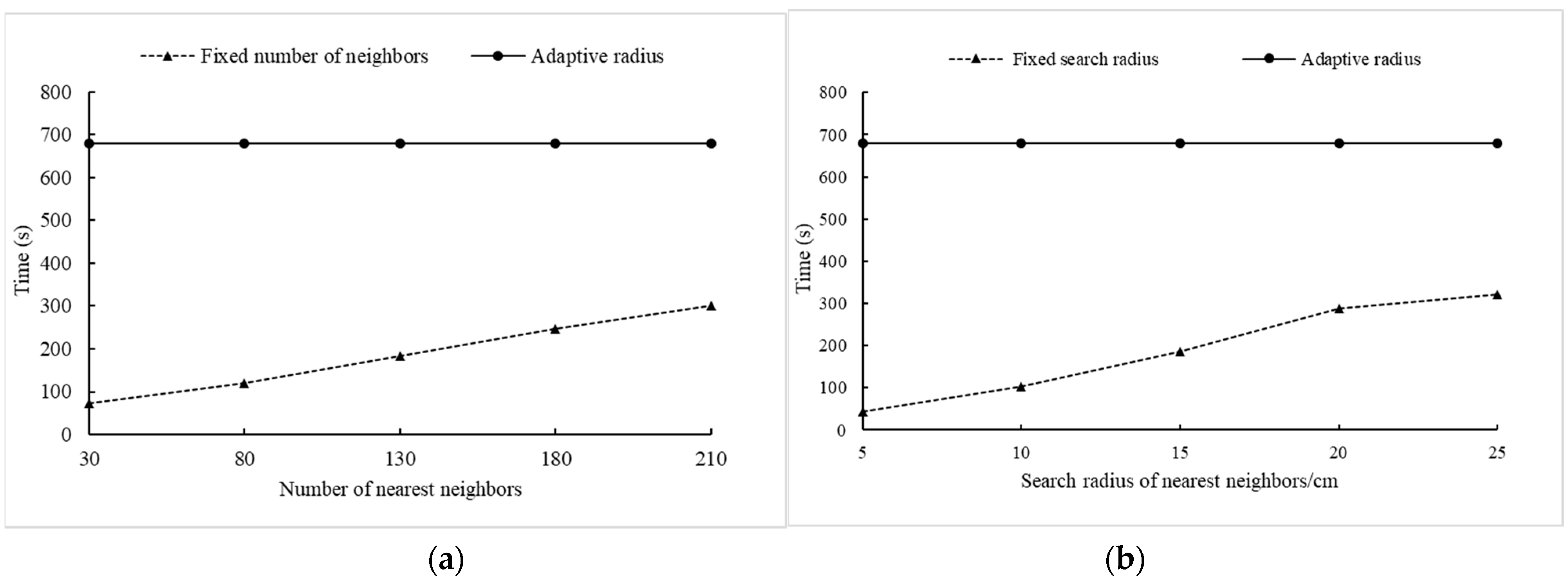
Compared with Method I and Method II, the KNN algorithm with an adaptive neighborhood radius (Method III) is more complicated to search for neighbor points. However, the neighborhood range of each point can be determined more accurately, so that more realistic neighboring geometric features of the tree point clouds can be obtained. The comparison of the three KNN methods in terms of feature calculation time was illustrated in Figure 6. The feature calculation time of Method I and Method II has a positive linear relationship with the number of nearest neighbors and the search radius. With the increase of the search radius and the number of neighboring points, the efficiency of feature calculation gradually decreases. The calculation time of Method III is much longer than the other two methods, and is stable as the search radius and the number of neighboring points increase.
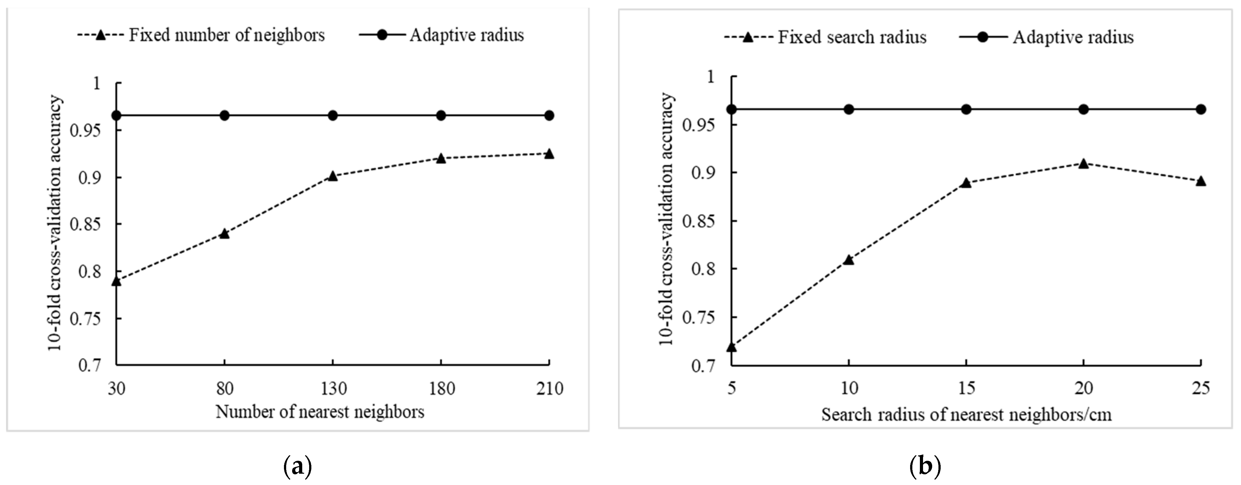
The training sample set was trained respectively based on the eigenvalues calculated by the above three KNN methods and the ten-fold cross-validation accuracy of the classification results were computed [37]. The results are illustrated in Figure 7. It is noted that the classification accuracy using the traditional KNN methods (Method I and Method II) increases with the increase of the search radius and the number of neighbors. The accuracy of the ten-fold cross-validation of the classification results tends to be stable when the neighbor search radius reaches 15 cm or the number of nearest neighbors is 180. The accuracy reaches the highest value when the search radius is set to 20 cm or the number of nearest neighbors is 210. The overall accuracy of Method I is better than that of Method II. However, the optimal accuracy of both traditional KNN search methods is less than that of Method III (0.9659), indicating that the self-adaptive radius KNN search method can better reflect the best neighboring geometric characteristics of the stem points and the branch and leaf points. Therefore, the neighboring geometric feature values calculated by Method III were used in the following analysis.
3.3. Classification Results and Testing Accuracy
According to the calculated neighboring geometric feature values by Method III, the random forest training classifier was used to classify the training samples in the randomly sampled plot A. The results are shown in Figure 8. It can be seen that most of stem point clouds and branch & leaf point clouds in the training sample plot can be effectively classified. However, due to the scanning characteristics of HMLS, that is, as the relative height increases, the point cloud density gradually decreases, and the occlusion effect among crowns, the stem point cloud of crown and the branch & leaf point cloud have a greater similarity in the neighboring point features, so there are some misclassifications. According to the classification results, a mixing matrix was constructed to summarize various accuracy evaluation indicators. The results are shown in Table 3. The accuracy, recall rate and F1Score value of the stem points and branch & leaf points were greater than 0.93, and the overall precision of the classifier reached 0.9659, achieving the purpose of accurate classification on training samples. The accuracy of each index of the stem points was superior to that of the branch & leaf points, the estimated number of stem points was less than the actual number, and the number of branch & leaf points was overestimated, indicating that some stem points were misclassified into branch & leaf points. It can also be found in Figure 8 that in the crown where the density of the point clouds was low, some stem points were partially divided into branch & leaf points.
3.4. Validation Accuracy of the Classification Model
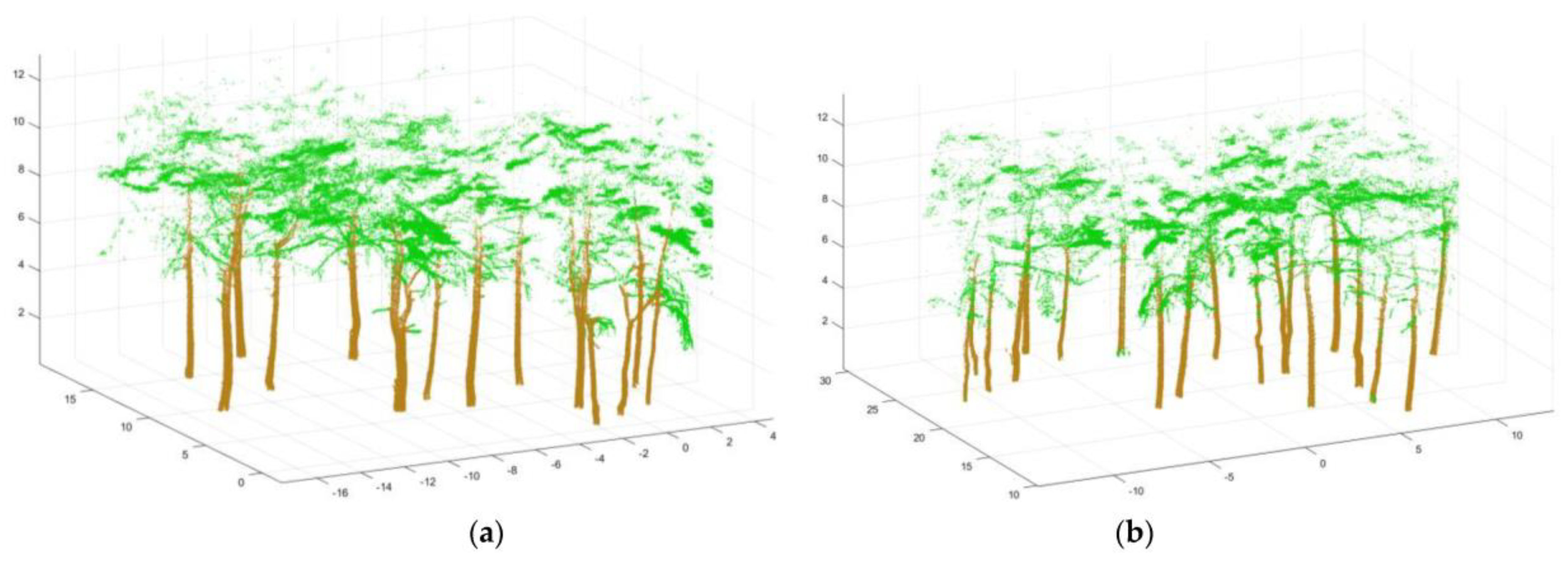
Since HMLS tree point clouds have similar neighbor characteristics, this study used the original point cloud sets of plots A and B as the test sets to verify the accuracy of the adaptive radius KNN search method and the random forest training model. The classification model obtained by the training samples in plot A was applied to plot B in order to test the generalization ability of the model. The classification results of the original HMLS point clouds of plots A and B are shown in Figure 9. The mixing matrix of each test set was constructed and the classification accuracy index was calculated. The results are presented in Table 4 and Table 5. It is noted that the accuracy of the classification of stem points and branch & leaf points in plot A was 0.9730 and 0.9302, respectively, indicating that 97.3% and 93.02% of the classification results estimated by the trainer were correctly classified. The recall rates of the stem points and branch & leaf points were 0.968 3 and 0.940 3, respectively, which showed that the points that were correctly classified account for 96.83% and 94.03% of the actual points in the test set, respectively. In the classification results, the error rates of stem points and branch & leaf points were 2.7% and 6.97%, respectively. Since the training samples came from plot A, the classification model when applied to the test set of plot A showed a better accuracy. The misclassification points mainly occurred in some individual tree crown points (Figure 9a), and most of the remaining points were correctly classified. The overall classification accuracy rate reached 0.9596, which is closer to the accuracy of the training sample (0.9659).
It can be seen from Table 5 that the validation accuracy of the stem points and branch & leaf points in the test set of plot B was 0.9326 and 0.9006, respectively; the recall of stem, branch and leaf points was 0.9362 and 0.8952, respectively; and the misclassification rates of the two types of points were 6.74% and 9.94%, respectively. As shown in Figure 9b, the stem located in the crown was usually surrounded by dense branches and leaves, and the point clouds density of the stem will also decrease with the increase of the relative height, which adds uncertainty to the calculation of the neighboring geometric feature values of the crown stem points, resulting in more misclassification of stem points in the crown. Even though the overall accuracy rate of the test set of plot B (0.9201) was relatively lower than that of the training set (0.9659) and test set of plot A (0.9596), it can still be accepted.
4. Discussion
The realization of rapid segmentation of tree point cloud is of great significance for the application of HMLS in forestry practice. The selection of appropriate algorithm for calculating the geometric features of neighborhood points is the key to the correct classification of stem, branch and leaf points for HMLS-based tree point cloud. In this study, the calculation time and classification accuracy of different classification models based on different KNN algorithms and random forest classifier was compared. Although the training time of the fixed number of near-neighbors-based KNN method (Method I) and fixed radius-based KNN method (Method II) was much shorter, especially with fewer number of neighbor points or smaller neighborhood radius (Figure 6), their classification accuracy were inferior to the adaptive radius-based KNN method (Method III), even at the optimal number of neighbor points (k = 210) or neighborhood radius (r = 20 cm) (Figure 7). Moreover, when searching for the neighborhood of a point cloud training set with unknown feature information, multiple attempts were needed to set the parameters for Methods I and II in order to obtain the optimal search radius or the optimal number of neighbors. Therefore, the adaptive radius-based KNN method was the best classification model for HMLS-based tree point cloud. Zhu et al. [18] also reported a similar result that the adaptive radius near-neighbor search method outperformed the fixed radius near-neighbor search method in discriminating foliage and woody materials.
It is useful to compare the classification accuracy in this study with those previous studies from TLS point cloud, since the classification of tree point cloud from HMLS data is rarely documented. Zheng et al. [38] used a pointwise classification method to recognize foliar, woody and ground points from TLS data, resulting in an overall accuracy of 85.5% for a broadleaf forest plot with high density (LAIe = 4.15). Zhu et al. [18] used an adaptive radius near-neighbor search algorithm to obtain both geometric and radiometric features for discriminating between foliar, woody and ground materials from TLS data. An average overall accuracy of 84.4% was achieved across all experimental plots with various vegetation types (conifer, broadleaf, mixed forest), which was close to the accuracy of Zheng et al. [38]. Ma et al. [39] applied a geometric-based automatic forest point classification algorithm to separate the photosynthetic (leaf and grass points) and non-photosynthetic (stem and branch points) components from TLS data. The overall accuracy of the three plots were 84.3% (high-density forest plot, LAI = 4.15), 94.4% (medium-density forest plot, LAI = 3.65), and 97.8% (low-density forest plot, LAI = 3.13), respectively. They also found that tree species almost had little effects on the classification accuracy, as shown by the overall accuracy for coniferous (93.09%) and broadleaf (94.96%) trees. Our study results showed that the classification accuracy of HMLS-based tree point clouds from two test sample plots was 0.9596 and 0.9201, respectively, by using the best classification model. The difference in accuracy can be attributed to several factors such as data preprocessing, forest structure and forest conditions, scanning approach, etc. In the previous studies [18,38,39], TLS-based point clouds were usually classified into three categories, i.e., foliar, woody and ground points. In our study, the HMLS tree point cloud was preprocessed by removing the ground points and the rest were classified into two categories, including stem points and branch and leaf points, therefore less noise was introduced and the classification accuracy was improved. Our study plots were homogeneous Pinus tabulaeformis plantation with low density (LAI = 2.63), and the serpentine scanning approach was adopted to reduce the impact of tree occlusion, resulting in a relative high-quality HMLS data.
It is also noted that there were still many misclassifications due to the occlusion effect and the detection accuracy of the point cloud in the upper part of the tree stem was relatively lower. The accuracy of the best classification model in this study decreased slightly when applied to the test sets. Similar conclusions can also be found in other tree point cloud classification studies. For example, Ma et al. [24] constructed multiple neighboring geometric features and used random forest algorithm for feature selection and classification. The accuracy of the classification results for the training set was as high as 93%, but dropped to 60% when applied in the other forest plots with different forest structures. In addition, the size of the training sample set in this study was relatively smaller. Theoretically, the more training samples, the closer to the real situation. However, excessive training samples will cause too much calculation during training, resulting in data redundancy, while insufficient number of samples will affect the universality of the samples, which is unfavorable to the generalization of the classification model. Therefore, an appropriate sample size should be determined to get the best training results.
Future research can be conducted to test the difference of different sample sizes on the classification accuracy of the best classification model. In addition, the classification accuracy should be validated for different forest structures and stand conditions in order to expand the application of HMLS-based tree point cloud classification model in the context of complex forest environment.
5. Conclusions
This paper has compared the classification accuracy of different classification models which consist of different KNN search methods and random forest classifier. The main conclusions from this study are as follows:
(1) Compared with the traditional nearest neighbor search methods based on a fixed number of neighbor points (Method I) and a fixed neighborhood radius (Method II), the nearest neighbor search method based on the adaptive neighborhood radius (Method III) can better reflect the true neighboring characteristics of the point cloud. Therefore, Method III, the nearest neighbor search method based on the adaptive neighborhood is a more suitable choice for searching for the nearby points in HMLS tree point cloud.
(2) According to the feature importance values derived from Random Forest classifier, the most relevant feature was the number of nearby points, followed by the normalized point cloud height, regardless of the KNN algorithms. The orders of the rest geometric features were slightly different among the KNN algorithms. It is shown that the ratio of eigenvalues for point cloud plane, perpendicularity and curvature also played an important role in point cloud classification. Compare to the other features, the linear index, planar index and scattered index contributed less to the classification accuracy.
(3) The best classification model based on the adaptive radius KNN algorithm (Method III) and random forest algorithm can effectively achieve classification of HMLS-based tree point clouds. The validation accuracy of the best classification model on the test sample plots was satisfactory, indicating that the classification model was stable and can be applied to other HMLS-based tree point clouds with similar forest structure and stand conditions.
Author Contributions
Conceptualization, W.L.; Formal analysis, W.F. and J.W.; Funding acquisition, W.L.; Investigation, W.F., H.L. and Y.X.; Methodology, W.L., W.F. and J.W.; Project administration, W.L.; Supervision, J.W.; Validation, W.F., H.L. and Y.X.; Writing—original draft, W.L. and W.F.; Writing—review & editing, J.W. All authors have read and agreed to the published version of the manuscript.
Funding
This research was funded by the National Natural Science Foundation of China, Grant Number: 31971574; the Joint Project of the Natural Science Foundation of Heilongjiang Province, Grant Number: LH2020C049; and the Fundamental Research Funds for Central Universities, Grant Number: 2572019BL03.
Data Availability Statement
The data presented in this study are available on request from the corresponding author. The data are not publicly available due to privacy or ethical restrictions.
Acknowledgments
The authors thank Beijing MAG Tianhong Science & Technology Development Co., Ltd. for support in data collection.
Conflicts of Interest
The authors declare no conflict of interest.
References
- Ryding, J.; Williams, E.; Smith, M.J.; Eichhorn, M.P. Assessing handheld mobile laser scanners for forest surveys. Remote Sens. 2015, 7, 1095–1111. [Google Scholar] [CrossRef] [Green Version]
- Hyyppä, E.; Yu, X.; Kaartinen, H.; Hakala, T.; Kukko, A.; Vastaranta, M.; Hyyppä, J. Comparison of backpack, handheld, under-canopy UAV, and above-canopy UAV laser scanning for field reference data collection in boreal forests. Remote Sens. 2020, 12, 3327. [Google Scholar] [CrossRef]
- Hyyppä, E.; Kukko, A.; Kaijaluoto, R.; White, J.C.; Wulder, M.A.; Pyörälä, J.; Liang, X.; Yu, X.; Wang, Y.; Kaartinen, H.; et al. Accurate derivation of stem curve and volume using backpack mobile laser scanning. ISPRS J. Photogramm. Remote Sens. 2020, 161, 246–262. [Google Scholar] [CrossRef]
- Balenović, I.; Liang, X.; Jurjević, L.; Hyyppä, J.; Seletković, A.; Kukko, A. Hand-held personal laser scanning-current status and perspectives for forest inventory application. Croat. J. For. Eng. 2021, 42, 165–183. [Google Scholar] [CrossRef]
- Balado, J.; Díaz-Vilariño, L.; Arias, P.; González-Jorge, H. Automatic classification of urban ground elements from mobile laser scanning data. Autom. Constr. 2018, 86, 226–239. [Google Scholar] [CrossRef] [Green Version]
- Naesset, E.; Bollandsas, O.M.; Gobakken, T.; Gregoire, T.G.; Stahl, G. Model-assisted estimation of change in forest biomass over an 11 year period in a sample survey supported by airborne LiDAR: A case study with post-stratification to provide “activity data”. Remote Sens. Environ. 2013, 128, 299–314. [Google Scholar] [CrossRef] [Green Version]
- Cabo, C.; Del Pozo, S.; Rodríguez-Gonzálvez, P.; Ordóñez, C.; González-Aguilera, D. Comparing terrestrial laser scanning (TLS) and wearable laser scanning (WLS) for individual tree modeling at plot level. Remote Sens. 2018, 10, 540. [Google Scholar] [CrossRef] [Green Version]
- Giannetti, F.; Puletti, N.; Quatrini, V.; Travaglini, D.; Bottalico, F.; Corona, P.; Chirici, G. Integrating terrestrial and airborne laser scanning for the assessment of single-tree attributes in Mediterranean forest stands. Eur. J. Remote Sens. 2018, 51, 795–807. [Google Scholar] [CrossRef] [Green Version]
- Bauwens, S.; Bartholomeus, H.; Calders, K.; Lejeune, P. Forest inventory with terrestrial LiDAR: A comparison of static and hand-held mobile laser scanning. Forests 2016, 7, 127. [Google Scholar] [CrossRef] [Green Version]
- Chen, S.; Liu, H.; Feng, Z.; Shen, C.; Chen, P. Applicability of personal laser scanning in forestry inventory. PLoS ONE 2019, 14, e0211392. [Google Scholar]
- Gollob, C.; Ritter, T.; Nothdurft, A. Forest inventory with long range and high-speed personal laser scanning (PLS) and simultaneous localization and mapping (SLAM) technology. Remote Sens. 2020, 12, 1509. [Google Scholar] [CrossRef]
- Oveland, I.; Hauglin, M.; Giannetti, F.; Schipper Kjørsvik, N.; Gobakken, T. Comparing three different ground based laser scanning methods for tree stem detection. Remote Sens. 2018, 10, 538. [Google Scholar] [CrossRef] [Green Version]
- Wang, C.; Wen, C.; Dai, Y.; Yu, S.; Liu, M. Urban 3D modeling using mobile laser scanning: A review. Virtual Real. Intell. Hardw. 2020, 2, 175–212. [Google Scholar] [CrossRef]
- Zhang, W.; Wan, P.; Wang, T.; Cai, S.; Chen, Y.; Jin, X.; Yan, G. A novel approach for the detection of standing tree stems from plot-level terrestrial laser scanning data. Remote Sens. 2019, 11, 211. [Google Scholar] [CrossRef] [Green Version]
- Lalonde, J.F.; Vandapel, N.; Huber, D.F.; Hebert, M. Natural terrain classification using three-dimensional ladar data for ground robot mobility. J. Field Robot. 2006, 23, 839–861. [Google Scholar] [CrossRef]
- Liang, X.; Kankare, V.; Yu, X.; Hyyppä, J.; Holopainen, M. Automated stem curve measurement using terrestrial laser scanning. IEEE Trans. Geosci. Remote Sens. 2014, 52, 1739–1748. [Google Scholar] [CrossRef]
- Kelbe, D.; van Aardt, J.; Romanczyk, P.; van Leeuwen, M.; Cawse-Nicholson, K. Single-scan stem reconstruction using low-resolution terrestrial laser scanner data. IEEE J. Sel. Top. Appl. Earth Obs. Remote Sens. 2015, 8, 3414–3427. [Google Scholar] [CrossRef]
- Zhu, X.; Skidmore, A.K.; Darvishzadeh, R.; Niemann, K.O.; Liu, J.; Shi, Y.; Wang, T. Foliar and woody materials discriminated using terrestrial LiDAR in a mixed natural forest. Int. J. Appl. Earth Obs. Geoinf. 2018, 64, 43–50. [Google Scholar] [CrossRef]
- Arachchige, N.H. Automatic Tree Dectection-A Geometric Feature Based Approach for MLS Point Clouds; ISPRS Annals of the Photogrammetry, Remote Sensing and Spatial Information Sciences: Antalya, Turkey, 2013; Volume II-5/W2, pp. 109–114. [Google Scholar]
- Zhang, A.; Li, W.; Duan, Y.; Meng, X.; Wang, S.; Li, H. Point cloud classification based on point feature histogram. J. Comput. Aided Des. Comput. Graph. 2016, 28, 795–801. [Google Scholar]
- Xu, S.; Xu, S.; Ye, N.; Zhu, F. Automatic extraction of street trees’ nonphotosynthetic components from MLS data. Int. J. Appl. Earth Obs. Geoinf. 2018, 69, 64–77. [Google Scholar] [CrossRef]
- Ye, W.; Qian, C.; Tang, J.; Liu, H.; Fan, X.; Liang, X.; Zhang, H. Improved 3D stem mapping method and elliptic hypothesis-based DBH estimation from terrestrial laser scanning Data. Remote Sens. 2020, 12, 352. [Google Scholar] [CrossRef] [Green Version]
- Xia, S.; Wang, C.; Pan, F.; Xi, X.; Zeng, H.; Liu, H. Detecting stems in dense and homogeneous forest using single-scan TLS. Forests 2015, 6, 3923–3945. [Google Scholar] [CrossRef] [Green Version]
- Ma, Z.; Pang, Y.; Li, Z.; Lu, H.; Liu, L.; Chen, B. Fine classification of near-ground point cloud based on terrestrial laser scanning and detection of forest fallen wood. J. Remote Sens. 2019, 23, 743–755. [Google Scholar]
- Wang, X.; Xing, Y.; You, H.; Xing, T.; Shu, S. TLS point cloud classification of forest based on nearby geometric features. J. Beijing For. Univ. 2019, 41, 138–146. [Google Scholar]
- Brodu, N.; Lague, D. 3D terrestrial lidar data classification of complex natural scenes using a multi-scale dimensionality criterion: Applications in geomorphology. Isprs J. Photogramm. Remote Sens. 2012, 68, 121–134. [Google Scholar] [CrossRef] [Green Version]
- Demantké, J.; Mallet, C.; David, N.; Vallet, B. Dimensionality Based Scale Selection in 3D Lidar Point Clouds. Proc. ISPRS Workshop Laser Scanning 2011, 38, 97–102. [Google Scholar] [CrossRef] [Green Version]
- Muja, M.; Lowe, D.G. Fast Approximate Nearest Neighbors with Automatic Algorithm Configuration. In Proceedings of the Fourth International Conference on Computer Vision Theory & Applications, Lisbon, Portugal, 5–8 February 2009; Volume 2, pp. 331–340. [Google Scholar]
- Xiao, Y.; Hu, S.; Xiao, S.; Zhang, A. A fast statistical method of tree information from 3D laser point clouds. Chin. J. Lasers 2018, 45, 266–272. [Google Scholar]
- Olofsson, K.; Holmgren, J. Single tree stem profile detection using terrestrial laser scanner data, flatness saliency features and curvature properties. Forests 2016, 7, 207. [Google Scholar] [CrossRef]
- Belgiu, M.; Drăguţ, L. Random forest in remote sensing: A review of applications and future directions. ISPRS J. Photogramm. Remote Sens. 2016, 114, 24–31. [Google Scholar] [CrossRef]
- Bigdeli, B.; Samadzadegan, F.; Reinartz, P. Fusion of hyperspectral and LIDAR data using decision template-based fuzzy multiple classifier system. Int. J. Appl. Earth Obs. Geoinf. 2015, 38, 309–320. [Google Scholar] [CrossRef]
- Koenig, K.; Höfle, B.; Hämmerle, M.; Jarmer, T.; Siegmann, B.; Lilienthal, H. Comparative classification analysis of post-harvest growth detection from terrestrial LiDAR point clouds in precision agriculture. ISPRS J. Photogramm. Remote Sens. 2015, 104, 112–125. [Google Scholar] [CrossRef]
- Breiman, L. Random forests. Mach. Learn. 2001, 45, 5–32. [Google Scholar] [CrossRef] [Green Version]
- Breiman, L. Bagging predictors. Mach. Learn. 1996, 24, 123–140. [Google Scholar] [CrossRef] [Green Version]
- Zhou, Z. Machine Learning; Tsinghua University Press: Beijing, China, 2016; pp. 29–33. [Google Scholar]
- Demsar, J. Statistical comparisons of classifiers over multiple data sets. J. Mach. Learn. Res. 2006, 7, 1–30. [Google Scholar]
- Zheng, G.; Ma, L.; He, W.; Eitel, J.U.; Moskal, L.M.; Zhang, Z. Assessing the contribution of woody materials to forest angular gap fraction and effective leaf area index using terrestrial laser scanning data. IEEE Trans. Geosci. Remote Sens. 2016, 54, 1475–1487. [Google Scholar] [CrossRef]
- Ma, L.; Zheng, G.; Eitel, J.U.H.; Moskal, L.M.; He, W.; Huang, H. Improved salient feature-based approach for automatically separating photosynthetic and nonphotosynthetic components within terrestrial lidar point cloud data of forest canopies. IEEE Trans. Geosci. Remote Sens. 2016, 54, 679–696. [Google Scholar] [CrossRef]
Figure 1.
Location of the study area.

Figure 2.
HMLS point cloud preprocessing. (a) Original point cloud; (b) Normalized point cloud; (c) Point cloud after removing ground points.
Figure 2.
HMLS point cloud preprocessing. (a) Original point cloud; (b) Normalized point cloud; (c) Point cloud after removing ground points.

Figure 3.
Technical flow chart.

Figure 4.
Schematic diagram of point clouds characteristic index. (a) (b) (c) .

Figure 5.
Sample points in the training set.

Figure 6.
Comparison of feature calculation time between adaptive radius search and traditional KNN search methods. (a) Fixed number of neighbors (Method I) vs. adaptive radius search (Method III), (b) Fixed search radius (Method II) vs. adaptive radius search (Method III).
Figure 6.
Comparison of feature calculation time between adaptive radius search and traditional KNN search methods. (a) Fixed number of neighbors (Method I) vs. adaptive radius search (Method III), (b) Fixed search radius (Method II) vs. adaptive radius search (Method III).

Figure 7.
Comparison of training accuracy between adaptive radius search and traditional KNN search methods. (a) Fixed number of neighbors (Method I) and adaptive radius search (Method III), (b) Fixed search radius (Method II) and adaptive radius search (Method III).
Figure 7.
Comparison of training accuracy between adaptive radius search and traditional KNN search methods. (a) Fixed number of neighbors (Method I) and adaptive radius search (Method III), (b) Fixed search radius (Method II) and adaptive radius search (Method III).

Figure 8.
Classification results of the training sample set.

Figure 9.
Classification results of the test sets. (a) Test set A. (b) Test set B.


Table 1.
Technical specifications of ZEB-REVO handheld laser scanning system.
| Performance Index | ZEB-REVO |
|---|---|
| Maximum Range (m) | 30 (15–20 outdoor) |
| Range accuracy (cm) | 1–3 |
| Acquisition rate (points/second) | 43,200 |
| Scanner line speed (Hz) | 100 |
| Field of view (°) | 270/360 |
| Scanning resolution (°) | 0.625/1.8 |
| Laser wavelength (nm) | 905 |
| Laser safety classification | Class I Eye Safe |
| Beam divergence (mrad) | 1.7 × 14 |
Table 2.
Feature importance values derived from Random Forest classifier.
| Methods | V | N | ||||||
|---|---|---|---|---|---|---|---|---|
| Method I (k = 210) | 5.7548 | 1.5357 | 1.2580 | 2.1846 | 1.8693 | 4.3016 | 3.8248 | 7.2565 |
| Method II (r = 20 cm) | 3.9500 | 2.6005 | 1.7661 | 2.2384 | 3.6150 | 2.5957 | 2.8702 | 5.3481 |
| Method III | 6.1417 | 1.1964 | 1.8286 | 1.6456 | 2.1942 | 2.9819 | 4.6479 | 9.5896 |
Table 3.
Classification accuracy index of the training samples.
| Category | Estimated Quantity | Correctly Estimated Quantity | Actual Quantity | Precision | Recall | F1Score | Accuracy |
|---|---|---|---|---|---|---|---|
| Stem points | 67,571 | 66,240 | 68,304 | 0.9803 | 0.9698 | 0.9750 | 0.9659 |
| Branch & leaf points | 32,413 | 30,349 | 31,680 | 0.9363 | 0.9580 | 0.9470 |
Table 4.
Mixing matrix and precision value of test set A.
| Actual Class | Stem Points | Branch and Leaf Points | Total | Precision | |
|---|---|---|---|---|---|
| Estimated Class | |||||
| Stem points | 200,340 | 5554 | 205,894 | 0.9730 | |
| B&F points | 6560 | 87,506 | 94,066 | 0.9302 | |
| Total | 206,900 | 93,060 | 299,960 | ||
| Recall | 0.9683 | 0.9403 | 0.9596 | ||
Table 5.
Mixing matrix and precision value of test set B.
| Actual Class | Stem Points | Branch and Leaf Points | Total | Precision | |
|---|---|---|---|---|---|
| Estimated Class | |||||
| Stem points | 117,787 | 8512 | 126,300 | 0.9326 | |
| B&F points | 8023 | 72,696 | 80,719 | 0.9006 | |
| Total | 125,811 | 81,208 | 207,019 | ||
| Recall | 0.9362 | 0.8952 | 0.9201 | ||
Publisher’s Note: MDPI stays neutral with regard to jurisdictional claims in published maps and institutional affiliations. |
© 2021 by the authors. Licensee MDPI, Basel, Switzerland. This article is an open access article distributed under the terms and conditions of the Creative Commons Attribution (CC BY) license (http://creativecommons.org/licenses/by/4.0/).
Share and Cite
MDPI and ACS Style
Lin, W.; Fan, W.; Liu, H.; Xu, Y.; Wu, J. Classification of Handheld Laser Scanning Tree Point Cloud Based on Different KNN Algorithms and Random Forest Algorithm. Forests 2021, 12, 292. https://0-doi-org.brum.beds.ac.uk/10.3390/f12030292
AMA Style
Lin W, Fan W, Liu H, Xu Y, Wu J. Classification of Handheld Laser Scanning Tree Point Cloud Based on Different KNN Algorithms and Random Forest Algorithm. Forests. 2021; 12(3):292. https://0-doi-org.brum.beds.ac.uk/10.3390/f12030292
Chicago/Turabian StyleLin, Wenshu, Weiwei Fan, Haoran Liu, Yongsheng Xu, and Jinzhuo Wu. 2021. "Classification of Handheld Laser Scanning Tree Point Cloud Based on Different KNN Algorithms and Random Forest Algorithm" Forests 12, no. 3: 292. https://0-doi-org.brum.beds.ac.uk/10.3390/f12030292
Note that from the first issue of 2016, this journal uses article numbers instead of page numbers. See further details here.