Benchmarking Procurement Cost Saving Strategies for Wood Supply Chains

Abstract

Intense international competition pushes the actors of wood supply chains to implement efficient wood supply chain management incorporating coordinated cost-saving strategies to remain competitive. In order to observe the effects of individual and coordinated decision making, mixed-integer programming models for forestry, round-wood transport, and the wood-based industry were developed and integrated. The models deal with operational planning issues regarding production, harvest, and transport and are solved sequentially for individual cost optimization of each wood supply chain actor as well as simultaneously by a combined model representing joint cost optimization in an integrated wood supply chain. This allows for the first time, benchmarking relative cost-saving potential of the wood procurement strategies coordinated transports, integrated supply chains, satellite stockyards, and higher truck payloads within a single case study setting. Based on case study data from southern Austria, results show the advantages of an integrated supply chain with a cost-saving potential of up to 24%. Higher truck payloads reinforce this potential and enable up to 40% savings compared to the predominant wood procurement situation in Central Europe. Wood supply chain integration for Central European circumstances seems to be feasible only for a limited consortium of a few companies, for example when restricted to a wood-buying syndicate supplying several industry plants or a few large forest enterprises, especially as both groups are commonly steering wood transport on their own. Consequently, further research on the challenging task of implementing integrated supply chains using the opportunities of digitalization to realize existing cost savings potential by deepening cooperation and intensifying information exchange is needed.

1. Introduction

Wood supply chains are dynamic networks of complex information and material flows between forestry, transport, and industry stakeholders. Contrary to supply chains of other industries (e.g., car, electronics), uncoordinated decision making focusing on individual interests of single actors in planning, designing, operating, controlling, and monitoring the wood supply chain dominates wood supply chains in Central Europe. Wood supply chain actors pushing their own agendas and optimizing solely their own performance impose constraints on other actors and lead to inefficiencies harming the performance and competitiveness of the entire supply chain. Examples of integrated wood supply chains, particularly in Northern Europe, Canada, and Chile, indicate a competitive advantage through cooperation and coordinated decisions making. Consequently, benchmarking promising procurement cost-saving strategies enables wood supply chain stakeholders to implement efficient and coordinated wood supply chain management to remain competitive in an intensifying international competition environment.

In the scientific literature on wood supply chain management, operation research methods were used to observe operational, tactical, and strategic planning problems and applications [1,2,3]. Related literature reviews concentrated on optimizing wood transport [4], forest biomass supply chains [5], transport logistics in Nordic countries [6] as well as unimodal and multimodal wood transport including terminal logistics [7]. Research articles focused on analyzing procurement cost-saving strategies such as transport coordination, supply chain integration, integrating satellite stockyards, or higher truck payloads with operations research methods.

The formulation of requirements for timber transport vehicle routing [8] encouraged researchers to focus on transport coordination strategies reducing transport costs. Column generation-based solution approaches were used to solve the log truck scheduling problem [9] as well as integrating backhaul transport planning in forestry [10] and showed cost savings in Swedish case studies. Cost savings in Austrian case studies were achieved by a three-stage planning approach consisting of a transport problem, timber transport order smoothing problem, and timber transport vehicle routing problem [11] with a Tabu search-based solution procedure [12]. Combining optimization [13] with Discrete Event Simulation enabled including stochastic effects in short-term transport planning to reduce truck queuing and waiting times at industries in a Portuguese case study setting [14].

Wood supply chain integration considering strategic and tactical planning was mainly observed with mixed-integer programming models applying case study data from Australia [15], Sweden [16,17], Canada [18], and Chile [19,20]. Moreover, linear programming approaches were utilized to model tactical planning decisions in the Chilean sawmill industry [21] and strategic decisions for integrated harvest and production planning in Canada [22]. Strategic decisions for a vertically integrated paper mill were considered with an analytical model combining forest economics and operations management perspectives [23].

The potential of satellite stockyards was observed by solving the terminal location problem in the forest fuel supply network based on a mixed-integer linear programming model [24]. Others used a multi-period model to decide on the location of stockyards to integrate seasonal payload restrictions and enable transport cost savings by natural wood drying [25].

Truck and train terminals as well as the effects of higher truck payloads (i.e., up to 50 t) on critical key performance indicators were analyzed in Discrete Event Simulation models for Austrian case study settings of multi-echelon [26] and multimodal [27] wood supply chains. These built on an earlier model [28] enabling game-based stakeholder workshops [29]. For Finish case study settings, high-capacity truck transportation systems of up to 84 t were observed in Discrete Event Simulation [30] and Agent-based Simulation models [31]. A linear programming model was used for an Australian case study setting comparing five truck configurations with gross vehicle weights between 42.5 and 79 t [32].

The literature review on procurement cost-saving strategies showed the suitability of the mixed-integer programming method but also revealed that case studies concentrated to a large extend only on a single cost-saving strategy. Therefore, the variety of research methods, models, and case study settings constrains a direct comparison of the impacts of different procurement cost-saving strategies, which displays a considerable research gap. Consequently, the goal of this study is to benchmark procurement cost-saving strategies in an identical case study setting. This enables answering the research question: What is the relative cost-saving potential of coordinated transport, higher truck payloads, integrated supply chains, integrated supply chains combined with higher truck payloads, and satellite stockyards?

Therefore, a mixed-integer programming approach was applied to implement operational production, harvest, and transport planning models and solve them sequentially for individual cost optimization of each wood supply chain actor as well as simultaneously by a combined model representing joint cost optimization in an integrated wood supply chain. This enabled direct comparisons of uncoordinated decision making of forestry, transport, and industry with coordinated decision making in an integrated supply chain to quantify relative procurement cost-saving potentials.

2. Models

The modeled wood supply chain consists of forestry, the wood-based industry, and round-wood transport actors. Forestry, covering multiple harvesting areas of small-scale forests and forest enterprises, provides pulpwood and saw logs. Accordingly, industry demands from customers of wood-based products are divided into paper mills and sawmills. Transport connects forestry and industry by transporting logs on self-loading trucks (i.e., forest crane trucks) and semitrailer trucks (i.e., prime mover truck coupled to a semitrailer).

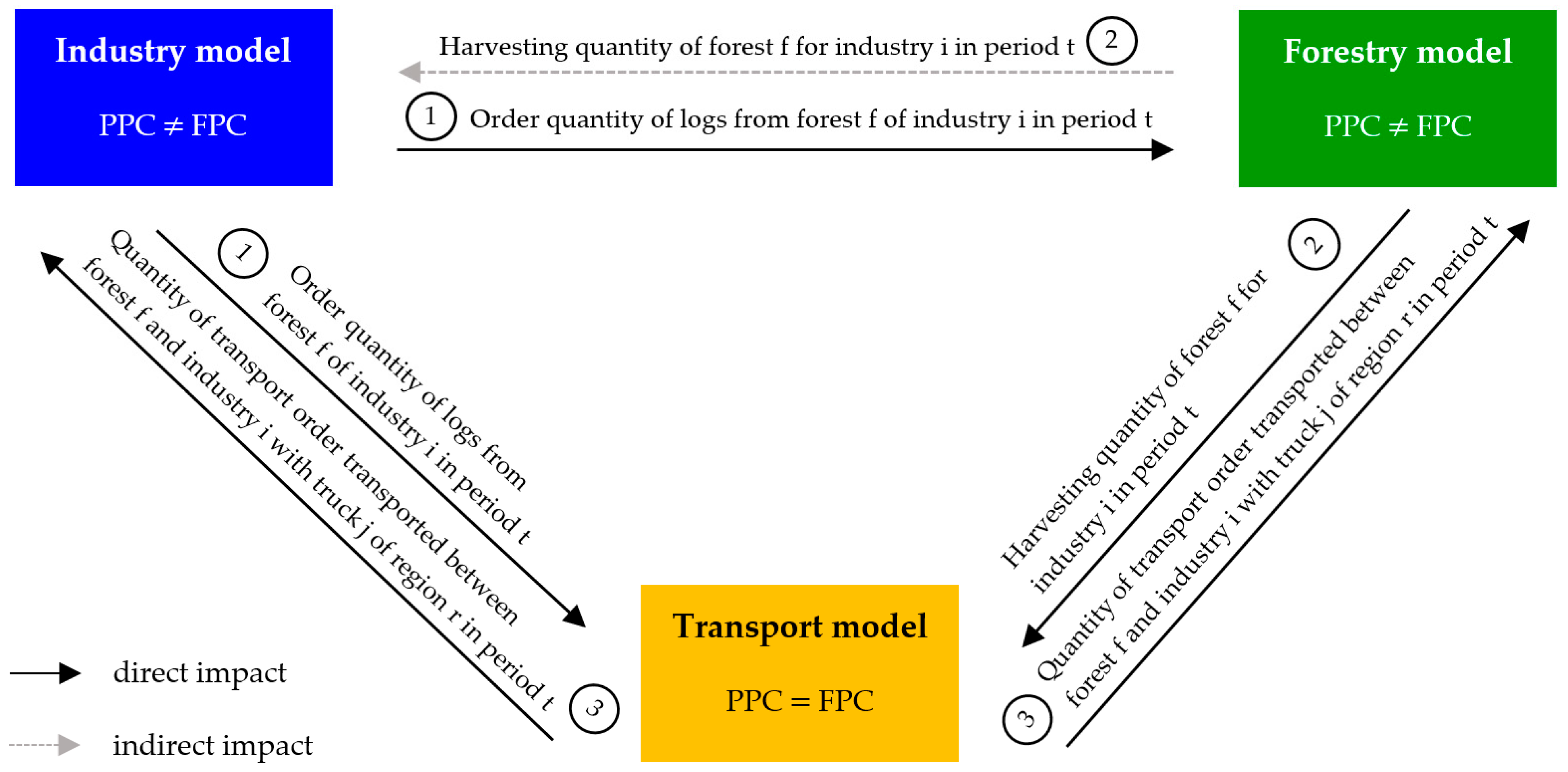
For each wood supply chain actor, a specific operational mixed-integer programming model is formulated. The models deal with short-term planning issues as the annual sourcing and harvesting plan of industries and forests was already defined and the total harvested round-wood of a forest is already assigned to a specific industry plant. Each actor individually makes his or her decisions considering their own interests on a weekly basis. The mathematical models are solved sequentially, starting with the industry model followed by the forestry model, and finally the transport model, as the solution of the preceding model(s) serves as input for the next one(s). The sequence of decisions is drawn in Figure 1, with arrows representing the decision variable of the corresponding actor.

Industries confronted with different demands for wood products determine optimal production plans and order quantities of wood. Forestry decides about bucking patterns and assortments per harvest site, harvesting quantity, and harvesting date to fulfill industrial demands. Trucking enterprises face a time window for each transport order, starting with the release date of piled logs at forests roadsides given by the forestry until the due date of transport order fulfillment given by the industries. Trucking enterprises have at least one week to perform a transport order, even if harvesting takes place at later periods than the requested order fulfillment time. Within these time windows, trucking enterprises have the flexibility to schedule transport orders smoothing workload and optimizing transport costs.

In the business-as-usual situation, all actors operate independently and make their decisions in an uncoordinated manner, optimizing their costs only under the given restrictions set by the decisions of predecessors and successors. Consequently, industries do not know the exact delivery time of logs and forestry does not know when the wood will be picked up at the moment of their decision-making. Therefore, the first result of the industry as well as of the forestry model corresponds to planned procurement costs (PPC). Final procurement costs (FPC) have to be calculated in a second step after all models have been solved. The procurement costs represent the combination of the actors’ objective functions, whose individual components are explained in the following descriptions of the industry, forestry, and transport model.

2.1. Industry Model

The objective function of the industry model (1) minimizes the sum of inventory holding, backlogging, fixed order, and penalty costs for violating safety stock and maximum inventory level over the whole T-period horizon. The planning problem of the industries representing an adapted lot-sizing problem can be defined as a selection of time when to achieve what quantity of logs from which forest.

Although the annual harvesting and sourcing plan assures that the total order quantity of one industry equals its demand for wood products over the total planning horizon (9), the delivered quantity does not always equal the ordered quantity and depends on the decisions of subsequent actors. It is assumed that the stock and backlog of logs at the beginning of the planning horizon is zero (2–5). Restrictions (6) and (7) represent the inventory balance restrictions of one industry for logs from forest enterprises and small-scale forests. On the customer side, industries are confronted with a demand for wood products that must be satisfied (8). As industries are dependent on continuous deliveries throughout the year, safety stocks (11) and maximum inventory levels (12) cause extra costs for external storage when exceeded (13–15), but mitigate predominated variability at the supply side. Restriction (16) relates the decision variable of log demand at forest enterprises with the general demand parameter. For the industry model, the indexes (

Table 1. Indexes of the industry model.

Term	Definition
$i=1\dots I$	Set of industries
$f=1\dots F$	Set of forests
$F=F^G{\displaystyle \cup }{F}^K$	Set of forests (forest enterprises and small-scale forests)
$F^G$	Set of forest enterprises
$F^K$	Set of small-scale forests
$t=1\dots T$	Set of time periods

), decision variables (

Table 2. Decision variables of the industry model.

Term	Definition
$I{I}_{i,t}^{G+}$	Quantity of logs from forest enterprises stored at industry $i$ at the end of time period $t$
$I{I}_{i,t}^{K+}$	Quantity of logs from small-scale forests stored at industry $i$ at the end of time period $t$
$I{I}_{i,t}^{G-}$	Quantity of logs from forest enterprises backlogged at industry $i$ at the end of time period $t$
$I{I}_{i,t}^{K-}$	Quantity of logs from small-scale forests backlogged at industry $i$ at the end of time period $t$
$y_{i,f,t}$	$\{\begin{array}{c}1 \mathrm{Industry} i \mathrm{orders} \mathrm{in} \mathrm{period} t \mathrm{from} \mathrm{forest} f \hfill \\ 0 \mathrm{Else} \hfill \end{array}$
${\sigma }_{i,t}^{min}$	$\{\begin{array}{c}1 \mathrm{Industry} i \mathrm{has} \mathrm{less} \mathrm{inventory} \mathrm{as} \mathrm{the} \mathrm{requested} \mathrm{safety} \mathrm{stock} \mathrm{in} \mathrm{period} t\hfill \\ 0 \mathrm{Else} \hfill \end{array}$
${\sigma }_{i,t}^{max}$	$\{\begin{array}{c}1 \mathrm{Industry} i \mathrm{surpasses} \mathrm{the} \mathrm{maximum} \mathrm{inventory} \mathrm{level} \mathrm{in} \mathrm{period} t\hfill \\ 0 \mathrm{Else} \hfill \end{array}$
$u_{i,t}^G$	Demand for logs of forest enterprises of industry $i$ in period $t$
$x_{i,f,t}$	Order quantity of industry i of logs from forest $f$ in period $t$
${\beth }_{i,t}^{max}$	Quantity which surpasses the maximum inventory level of industry $i$ in period $t$

), and parameters (

Table 3. Parameters of the industry model.

Term	Definition
$h_i$	Inventory holding costs of industry $i$
$h^{min}$	Penalty costs of violating the safety stock
$h^{max}$	Penalty costs per piece to surpass the maximum inventory level
$b_i^G$	Backlogging costs of logs from forest enterprises of industry $i$
$b_i^K$	Backlogging costs of logs from small-scale forests of industry $i$
${\omega }_i$	Fixed order costs of industry $i$
$u_{i,t}$	Total demand for logs of industry $i$ in period $t$
${\phi }_i^{G+}$	Initial inventory level of logs from forest enterprises at industry $i$
${\phi }_i^{K+}$	Initial inventory level of logs from small-scale forests at industry $i$
${\phi }_i^{G-}$	Initial level of backlog of logs from forest enterprises at industry $i$
${\phi }_i^{K-}$	Initial level of backlog of logs from small-scale forests at industry
$M_{i,f}$	Maximum order quantity of industry $i$ for logs from forest $f$ over total planning horizon
$I{I}_i^{max}$	Maximum inventory level of industry $i$
$I{I}_i^{min}$	Level of safety stock from industry $i$

) are defined as follows:

$$MIN={\displaystyle \sum }_{i\in I}{\displaystyle \sum }_{t\in T}\begin{array}{c}[\left(I{I}_{i,t}^{G+}+I{I}_{i,t}^{K+}\right)*h_i+I{I}_{i,t}^{G-}*b_i^G+I{I}_{i,t}^{K-}*b_i^K+{\displaystyle \sum _{f\in F}}{y}_{i,f,t}*{\omega }_i+\\ \left({\beth }_{i,t}^{max}-I{I}_i^{max}\right)*h^{max}+{\sigma }_{i,t}^{min}*h^{min}]\end{array}$$

(1)

$$I{I}_{i,0}^{G+}={\phi }_i^{G+} \forall i \in I$$

(2)

$$I{I}_{i,0}^{G-}={\phi }_i^{G-} \forall i \in I$$

(3)

$$I{I}_{i,0}^{K+}={\phi }_i^{K+} \forall i \in I$$

(4)

$$I{I}_{i,0}^{K-}={\phi }_i^{K-} \forall i \in I$$

(5)

$$I{I}_{i,t}^{G+}-I{I}_{i,t}^{G-}=I{I}_{i, t-1}^{G+}-I{I}_{i,t-1}^{G-}+{{\displaystyle \sum }}_{f\in F^G}{x}_{i,f,t}-u_{i,t}^G \forall i \in I, t \in T$$

(6)

$$I{I}_{i,t}^{K+}-I{I}_{i,t}^{K-}=I{I}_{i, t-1}^{K+}-I{I}_{i,t-1}^{K-}+{{\displaystyle \sum }}_{f\in F^K}{x}_{i,f,t}-(u_{i,t}-u_{i,t}^G) \forall i \in I, t \in T$$

(7)

$${{\displaystyle \sum }}_{t\in T}{{\displaystyle \sum }}_{f\in F}{x}_{i,f,t}={{\displaystyle \sum }}_{t\in T}{u}_{i,t} \forall i \in I$$

(8)

$${{\displaystyle \sum }}_{t\in T}{x}_{i,f,t}=M_{i,f} \forall i \in I, f\in F$$

(9)

$$x_{i,f,t}\le y_{i,f,t}*M_{i,f} \forall i \in I, t \in T, f\in F$$

(10)

$$I{I}_{i,t}^{G+}+I{I}_{i,t}^{K+}\ge I{I}_i^{min}-BigM*{\sigma }_{i,t}^{min} \forall i \in I, t \in T$$

(11)

$$I{I}_{i,t}^{G+}+I{I}_{i,t}^{K+}\le I{I}_i^{max}+BigM*{\sigma }_{i,t}^{max} \forall i \in I, t \in T$$

(12)

$${\beth }_{i,t}^{max}\le {\sigma }_{i,t}^{max}*BigM \forall i \in I, t \in T$$

(13)

$${\beth }_{i,t}^{max}\ge I{I}_{i,t}^{G+}+I{I}_{i,t}^{K+}-BigM*(1-{\sigma }_{i,t}^{max}) \forall i \in I, t \in T$$

(14)

$${\beth }_{i,t}^{max}\le I{I}_{i,t}^{G+}+I{I}_{i,t}^{K+}+BigM*(1-{\sigma }_{i,t}^{max}) \forall i \in I, t \in T$$

(15)

$$u_{i,t}^G\le u_{i,t} \forall i \in I, t \in T$$

(16)

$$I{I}_{i,t}^{G+}, I{I}_{i,t}^{K+}, I{I}_{i,t}^{G-}, I{I}_{i,t}^{K-}, x_{i,f,t}, u_{i,t}^{\prime G}, {\beth }_{i,t}^{max}\ge 0 \forall i \in I, t \in T, f\in F$$

(17)

$$y_{i,f,t}, {\sigma }_{i,t}^{min}, {\sigma }_{i,t}^{max}\in \left\{0,1\right\} \forall i \in I, t \in T, f\in F$$

(18)

2.2. Forestry Model

The objective function (19) of the forestry model minimizes fixed and variable harvesting costs, capital, and backlogging costs, extra costs arising through increasing inefficiency due to limited space at a stand, and the loss of profit through value downgrading of logs over the entire planning period. Confronted with the log demand of diverse industries ($x_{i,f,t}$), the planning problem of forestry starts with the decision of what quantity should be harvested at what stand in each period to fulfill the specific demand of industries (22) and (23).

Independent of the individual harvesting plan per stand, each stand is harvested completely over the considered time period, which is determined at the annual harvesting and sourcing plan (29). While no holding costs for stored logs must be paid, the forestry is confronted with capital costs as the raw material is not yet sold. The inventory balance constraints are formulated in (36). In case of backlogs, the forestry has to bear additional backlogging costs to ensure satisfying log demand (e.g., harvest in areas that were not initially planned, additional costs for hiring extra harvesting staff and resources, urgent transport relocating logs to intermediate stands that are permanently accessible). Inefficiency costs arise as forest road storage is limited and harvesting as well as transport operations are hindered if inventories exceed a specific level. This is reflected through maximum inventory levels and penalty costs, which are modeled through offsetting a lump sum in case of violation (37)–(39). Profit loss through value downgrading of round-wood arises if batches of logs are stored too long at a pile as timber quality decreases (e.g., through blue stain) resulting in a lower selling price. The calculation of value downgrading quantities of different assortments is modeled in restriction (40) and (41). Forestry has to decide optimal tree cutting directives to ensure fulfilling the industry demand of different assortments. The quantity of the lowest and most valuable part of a tree is limited (24) and used for satisfying sawlog demand. As sawlogs are potential substitutes for pulpwood, the total supply quantity of logs for paper mills can be expanded (25). For the industry model, the indexes (

Table 4. Indexes of the forestry model.

Term	Definition
$I=I^S\cup I^{P }$	Set of industries
$I^S$	Set of sawmills
$I^P$	Set of paper mills
$F=F^S\cup F^{P }$	Set of forests (forest enterprises and small-scale forests)
$t=1\dots T$	Set of time periods

), decision variables (

Table 5. Decision variables of the forestry model.

Term	Definition
$z_{f,t}$	$\{\begin{array}{c}1 \mathrm{Forest} f \mathrm{harvests} \mathrm{in} \mathrm{period} t\hfill \\ 0 \mathrm{Else}\hfill \end{array}$
$q_{f,t}$	Total harvesting quantity of forest $f$ in period $t$ composed of $q_{f,t}^S \mathrm{and} q_{f,t}^P$
$q_{i,f,t}$	Harvesting quantity of forest $f$ for industry $i$ in period $t$
$q_{f,t}^S$	Total sawlog harvesting quantity of forest $f$ in period $t$
$q_{f,t}^P$	Total pulpwood harvesting quantity of forest $f$ in period $t$
$I{F}_{i,f,t}^{+}$	Quantity of logs for industry $i$ at forest $f$ in period $t$
$I{F}_{i,f,t}^{-}$	Backlog quantity of logs for industry $i$ at forest $f$ in period $t$
$V_{i,f,t}^S$	Quantity of sawlogs for industry $i$ at forest $f$, which must be downgraded in period $t$
$V_{i,f,t}^P$	Quantity of pulpwood for industry $i$ at forest $f$, which must be downgraded in period $t$
${\beta }_{f,t}$	$\{\begin{array}{c}1 \mathrm{Storage} \mathrm{capacity} \mathrm{of} \mathrm{forest} f \mathrm{is} \mathrm{surpassed} \mathrm{in} \mathrm{period} t \hfill \\ 0 \mathrm{Else}\hfill \end{array}$
${\mu }_{f,t}$	Utilization of storage capacity of forest $f$ in period $t$
${\lambda }_{i,f,t}$	$\{\begin{array}{c}1 \mathrm{Forest} f \mathrm{has} \mathrm{a} \mathrm{backlog} \mathrm{for} \mathrm{the} \mathrm{demand} \mathrm{of} \mathrm{industry} i \mathrm{in} \mathrm{period} t \hfill \\ 0 \mathrm{Forest} f \mathrm{has} \mathrm{inventories} \mathrm{for} \mathrm{the} \mathrm{demand} \mathrm{of} \mathrm{industry} i \mathrm{in} \mathrm{period} t\hfill \end{array}$

), and parameters (

Table 6. Parameters of the forestry model.

Term	Definition
${\kappa }_f^{fix}$	Fixed harvesting costs of forest $f$
${\kappa }_f^{var}$	Variable harvesting costs/solid cubic meters of forest $f$
$b_f$	Backlogging costs of forest $f$
${\kappa }^{WS}$	Profit loss for downgraded sawlogs
${\kappa }^{WP}$	Profit loss for downgraded pulpwood
${\kappa }_f^{SLA}$	Lump sum costs at forest $f$ in case of surpassing capacity restriction
$C_f$	Maximum available harvesting quantity of forest $f$
$d_{i,f,t}$	Demand of industry $i$ for logs of forest $f$ in period $t$
$\alpha$	Share of sawlogs depending on bucking decision measured based on $C_f$
$I{F}_f^{max}$	Maximum inventory capacity of forest $f$
$q_f^{min}$	Minimum quantity for harvesting of forest $f$
${\varrho }_f$	Boundary of inventory capacity of forest $f$
$h_f$	Capital costs of forest $f$
WS/WP	Time when downgrading of sawlogs/pulpwood appears

) are defined as follows:

$$MIN={\displaystyle \sum }_{f\in F}{\displaystyle \sum }_{t\in T}[z_{f,t}*{\kappa }_f^{fix}+q_{f,t}*{\kappa }_f^{var}+{\displaystyle \sum }_{i\in I}I{F}_{i,f,t}^{+}*h_f+{\beta }_{f,t}*{\kappa }_f^{SLA}+{\displaystyle \sum }_{i\in I}I{F}_{i,f,t}^{-}*b_f+V_{i,f,t}^S*{\kappa }^{WS}+V_{i,f,t}^P*{\kappa }^{WP}]$$

(19)

$$q_{f,t}\le z_{f,t}*C_f \forall f\in F,t\in T$$

(20)

$$q_{f,t}\ge z_{f,t}*q_f^{min} \forall f\in F,t\in T$$

(21)

$${{\displaystyle \sum }}_{t\in T}{q}_{f,t}^S={{\displaystyle \sum }}_{t\in T}{{\displaystyle \sum }}_{i\in I^S}{d}_{i,f,t} \forall f\in F$$

(22)

$${{\displaystyle \sum }}_{t\in T}{q}_{f,t}^P={{\displaystyle \sum }}_{t\in T}{{\displaystyle \sum }}_{i\in I^P}{d}_{i,f,t} \forall f\in F$$

(23)

$${{\displaystyle \sum }}_{t\in T}{q}_{f,t}^S\le C_f*\alpha \forall f\in F$$

(24)

$${{\displaystyle \sum }}_{t\in T}{q}_{f,t}^P\le C_f-{{\displaystyle \sum }}_{t\in T}{q}_{f,t}^S \forall f\in F$$

(25)

$$q_{f,t}=q_{f,t}^P+q_{f,t}^S \forall f\in F,t\in T$$

(26)

$$q_{f,t}^S\le \alpha *q_{f,t} \forall f\in F,t\in T$$

(27)

$$q_{f,t}^P\ge q_{f,t}*(1-\alpha ) \forall f\in F,t\in T$$

(28)

$${{\displaystyle \sum }}_{t\in T}{q}_{f,t}=C_f \forall f\in F$$

(29)

$${{\displaystyle \sum }}_{i\in I^S}{q}_{i,f,t}=q_{f,t}^S \forall f\in F,t\in T$$

(30)

$${{\displaystyle \sum }}_{i\in I^P}{q}_{i,f,t}=q_{f,t}^P \forall f\in F,t\in T$$

(31)

$$I{F}_{i,f,0}^{+}=0 \forall i \in I, f \in F$$

(32)

$$I{F}_{i,f,0}^{-}=0 \forall i \in I, f \in F$$

(33)

$$I{F}_{i,f,t}^{+}\le 0+BigM*(1-{\lambda }_{i,f,t}) \forall i \in I, f\in F,t\in T$$

(34)

$$I{F}_{i,f,t}^{-}\le 0+BigM*{\lambda }_{i,f,t} \forall i \in I, f\in F,t\in T$$

(35)

$$I{F}_{i,f,t}^{+}-I{F}_{i,f,t}^{-}=I{F}_{i,f,t-1}^{+}-I{F}_{i,f,t-1}^{-}+q_{i,f,t}-d_{i,f,t} \forall i \in I, f\in F,t\in T$$

(36)

$${{\displaystyle \sum }}_{i\in I}I{F}_{i,f,t}^{+}\le I{F}_f^{max} \forall f\in F,t\in T$$

(37)

$$\frac{{{\displaystyle \sum }}_{i\in I}I{F}_{i,f,t}^{+}}{I{F}_f^{max}}={\mu }_{f,t} \forall f\in F,t\in T$$

(38)

$${\mu }_{f,t}\le {\varrho }_f+\left(1-{\varrho }_f\right)*{\beta }_{f,t} \forall f\in F,t\in T$$

(39)

$$V_{i,f,t}^S\ge I{F}_{i,f,t-1}^{+}-I{F}_{i,f,t-1}^{-}+q_{i,f,t}-{{\displaystyle \sum }}_{n=t}^{t+WS}{d}_{i,f,n}-V_{i,f, t-1}^S \forall i\in I^S,f\in F,t\in T$$

(40)

$$V_{i,f,t}^P\ge I{F}_{i,f,t-1}^{+}-I{F}_{i,f,t-1}^{-}+q_{i,f,t}-{{\displaystyle \sum }}_{n=t}^{t+WP}{d}_{i,f,n}-V_{i,f, t-1}^P \forall i\in I^P,f\in F,t\in T$$

(41)

$$V_{i,f, 0}^S=0 \forall i\in I, f\in F$$

(42)

$$V_{i,f, 0}^P=0 \forall i\in I, f\in F$$

(43)

$$q_{f,t}, q_{i,f,t}, I{F}_{i,f,t}^{+}, I{F}_{i,f,t}^{-}, V_{i,f,t}^S, V_{i,f,t}^P, q_{f,t}^S, q_{f,t}^P, {\mu }_{f,t}\ge 0 \forall i \in I, f\in F,t\in T$$

(44)

$$z_{f,t}, {\beta }_{f,t}, {\lambda }_{i,f,t}\in \left\{0,1\right\} \forall i\in I, f\in F,t\in T$$

(45)

2.3. Transport Model

The objective function of the transport model (46) maximizes the profit attained from transporting logs from different forest sites to industry locations in their transport region minus total transport costs consisting of a variable and a fixed cost. The planning problem of trucking enterprises is to decide the optimal schedule of transport orders with respect to possible time slots of orders, legal restrictions in regard to transport payload per truck (50) and driving time per truck driver (51), and maximum inventory levels of industries (56–58), with the goal to achieve a smooth workload.

As industries and forestry can order and harvest multiple times, the trucking enterprise is free to combine quantities of different transport orders, but all transport orders must be fulfilled (47). Trucking enterprises are responsible for a specific geographical area because, in mountainous regions, regional truck drivers are needed to find pick-up points despite lacking GPS support. Restriction (48) ensures that a trucking enterprise fulfills orders falling within their remit. A transport order is defined for each order of one industry at one forest enterprise, including a specific due date. The release date of a transport order is defined by the harvesting time since transport can start as soon as the corresponding logs are harvested. The parameter $v_{i,f,a,t}$ defines in which period a transport order can be fulfilled. Aside from defined potential larger time slots, a trucking enterprise has at least one period for executing the transport order. The time span of order settlement is modeled in (49). Imbalances in daily workloads lead to organizational problems and higher costs, therefore trucking enterprises try to distribute transport orders equally over the periods (52)–(54). Even though trucking enterprises are confronted with high costs for overtime as well as organizing additional external trucks and equipment to cover high workload in peak times, they are forced to pay overhead costs with no related profit in times of capacity underutilization. For the transport model, the indexes (

Table 7. Indexes of the transport model.

Term	Definition
$i=1\dots I$	Set of industries
$f=1\dots F$	Set of forests
$a=1\dots A$	Set of transport orders
$t=1\dots T$	Set of time periods
$r=1\dots R$	Set of transport regions
$j=1\dots J$	Set of trucks

), decision variables (

Table 8. Decision variables of the transport model.

Term	Definition
$m_{i,f,a,j,t,r}$	Quantity of transport order $a$, which is transported between forest $f$ and industry $i$ with truck $j$ of region $r$ in period
$l_{j,t,r}$	$\{\begin{array}{c}1 \mathrm{Truck} j \mathrm{of} \mathrm{region} r \mathrm{is} \mathrm{used} \mathrm{in} \mathrm{period} t \hfill \\ 0 \mathrm{Else} \hfill \end{array}$
${\rho }_{t, r}$	Positive deviation from average number of trucks used in region $r$ in period $t$
${\eta }_{t,r}$	Deviation from average number of trucks used in region $r$ in period $t$
${\mathsf{{\rm Y}}}_r$	Average number of trucks used in region $r$
${\varphi }_{i,f,j,t,r}$	Minimum number of transports from forest $f$ to industry $i$, not violating the admissible gross vehicle weight of truck $j$ of region $r$ in period $t$
$I{I}_{i,t}$	Total quantity of logs stored at industry $i$ at the end of time period $t$

), and parameters (

Table 9. Parameters of the transport model.

Term	Definition
$P_{i,f}$	Price of transporting a log from forest $f$ to industry $i$
${\tau }_{i,f}$	Variable costs of driving once the route between forest $f$ and industry $i$
${\tau }_r^{Lfix}$	Fixed costs per used truck in region $r$
${\psi }^{\eta }$	Additional costs to pay in case the number of trucks used negatively deviates from the average number of trucks used over the entire time horizon
${\psi }^{\rho }$	Additional costs to pay in case the number of trucks used positively deviates from the average number of trucks used over the entire time horizon
$v_{i,f,a,t}$	$\{\begin{array}{c}1 \mathrm{Order} a \mathrm{between} \mathrm{forest} f \mathrm{and} \mathrm{industry} i \mathrm{can} \mathrm{be} \mathrm{fullfilled} \mathrm{in} \mathrm{period} t \mathrm{with} \mathrm{respect} \mathrm{to} \mathrm{release} \mathrm{and} \mathrm{due} \mathrm{date}\hfill \\ 0 \mathrm{Else} \hfill \end{array}$
${\delta }_{i,f}$	Driving time from forest $f$ to industry $i$
$\varsigma$	Maximum legal driving time of a truck driver
${\aleph }_{i,f,r}$	$\{\begin{array}{c}1 \mathrm{Region} r \mathrm{is} \mathrm{respsonible} \mathrm{for} \mathrm{the} \mathrm{transport}\hfill \\ \mathrm{route} \mathrm{between} \mathrm{forest} f \mathrm{and} \mathrm{industry} i\\ 0 \mathrm{Else} \hfill \end{array}$
${\varpi }_{i,f,a}$	Weight of logs of transport order $a$ of forest-industry pair
$\beth$	Maximum legal truck payload
$u_{i,t}$	Demand of industry $i$ in period
$I{I}_i^{max}$	Maximum inventory level of industry $i$
${\phi }_i$	Initial inventory level of industry $i$

) are defined as follows:

$$MAX={\displaystyle \sum }_{r\in R}{\displaystyle \sum }_{t\in T}\left[{\displaystyle \sum }_{j\in J}{\displaystyle \sum }_{i\in I}{\displaystyle \sum }_{f\in F}{\displaystyle \sum }_{a\in A}(\underset{i,f}{P} *\underset{i,f,a,j,t,r}{m})-{\displaystyle \sum }_{i\in I}{\displaystyle \sum }_{f\in F}{\displaystyle \sum }_{j\in J}{\varphi }_{i,f,j,t,r}*{\tau }_{i,f}-{\displaystyle \sum }_{j\in J} l_{j,t,r}*{\tau }_r^{Lfix}-{\eta }_{t,r}*{\psi }^{\eta }-{\rho }_{t, r}*{\psi }^{\rho }\right]$$

(46)

$${{\displaystyle \sum }}_{r\in R}{{\displaystyle \sum }}_{t\in T}{{\displaystyle \sum }}_{j\in J}{m}_{i,f,a,j,t,r}={\varpi }_{i,f,a} \forall i\in I,f\in F,a\in A$$

(47)

$${{\displaystyle \sum }}_{t\in T}{{\displaystyle \sum }}_{j\in J}{{\displaystyle \sum }}_{a\in A}{m}_{i,f,a,j,t,r}\le {\aleph }_{i,f,r}*BigM \forall i\in I,f\in F, r\in R$$

(48)

$${{\displaystyle \sum }}_{r\in R}{{\displaystyle \sum }}_{j\in J}{m}_{i,f,a,j,t,r}\le v_{i,f,a,t}*{\varpi }_{i,f,a} \forall i\in I,f\in F,a\in A, t\in T$$

(49)

$${{\displaystyle \sum }}_{a\in A}{m}_{i,f,a,j,t,r}\le \beth *{\varphi }_{i,f,j,t,r} \forall i\in I,f\in F,j\in J,t\in T,r\in R$$

(50)

$${{\displaystyle \sum }}_{i\in I}{{\displaystyle \sum }}_{f\in F}{\varphi }_{i,f,j,t,r}*{\delta }_{i,f}\le \varsigma *l_{j,t,r} \forall j\in J,t\in T,r\in R$$

(51)

$${\mathsf{{\rm Y}}}_r=\frac{{{\displaystyle \sum }}_{t\in T}{{\displaystyle \sum }}_{j\in J}{l}_{j,t,r}}{T} \forall r\in R$$

(52)

$${\eta }_{t,r}\ge {\mathsf{{\rm Y}}}_r-{{\displaystyle \sum }}_{j\in J}{l}_{j,t,r} \forall t\in T,r\in R$$

(53)

$${\rho }_{t, r}\ge {{\displaystyle \sum }}_{j\in J}{l}_{j,t,r}-{\mathsf{{\rm Y}}}_r \forall t\in T,r\in R$$

(54)

$${{\displaystyle \sum }}_{i\in I}{{\displaystyle \sum }}_{f\in F}{{\displaystyle \sum }}_{a\in A}{m}_{i,f,a,j,t,r}\le l_{j,t,r}*BigM \forall j\in J,t\in T,r\in R$$

(55)

$$I{I}_{i,t}=I{I}_{i,t-1}+{{\displaystyle \sum }}_{f\in F}{{\displaystyle \sum }}_{a\in A}{{\displaystyle \sum }}_{j\in J}{{\displaystyle \sum }}_{r\in R}{m}_{i,f,a,j,t,r}-u_{i,t} \forall t\in T,i\in I$$

(56)

$$I{I}_{i,0}={\phi }_i \forall i\in I$$

(57)

$$I{I}_{i,t}\le I{I}_i^{max} \forall t\in T,i\in I$$

(58)

$${\eta }_{t,r}, {\rho }_{t, r},{ \mathsf{{\rm Y}}}_r, {\varphi }_{i,f,j,t,r},m_{i,f,a,j,t,r}, I{I}_{i,t}\ge 0 \forall i\in I,f\in F,a\in A,j\in J,t\in T,r\in R$$

(59)

$$l_{j,t,r}\in \left\{0,1\right\} \forall t\in T,r\in R, j\in J$$

(60)

3. Results

Models, strategies, and scenarios were parameterized based on case study data of the Austrian provinces Carinthia and Styria. The demand network for the industry model covers three paper mills and one sawmill. The supply network includes 35 forests divided into 20 forest enterprises with more than 200 hectares of forest area and 15 small-scale forests with a forest area of less than 200 hectares. For transport, data from 11 regional trucking enterprises were collected. From the data set, it is ensured that both the total transport capacity is high enough to fulfill all transport orders and the combined transport capacity is greater than timber demand. Since data were collected from competing companies including internal and sensitive information, data sets cannot be published.

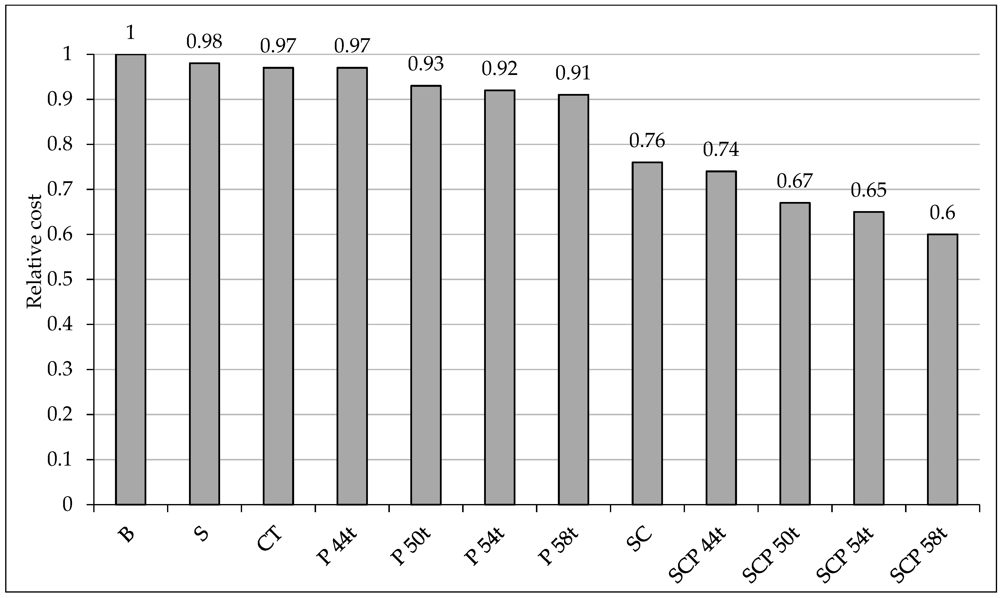
Strategies and scenarios were calculated with AMPL Version: 3.5.0.201802211250. With the data set from the case study region, approximately five million decision variables and 170,000 constraints were necessary for the business-as-usual case (base strategy). Even with the included pre-optimization of AMPL, which cuts non-binding constraints and ignores unnecessary decision variables, the sheer size of the problem leads to calculation times of several hours per model. To reduce calculation time, an accuracy tolerance (i.e., the difference between the current ILP solution and the corresponding LP-relaxation) of a maximum of 10% was accepted. The procurement costs, as well as the coefficients of variation, were set in relation to the base strategy in order to provide a benchmark and summarized in

Table 10. Relative procurement costs and coefficient of variation of the strategies and scenarios.

Strategy	Scenario	Cost	Coefficient of Variation in %
			COQ	CHQ	CTQ
Base		1	16	37	8
Coordinated Transport		0.97	16	37	22
Payload	44 t	0.97	16	37	14
	50 t	0.93	16	37	12
	54 t	0.92	16	37	11
	58 t	0.91	16	37	19
Supply Chain	IFT	0.76	9	38	9
	I	1.32	10	39	10
	F	0.93	22	51	22
	T	2.41	15	49	15
Supply Chain Payload	44 t	0.74	23	50	23
	50 t	0.67	15	54	15
	54 t	0.65	9	40	9
	58 t	0.60	13	54	13
Satellite Stockyard		0.98	14	58	33

Coefficient of variation in %: COQ = coefficient of order quantity, CHQ = coefficient of harvest quantity, CTQ = coefficient of transport quantity; scenario: IFT = industry forestry transport, I = industry, F = forestry, T = transport.

and Figure 2.

3.1. Base (B) Strategy

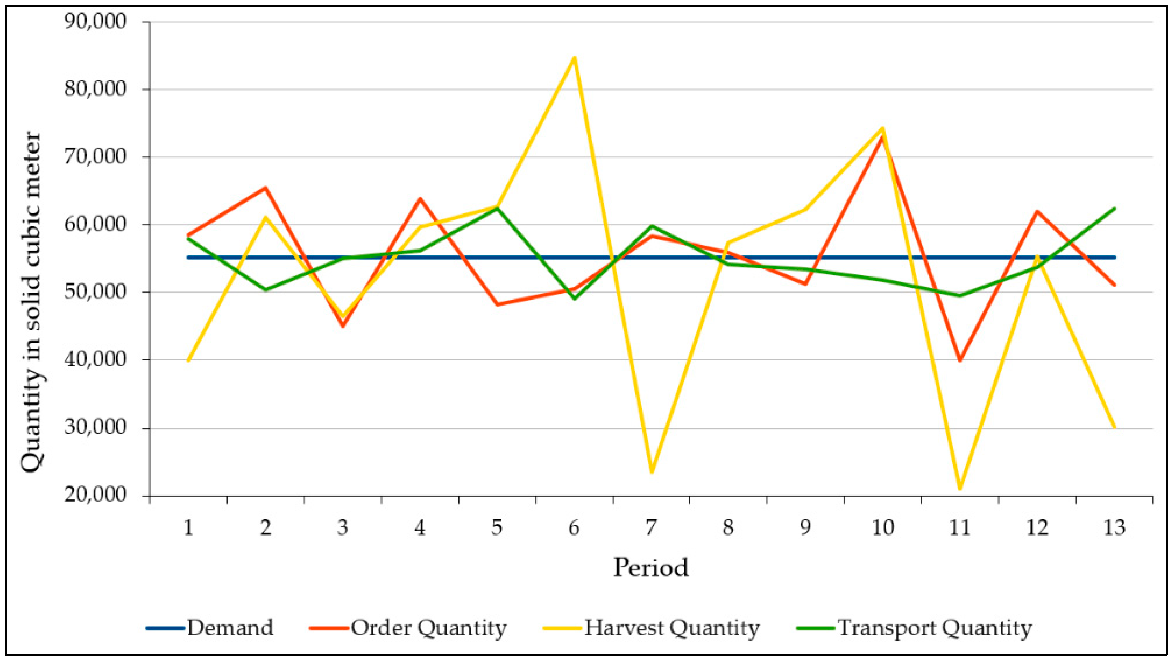
Looking at the material flow, industries are confronted with a consistent demand for wood products. The industry starts with the batch building leading to a coefficient of variation of the order quantity (COQ) of 16% for the industry. Afterward, forestry batches harvest operations even more resulting in a coefficient of variation of the harvest quantity (CHQ) of 37%. This increasing fluctuation along the supply chain is well known as the bullwhip effect as shown in Figure 3.

3.2. Coordinated Transport (CT) Strategy

In this strategy, central planning is simulated to examine the advantages of a coordinated transport system and respective potential procurement cost savings. To model this case, capacities and locations of all transport agents were combined, resulting in one transport region. The industry and forestry models remain unchanged to the base strategy. Coordinated transport by a central planning unit results in cost savings of 3%, although the overall transport fluctuation measured by the coefficient of variation of the transport quantity (CTQ) increases from 8% to 22%, whereas COQ and CHQ remain at 16% and 37%, respectively.

3.3. Payload (P) Strategy

The payload strategy evaluates procurement cost-saving potentials through the increase of the maximum gross vehicle weight to 44, 50, 54, and 58 t, respectively. In Austria, the general legal gross vehicle weight for trucks is 40 t, but an exemption exists for log transport on self-loading trucks. A gross vehicle weight of 44 t is allowed if the destination is within 100 km of the harvest site. Moreover, after natural disasters such as storm damages or bark beetle infestations, the gross vehicle weight limit can be raised up to 50 t by provincial governments.

An increase of gross vehicle weight to 44, 50, 54, and 58 t can save up to 3%, 7%, 8%, and 9%, respectively. The biggest cost-saving step is already achieved by 50 t. All cost savings can be directly allocated to the transport model since there are no changes in the industry and forestry model. The COQ and CHQ remain unchanged from the base strategy since the increase of the maximal vehicle weight of trucks only concerns the transport model. The CTQ changes to 14% (44 t), 12% (50 t), 11% (54 t), and 19% (58 t).

3.4. Supply Chain (SC) Strategy

The third cost-saving strategy analyzes the effects of an integrated supply chain. In the supply chain strategy, a centralized planning unit is simulated, where all decisions regarding the vertical supply chain are made simultaneously. Therefore, order quantity, harvest quantity, and transport quantity are perfectly synchronized with each other. To simulate an integrated timber supply chain, the three models were combined into one supply chain model. One change that had to be made was to flip the transport model from a maximization problem to a minimization problem, which was achieved by multiplying all functions of the transport model by minus one. For the supply chain objective function, the three objective functions were combined into a single objective function subjected to all constraints of the three models. The order quantity equals the transport quantity because of the coordination of the entire supply chain. Therefore, the order quantity decision variable and the transport quantity decision variable were combined into one decision variable that serves both purposes. The underlying constraints and objective function were changed to the new decision variable.

The impact of a shift in decision power between the different supply chain actors is illustrated by calculating the supply chain model in four scenarios. In the first scenario “industry forestry transport” (IFT), the decision power is equally distributed between the three actors. Every decision made is considered best for the integrated supply chain. For the other scenarios “industry” (I), “forestry” (F), and “transport” (T), all supply chain decisions are up to one actor (i.e., either I, F, or T) aiming to minimize their own costs without any regard to the other two actors. Through these scenarios, essential indications of power shifts within the SC can be attained. If the central planning unit prioritizes just one actor, it results in a critical worsening. If industry or transport is favored, procurement costs increase by 32% and 141%, respectively. Although prioritizing the forestry reduces costs by 7%, it still diminishes potential cost savings of the IFT scenario, as the IFT scenario saves up to 24% of the costs compared to the base strategy. All COQ and CTQ are identical to each other since the coordination is perfectly synchronized in the SC. The corresponding coefficients for IFT, I, F, and T are 9%, 10%, 22%, and 15%, respectively. The CHQ of the IFT, I, F, and T case are 38%, 39%, 51%, and 49%, respectively.

3.5. Supply Chain Payload (SCP) Strategy

In this strategy, a payload increase is implemented into the IFT scenario of the supply chain strategy to examine synergy and enforcing effects. A payload increase to 44, 50, 54, and 58 t results in procurement cost savings of 26%, 33%, 35%, and 40% compared to the base strategy, respectively. As in the SC strategy, COQ and CTQ are also equal in the SCP strategy. In the 44 t SCP, they are both 23% and CHQ is 50%. For the SCP 50 t, the COQ and CTQ are 15% and the CHQ is 54%. In the SCP 54 t case, the COQ and CTQ are 9% and the CHQ is 40%. For the SCP 58 t, the COQ and CTQ are 13% and the CHQ is 54%

3.6. Satellite Stockyard (S) Strategy

In this strategy, the base case model is extended by a stockyard allocated between forestry and industry sites, to take into account that storage on plant sites is limited and expensive. The satellite stockyard was modeled as a separate inventory where every route to and from the satellite stockyard had specific additional transportation costs. The holding costs for the satellite stockyard can be adjusted separately. At the stockyard, no quality loss of the stored timber was assumed. Transport from the stockyard to industries is carried out with semitrailer trucks that have a 6 t higher payload than a forest crane truck.

Introducing a satellite stockyard to the supply chain saves up to 2% procurement costs. Forestry operations take advantage of the satellite storage to cluster harvests, which can be observed through increased batch sizes and by the CHQ, which rose to 58%, the highest value in all strategies.

4. Discussion

The tremendous positive impacts of supply chain coordination and integration have already been observed in several articles. Accordingly, an integrated supply chain model was formulated to evaluate the potential of internal pricing as a mechanism to align forest harvest decisions and industrial production planning [19]. Others [20] compared the performance of a coordinated supply chain versus a supply chain, where business units set their decisions about operations unilaterally in a two-stage approach, by using the mean of the net present value. Moreover, it was shown by a linear programming model [22] that the integration of harvesting and production planning decisions simultaneously improves net revenue and ecosystem conservation compared to a decoupled supply chain strategy.

The presented models have in common with existing linear programming models of the wood supply chain [15,16,17] that the availability of logs is assumed to be already assigned in the long term. Each forest has a predetermined supply of logs, which cannot be succeeded. The presented model, and others [16,17] model restrictions about maximal sourcing volume of logs to introduce this assumption. Nevertheless, the presented model formulates the decision problem of forestry in more detail, clearly pointing out the interests and market power of forestry. Forestry can decide about bucking patterns and optimal harvesting times to fulfill industry orders. Contrary, in other wood supply chain models [15,16,17] the available quantity of logs is just a side constraint to consider. The focus of coordination lies in industries. Industries decide the optimal production and distribution plan for producing wood products and satisfying customer demand. They can freely decide when to procure the logs for production. Forestry has no market power to influence this decision. The transport smoothing and transport costs savings by reducing the required equipment and combining routes in the presented model are similarly modeled as in [11], which also consider forestry constraints as outlined in [8], even though saving costs is the main objective. In addition to a simplified production and demand formulation in the presented model, material flows between industries (e.g., from sawmills to pulp mills), the energy industry as a third member on the industry side as mentioned in the formulation of [19], additional procurement streams like recycled paper [23], and different transportation modes (i.e., ship, train, truck) [17] are not included. Contrary to the formulation of wood supply chain models considering industry and transport [11], or industry and forestry [20] as cooperating actors, the presented model denotes the decision situation of all participating forestry, transport, and industry actors of the wood supply chain in detail.

The results of this study focus on strategy and scenario analysis based on the presented mixed-integer programming models for forestry, round-wood transport, and wood-based industry to emphasize relative procurement cost-saving potential. Variability in order, delivery, and harvest volumes of the different strategies is not critical per se, especially for wood harvest volumes, but coordinating the supply chain improves the balance between transport capacity utilization and industry demand.

Since there are primarily small trucking enterprises handling only a small truck fleet in Austria, optimization and smoothing of every trucking enterprise individually might limit the cost-saving potential of timber transport. Consequently, the coordinated transport strategy combines all transport resources to benefit from economies of scale. In the CT strategy, the increase of the CTQ is acceptable since cost savings are achieved by combining transport capacities and benefit from shared resources. Wood bartering was discussed as a potential coordination method to share the profits arising through coordination by [33]. For Swedish case studies, cost-saving potentials were reported using back haulage routes (7%) and wood barter (5%) [34] as well as optimized truck route scheduling with a saving potential ranging from 5 to 30% [35]. Based on case study data from southern Sweden, collaboration in transportation planning saves up to 14% transportation costs and 20% emissions from the trucks [33]. Applying MILP-model optimizing transportation of energy wood to several plants, cooperation proved to result in 23% lower transport costs than through competition [36]. A transport costs saving potential of 2% was reported when optimization model results were compared to manual planning in a related Austrian case study region [37]. Although the positive effect of coordinated transport was reported, cost savings in relation to transport costs only accounted for part of the procurement costs. The reported 3% cost savings in this study, which can be directly allocated to transport coordination, are in relation to the total procurement costs.

Through payload increase, a linear decrease in costs is achieved, which was expected from an optimization standpoint. The considered gross payloads for Australian (i.e., 42.5, 62.5, 79 t) [32] and Finish (i.e., 68, 76, and 84 t) [30,31] conditions illustrate the comparatively low limits in Austria, resulting in the conservative scenario design for 44, 50, 54, and 58 t, which hinders direct comparisons. Nevertheless, savings by increasing the legal gross payloads were reported for Austrian condition, where an increase from 44 t to 50 t reduced the number of self-loading trucks in a multi-echelon unimodal wood supply chain cutting transport costs by 6–11% [26], depending on the transport distance and maximal terminal capacity utilization. This compares to a 4% procurement cost-cutting for a similar payload increase in the presented P strategy. For Finish conditions, comparable ranges of cost reduction by increased gross vehicle weights from 68 t to 76 t (i.e., +12% payload) and to 84 t (i.e., +24% payload) result in savings of trucking costs of up to 3% and 9%, respectively. In the presented payload strategy in this study, an increase of 10% and 25% payload results in 3% and 7% procurement cost reduction, respectively. Therefore, the payload effect on cost reduction shows for both countries a similar range even though differing methods had been applied (i.e., Agent-based Simulation for Finland and ILP for Austria).

In a case study of an integrated Swedish supply chain [38] including three pulp mills and ten domestic harvest areas focusing on transportation, storage, and production plan costs, potential savings of between 5 and 10% were shown when optimization model results were compared to manual planning. In the presented results based on Austrian case study data, a procurement cost-saving potential of up to 24% (SC) in an integrated supply chain was observed. Cooperation in Austrian wood supply chains is underdeveloped, resulting in a higher improvement potential compared to the Swedish cases. For the cost savings of the IFT scenario in the SC strategy, the driving force seems to be the perfect coordination between industry and transport quantity that can be observed by the COQ and CTQ value, which are equal in all cases with an integrated supply chain. The combination of increased payload and equally distributed decision power (IFT scenario) in the SCP strategy synergize perfectly. The steady increase of payload seamlessly works in the SCP and reinforces cost savings.

The satellite stockyard reduces risk to some extent as industry reduces internal stocks and increases order frequency, while forestry increases harvest quantity since the risk of quality depreciation is reduced. Furthermore, interim storage decouples wood harvesting volumes from orders but increases transport flexibility leading to cost savings. The presented model did not consider that logs stored at a stockyard naturally dry and more volume can be transported at the same truck payload, which reduces transportation costs by about 6% [25]. In addition, optimizing of terminal site location was not considered in this study, but has been covered by others [24].

5. Conclusions

The main contribution of this study is in providing a benchmark of wood procurement cost-saving strategies, comparing for the first time the relative impact of coordinated transport, higher truck payloads, integrated supply chain, integrated supply chain combined with higher truck payloads and satellite stockyards within a single case study setting. Coordination of transport planning and introducing interim storage provides the potential to reduce procurement costs, but increasing legal payload has a stronger impact. If industry or transport can coordinate the wood supply chain according to their specific goals, procurement costs considerably increase, whereas coordination from a forestry viewpoint leads to cost savings.

Coordination of the wood supply chain from an overall planning perspective gains tremendous cost savings, but also requires the commitment of all involved actors. Experiences from workshops accompanying this study indicate that wood supply chain managers prefer those strategies where the implementations are more in their control, even though they have a less positive impact on costs. Wood supply chain integration for Central European circumstances seems to be feasible only for a limited consortium of a few companies, for example, restricted to a wood-buying syndicate supplying several industry plants or a few large forest enterprises, especially as both groups are commonly steering wood transport on their own. The main managerial implications of this study lie in enhancing lobbying for increasing legal payload, deepening cooperation, and improving coordination with potent supply chain partners in order to reduce wood procurement costs.

The results for the different procurement cost-saving strategies fit well to reported findings of other studies, therefore it can be assumed that the presented models do well in representing both the wood supply chain and effects of the most relevant procurement cost-saving strategies. Limitations of the presented models, providing future research potential, are the reduction of the complexity of the wood supply chain by omitting seasonal supply risks with an impact on supply security and procurement costs such as spring thaw, heavy snowfall, or rainy periods delaying transport and harvest activities. The decision behavior of supply chain actors was unified, even though conflicting goals may occur due to a large number of forest enterprises and private small-scale forest owners resulting in different priorities. Further research on the challenging task of implementing integrated supply chains is needed using the opportunities of digitalization to realize cost savings potential by deepening cooperation and intensifying information exchange.

References

- Rönnqvist, M. Optimization in forestry. Math. Program. 2003, 97, 267–284. [Google Scholar] [CrossRef]
- D’Amours, S.; Rönnqvist, M.; Weintraub, A. Using Operational Research for Supply Chain Planning in the Forest Products Industry. INFOR Inf. Syst. Oper. Res. 2008, 46, 265–281. [Google Scholar] [CrossRef]
- Weintraub, A.; Romero, C.; Bjorndal, T.; Epstein, R.; Miranda, J. Handbook of Operations Research in Natural Resources, Forestry, International Series in Operations Research and Management Science; Springer: Berlin/Heidelberg, Germany, 2007; pp. 315–525. [Google Scholar]
- Acuna, M. Timber and biomass transport optimization: A Review of Planning Issues, Solution Techniques and Decision Support Tools. Croat. J. For. Eng. 2017, 38, 279–290. [Google Scholar]
- Acuna, M.; Sessions, J.; Zamora, R.; Boston, K.; Brown, M.; Ghaffariyan, M.R. Methods to Manage and Optimize Forest Biomass Supply Chains: A Review. Curr. For. Rep. 2019, 5, 124–141. [Google Scholar] [CrossRef]
- Väätäinen, K.; Anttila, P.; Eliasson, L.; Enström, J.; Laitila, J.; Prinz, R.; Routa, J. Roundwood and Biomass Logistics in Finland and Sweden. Croat. J. For. Eng. 2020, 42, 39–61. [Google Scholar] [CrossRef]
- Kogler, C.; Rauch, P. Discrete Event Simulation of Multimodal and Unimodal Transportation in the Wood Supply Chain: A Literature Review. Silva Fenn. 2018, 52, 29. [Google Scholar] [CrossRef]
- Karanta, I.; Jokinen, O.; Mikkola, T.; Savola, J.; Bounsaythip, C. Requirements for a Vehicle Routing and Scheduling System in Timber Transport. In Logistics in the forest sector, Proceedings of the 1st World Symposium on Logistics in the Forest Sector, Helsinki, Finland, 15–16 May 2000; Sjöström, K., Ed.; Timber Logistics Club: Helsinki, Finland, 2000; pp. 235–250. [Google Scholar]
- Palmgren, M.; Rönnqvist, M.; Värbrand, P. A Solution Approach for Log Truck Scheduling based on Composite Pricing and Branch and Bound. Int. Trans. Oper. Res. 2003, 10, 433–447. [Google Scholar] [CrossRef]
- Carlsson, D.; Rönnqvist, M. Backhauling in Forest Transportation: Models, Methods, and Practical Usage. Can. J. For. Res. 2007, 37, 2612–2623. [Google Scholar] [CrossRef]
- Hirsch, P.; Gronalt, M. The Timber Transport Order Smoothing Problem as Part of the Three-Stage Planning Approach for Round Timber Transport. J. Appl. Oper. Res. 2013, 5, 70–81. [Google Scholar]
- Hirsch, P. Minimizing Empty Truck Loads in Round Timber Transport with Tabu Search Strategies. Int. J. Inf. Syst. Supply Chain Manag. 2011, 4, 15–41. [Google Scholar] [CrossRef] [Green Version]
- Marques, A.F.; Rönnqvist, M.; D’Amours, S.; Weintraub, A.; Gonçalves, J.; Borges, J.G.; Flisberg, P. Solving the Raw Materials Reception Problem Using Revenue Management Principles: An Application to A Portuguese Pulp, CIRRELT ed.; CIRRELT Working Paper: Quebec, QC, Canada, 2012; Available online: https://www.cirrelt.ca/documentstravail/cirrelt-2012-29.pdf (accessed on 20 June 2021).
- Marques, A.F.; De Sousa, J.P.; Rönnqvist, M.; Jafe, R. Combining Optimization and Simulation Tools for Short-Term Planning of Forest Operations. Scand. J. For. Res. 2013, 29, 166–177. [Google Scholar] [CrossRef]
- Philpott, A.; Everett, G. Supply Chain Optimisation in the Paper Industry. Ann. Oper. Res. 2001, 108, 225–237. [Google Scholar] [CrossRef]
- Gunnarsson, H.; Rönnqvist, M.; Carlsson, D. Integrated Production and Distribution Planning for Södra Cell AB. J. Math. Model. Algorithms 2006, 6, 25–45. [Google Scholar] [CrossRef]
- Gunnarsson, H.; Rönnqvist, M. Solving a Multi-Period Supply Chain Problem for a Pulp Company using Heuristics—An Application to Södra Cell AB. Int. J. Prod. Econ. 2008, 116, 75–94. [Google Scholar] [CrossRef] [Green Version]
- Feng, Y.; D’Amours, S.; Beauregard, R. The Value of Sales and Operations Planning in Oriented Strand Board Industry with Make-to-Order Manufacturing System: Cross Functional Integration under Deterministic Demand and Spot Market Recourse. Int. J. Prod. Econ. 2008, 115, 189–209. [Google Scholar] [CrossRef]
- Kong, J.; Rönnqvist, M. Coordination between Strategic Forest Management and Tactical Logistic and Production Planning in the Forestry Supply Chain. Int. Trans. Oper. Res. 2014, 21, 703–735. [Google Scholar] [CrossRef]
- Troncoso, J.; D’Amours, S.; Flisberg, P.; Rönnqvist, M.; Weintraub, A. A Mixed Integer Programming Model to Evaluate Integrating Strategies in the Forest Value Chain—A Case Study in the Chilean Forest Industry. Can. J. For. Res. 2015, 45, 937–949. [Google Scholar] [CrossRef]
- Singer, M.; Donoso, P. Internal Supply Chain Management in the Chilean Sawmill Industry. Int. J. Oper. Prod. Manag. 2007, 27, 524–541. [Google Scholar] [CrossRef]
- Rijal, B.; Lussier, J.-M. Improving Sustainability of Value-Added Forest Supply Chain through Coordinated Production Planning Policy between Forests and Mills. For. Policy Econ. 2017, 83, 45–57. [Google Scholar] [CrossRef]
- Jones, P.C.; Ohlmann, J.W. Long-Range Timber Supply Planning for a Vertically Integrated Paper Mill. Eur. J. Oper. Res. 2008, 191, 558–571. [Google Scholar] [CrossRef]
- Rauch, P.; Gronalt, M. The Terminal Location Problem in the Forest Fuels Supply Network. Int. J. For. Eng. 2010, 21, 32–40. [Google Scholar] [CrossRef]
- Sfeir, T.D.A.; Pécora, J.E.; Ruiz, A.; Lebel, L. Integrating Natural Wood Drying and Seasonal Trucks’ Workload Restrictions into Forestry Transportation Planning. Omega 2019, 98, 102135. [Google Scholar] [CrossRef]
- Kogler, C.; Stenitzer, A.; Rauch, P. Simulating Combined Self-Loading Truck and Semitrailer Truck Transport in the Wood Supply Chain. Forests 2020, 11, 1245. [Google Scholar] [CrossRef]
- Kogler, C.; Rauch, P. Contingency Plans for the Wood Supply Chain Based on Bottleneck and Queuing Time Analyses of a Discrete Event Simulation. Forests 2020, 11, 396. [Google Scholar] [CrossRef] [Green Version]
- Kogler, C.; Rauch, P. A Discrete-Event Simulation Model to Test Multimodal Strategies for a Greener and more Resilient Wood Supply. Can. J. For. Res. 2019, 49, 1298–1310. [Google Scholar] [CrossRef]
- Kogler, C.; Rauch, P. Game-Based Workshops for the Wood Supply Chain to Facilitate Knowledge Transfer. Int. J. Simul. Model. 2020, 19, 446–457. [Google Scholar] [CrossRef]
- Väätäinen, K.; Laitila, J.; Anttila, P.; Kilpeläinen, A.; Asikainen, A. The Influence of Gross Vehicle Weight (GVW) and Transport Distance on Timber Trucking Performance Indicators—Discrete Event Simulation Case Study in Central Finland. Int. J. For. Eng. 2020, 31, 156–170. [Google Scholar] [CrossRef]
- Korpinen, O.-J.; Aalto, M.; Venäläinen, P.; Ranta, T. Impacts of a High-Capacity Truck Transportation System on the Economy and Trac Intensity of Pulpwood Supply in Southeast Finland. Croat. J. For. Eng. 2019, 40, 89–105. [Google Scholar]
- Strandgard, M.; Acuna, M.; Turner, P.; Mirowski, L. Use of Modelling to Compare the Impact of Roadside Drying of Pinus radiata D.Don Logs and Logging Residues on Delivered Costs using High Capacity Trucks in Australia. Biomass Bioenergy 2021, 147, 10. [Google Scholar] [CrossRef]
- Frisk, M.; Göthe-Lundgren, M.; Jörnsten, K.; Rönnqvist, M. Cost Allocation in Collaborative Forest Transportation. Eur. J. Oper. Res. 2010, 205, 448–458. [Google Scholar] [CrossRef] [Green Version]
- Forsberg, M.; Frisk, M.; Rönnqvisty, M. FlowOpt—A Decision Support Tool for Strategic and Tactical Transportation Planning in Forestry. Int. J. For. Eng. 2005, 16, 101–114. [Google Scholar] [CrossRef]
- Andersson, G.; Flisberg, P.; Lidén, B.; Rönnqvist, M. RuttOpt—A Decision Support System for Routing of Logging Trucks. Can. J. For. Res. 2008, 38, 1784–1796. [Google Scholar] [CrossRef]
- Rauch, P.; Gronalt, M.; Hirsch, P. Co-operative Forest Fuel Procurement Strategy and its Saving Effects on Overall Transportation Costs. Scand. J. For. Res. 2010, 25, 251–261. [Google Scholar] [CrossRef]
- Kogler, C. Optimization of Timber-Flow Logistics at the Papierholz Austria GmbH. Master’s Thesis, University of Graz, Graz, Austria, 2016. [Google Scholar]
- Carlsson, D.; Rönnqvist, M. Supply Chain Management in Forestry––Case Studies at Södra Cell AB. Eur. J. Oper. Res. 2005, 163, 589–616. [Google Scholar] [CrossRef]
Figure 1.
Calculation sequence considering planned procurement costs (PPC) and final procurement costs (FPC) of the industry, forestry, and transport model.
Figure 2.
Benchmarking relative procurement costs of the base (B), satellite stockyard (S), coordinated transport (CT), payload (P 44/50/54/58 t), supply chain (SC), and supply chain payload (SCP 44/50/54/58 t) strategies.
Figure 3.
Material flow of the base strategy (B).