A Novel Method for Calculating Stand Structural Diversity Based on the Relationship of Adjacent Trees

Abstract

Understanding the diversity and complexity of stand structure is important for managing the biodiversity of forest ecosystem, and stand structural diversity is essential for evaluating forest management activities. Based on the relationship of adjacent trees, a quantitative method of stand structure diversity is proposed to express the heterogeneity of stand structure in tree species, distribution pattern, species separation and size differentiation. In this study, we defined the diversity of structural unit types and derived a new index of forest structural diversity ($S_D^{\prime }$) employing the additivity principle of the Shannon–Weiner index. The efficiency of the index was verified by applying the new measure to sixteen field survey samples at different locations. The mountain rainforest in Hainan had the highest forest structural diversity, followed by broad-leaved Korean pine forests in Jiaohe (2), Jiaohe (1) and an oak-broadleaved mixed natural forest at Xiaolongshan (2). The $S_D^{\prime }$ values of plantations and pure natural forest were lower. The simulated data of different thinning methods and the intensity of broad-leaved Korean pine forests show that the new measure can reflect forest management changes on stand structure diversity. The value of $S_D^{\prime }$ compared with no treatments and the differences were greater as thinning intensity increased. The $S_D^{\prime }$ index provides minimum and maximum values for different structural unit types in forests to achieve a unified comparative basis for calculating forest structure diversity. It has the characteristics of the general diversity index and can well express the diversity of tree species, distribution pattern and size differentiation simultaneously. The $S_D^{\prime }$ index can not only calculate the structural diversity of mixed species forests but can also be used to calculate the structural diversity of pure forests. It can also be used to evaluate the change in stand structure diversity after management interventions.

1. Introduction

Forest structure is the driver for forest growth and ecological processes and the result of forest dynamics and biophysical processes, and at the same time, forest structure is directly linked to forest ecosystem goods and services [1]. As the basic study unit of forest structure, stand structure comprehensively reflects forest development processes, such as regeneration patterns, plant interaction, self-thinning and disturbances [2]. In recent years, most ecological researchers believed that on a micro-scale heterogeneous forest can accommodate more species than homogeneous forests, especially those requiring special habitats. For example, the complexity of the vertical structure of vegetation is related to the number of insects and birds in a certain area [3]. With multiple tree species, the larger the variation of size or age structure, the more complex the stand structure, the greater the diversity of niche or food that can maintain various animals and plants and microorganisms, and the higher the overall biodiversity of the stand [3,4]. Additionally, stand structure plays an important role in, and is affected by, management activities such as harvesting, thinning, controlling competing ground vegetation and planting [5]. Increasing the diversity and complexity of stand structure is the foundation of, and an effective approach for, maintaining and increasing forest ecosystem biodiversity [6,7,8]. Some forest management methods have begun to focus on improving the diversity of forest structure such as near-natural forest management (NNFM) [9,10] and structure-based forest management (SBFM) [11].

Measures of stand structural diversity are crucial to predicting stand growth [12] and required forest management activities [5]. Stand structural diversity is related to species richness and size distribution in the community [3] and depends on the horizontal distribution of individual trees [13]. Many methods have been developed to calculate the diversity of stand structure. Considering stand structure attributes, types of measurement and mathematical framework, the methods of measuring stand structure diversity can be roughly divided into three categories. The first type describes biodiversity using the standard deviation or the coefficient of variation, such as the composition diversity of basal area [3,14,15], standard deviation of diameter at breast height [16,17,18], total tree height standard deviation [17,19], foliage height diversity [13] or the diversity of standing or lying deadwood [19,20,21,22]. However, these methods only quantify a single structural attribute at a time. It has often been argued that they fall short of fully assessing stand structural diversity [14,23]. The second category is based on accumulating structural attributes using weights. A set of stand structure attributes is selected and scores or weights are assigned to it according to the importance of the structural attributes. The stand structure attributes are then aggregated to express the stand structure diversity using a sum or average of the weights. For example, Barnett [24] and Newsome and Catling [25] assigned values according to the coverage of different levels to evaluate the stand structure diversity. Van Den Meersschaut and Vandekerkhove [26] selected 18 indicators, assigned various weights and summed up the weights to describe the biodiversity of Belgian forests. In addition, Roy et al. [27] proposed a diversity vector for ecosystems. This diversity vector has five components which include environmental index, life-form index, Shannon–Weiner index, taxonomic index and functional index. Roy’s diversity vector can be used for modeling and comparison of intra- and inter-ecosystem diversity in the form of concise numerical information [27]. The diversity vector pays more attention to the expression of community diversity on different scales and is more comprehensive than the existing diversity index. The third category is based on the interaction between structural attributes that make up the whole stand structure with a nonlinear method, such as the structural complexity index (HC) proposed by Holdridge [28], which combined tree height, basal area, density and the number of species in the upper canopy layer to calculate stand diversity. The stand diversity index (SD) by Jaehne and Dohrenbusch [29] multiplied species composition, stem diameter, inter-tree distance and variation of crown size to express stand structure diversity. In recent years, the methods of point processes statistics including second-order characteristics were used to describe the characteristics of forest tree attributes changing with spatial scale [30,31,32,33,34,35]. These methods have the potential to analyze and explain ecological processes and to state hypotheses. They are likely to become more and more popular in forest structure analysis. Gadow [36] and Pommerening [37,38] considered that forest structural diversity can be subdivided into the diversity of tree positions, trees species diversity and the diversity of tree dimensions. Some progress has been made in the evaluation of stand structure diversity [6,39,40], however, existing stand structure diversity descriptions rarely unify or aggregate these three aspects at the same time.

Understanding stand characteristics is the basis of forest management, and stand survey is the key to mastering stand characteristics. Traditional stand survey methods such as census and sampling methods, e.g., the well-known distance-based sampling methods [41] mainly focused on collecting the quantitative and quality characteristics of stand description factors by sampling method, which do not involve the stand spatial structure characteristics. More and more studies show that improving stand structure, especially the diversity and complexity of stand spatial structure, is the basis for maintaining and increasing biodiversity of forest ecosystems [6,7,8]. Since 1992, a family of individual tree indices has been developed which are neighborhood-based and which can quantify the stand spatial structural characters by accounting for structural unit (refer to

Table 1. Definition of terms.

Term	Definition
Structural unit	Reference tree i and its n nearest neighbors
Structural unit type	Classification of structural unit according to the specific values of species mingling, uniform angle index, size differentiation and number of species in the structural unit
Structural diversity index $S_D^{\prime }$	Stand diversity measure based on tree species diversity, variation in three dimensions and diversity of stand structural unit types

for a definition) of tree species mingling, size differentiation and tree-location diversity. Their algorithmic structure is similar to that of distance of dependent competition indices, which make this family of indices particularly well suited to the simulation of spatial forest structure [38] and has been widely used in stand structure analysis and the management of forest structure [18,42,43,44,45,46,47,48,49]. Joint probability distributions have been put forward and applied to analyze forest spatial structure characteristics to study the relationships between these indices in different forest types. The combined use of joint density distributions provided more abundant and effective information than relying on the marginal distributions of single indices [47,48,50,51]. Based on these indices, a new forest management method, structure-based forest management, has been developed in the past ten years [11]. The core technology of structure-based forest management is (1) adjusting tree-location patterns based on the uniform angle index to increase the randomness of trees distribution, (2) promoting object tree species interactions and species diversity by selecting same species for removal based on mingling index and (3) promoting the competitive power of object trees by selecting trees for removal which affect the object trees based on size differentiation. This method has been successfully applied to various forest types in China [48,50,51]. The feature of structural indices based on the relationship of adjacent trees and their application in forest management provides an incentive for constructing a new stand structure diversity index.

Therefore, this study’s objective is to combine and aggregate the three aforementioned structural aspects in a single biodiversity index. The proposed properties of the new index include the ability to (1) express the structural heterogeneity of different forest stands and forest types including the diversity of tree species, location and size differentiation and (2) to express the effect of forest management on structural diversity, especially in the adjustment and optimization of stand spatial structure. Finally, we calculated the new index based on field measurements, including tree coordinates from different geographical regions. Furthermore, based on an artificial dataset of simulated management activities, we have tested the new stand structure diversity index for its suitability to describe changes in stand structure.

2. Methods

2.1. Neighborhood-Based Structural Index

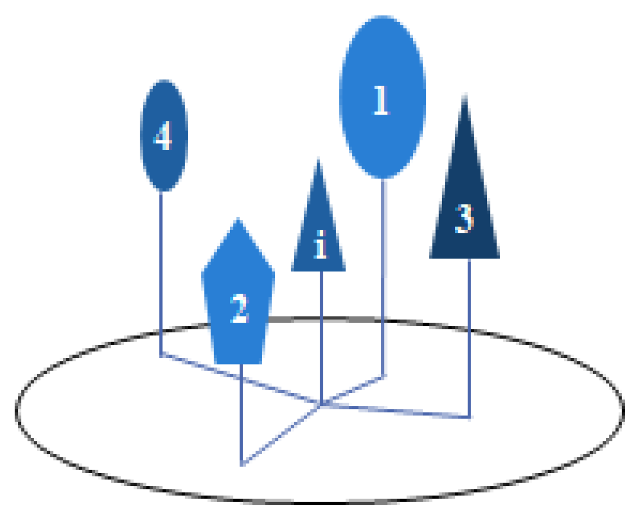
Gadow [52] and Hui et al. [44,53,54] define a structural unit as a group of n nearest neighbors to a reference tree i (Figure 1; cf. Table 1). Within the structural unit, the neighborhood-based structural indices are mingling (M_i), size dominance (U_i) and uniform angle index (W_i). These measures have proven useful for analyzing the spatial structure of forests with mixed species and sizes [38,44,45,50]. Mingling is used to express the aggregation or segregation of different species in multispecies forests and is defined as the proportion of the n nearest, heterospecific neighbors when compared with the species of reference tree i [46,52,55]. Size differentiation gives proportion of the n nearest neighbors that have a smaller size (in terms of, for example, dbh, height, crown width, etc.) than reference tree i [44,56]. The uniform angle index (W_i) describes the spatial pattern of tree locations in the neighborhood of reference tree i [44,55,56,57] and is defined as the proportion of the angle α which is less than the standard angle α₀ (72°). The angle α refers to the smaller of the two angles formed by the reference tree and the nearest two adjacent trees [44,53,56]. The values of the three spatial structure indices take the same discrete values, e.g., 0.0, 0.25, 0.5, 0.75 and 1.0 for $n=4$.

According to the definition of the three spatial measures, we can express them by a general formula as follows:

$${\omega }_i=\frac{1}{n}{{\displaystyle \sum }}_{j=1}^n{v}_j$$

(1)

where $v_j$ is a discrete variable with value$v_j$∈ {0, 1} and its meaning is related to the specific index and n is the number of nearest trees in the spatial structural unit. In this study, we took n as 4, because this value has been widely used in the literature [42,46,52] and is cost effective [58]. ${\omega }_i,$ generally, can take $n+1$ possible values, i.e., five values for $n$ = 4. The values and significance of the three parameters can be found in the literature of Hui et al. [50].

2.2. Diversity of the Structural Unit Types

According to the general formula of neighborhood-based indices Equation (1), information of location, species and size diversity can be quantified for any structural unit using the same quantification principle. The different combinations of the discrete index values can be regarded as different structural unit types (cf. Table 1). With $n$ = 4, there are $C_5^1\times C_5^1\times C_5^1=125$ possible combinations when only considering the different values of the three measures. In this formula, the symbol “C” represents combination, “1” represents one of the five values of a structural index, and “5” represents five values. However, the same mingling value may be applied to different structural unit types due to the different tree species involved.

Table 2. Structural unit types with the same mingling value.

Value of Mi	Possible Structural Unit Type	Possible Tree Species In Structural Unit Type	Number of Combination Types That May Occur with Uniform Angle Index and Size Dominance
0.00		1	$C_5^1\times C_5^1=25$
0.25		2	$C_5^1\times C_5^1=25$
0.50		2 or 3	$C_2^1\times C_5^1\times C_5^1=50$
0.75		2, 3 or 4	$C_3^1\times C_5^1\times C_5^1=75$
1.00		2, 3, 4 or 5	$C_4^1\times C_5^1\times C_5^1=100$

illustrates this phenomenon. The number of tree species in the structural unit is 1 and 2 when the mingling value is 0 and 0.25, respectively; when the mingling value is greater than 0.25, the number of tree species may be different despite having the same mingling value for the structural unit. For example, if the value of uniform angle index and size differentiation are both 0.5, when the value of mingling is 0.75, there may be 2 tree species, 3 tree species and 4 tree species in the structural unit, and these different species’ numbers define 3 different structural unit types. Therefore, according to the different combinations of each measure’s values and the number of tree species in each structural unit, there should be $(C_1^1+C_1^1+C_2^1+C_3^1+C_4^1)\times C_5^1\times C_5^1=275$ possible structural unit types. The notation meaning here is the same as above.

According to this concept, we regard structural units with the same combination characteristics as the same type, similar to different tree species in a woodland community. In analogy to species diversity, the diversity of structural unit types can be analyzed by applying, for example, the Shannon–Weiner index [59], a classical method of quantifying species diversity. It is related to the concept of entropy and widely used in ecology [60] because of its monotonic, non-negative and cumulative characteristics. Therefore, we adopted a method for expressing the diversity of structural unit types based on the Shannon–Weiner index [59] (Equation (2)).

$$D_U^{\prime }=-{\displaystyle \sum }_{i=1}^N{u}_i \log u_i$$

(2)

where $D_U^{\prime }$ is the diversity of structural unit types, $u_i$ is the proportion of the i-th structural unit type in all combination cases and $N$ is the number of structural unit types and its maximum number is 275. When there is only one structural unit type ($N=1$) in the forest, $D_U^{\prime }$ has a minimum value of zero. The more structural unit types and the more uniform the proportions, the greater the value of $D_U^{\prime }$. The maximum value of $D_U^{\prime }$ is 5.617 when $N=275$ and the $u_i$ is $1/275$.

2.3. Diversity of Stand Structure

As mentioned above, $D_U^{\prime }$ describes the diversity of the structural unit types and it is a very important aspect of the diversity of stand structure that reflects the diversity of location, species and size diversity of the n nearest trees to reference tree i in the structural unit. On the other hand, the total number of species in a stand and the size dominance of reference trees are also important aspects of the diversity of forest stands. The diversity of structural unit types only considers the tree species difference, number of tree species and relative tree size of the five trees in the structural units; therefore, we also need to consider tree species and size variation of the forest stand when we describe the diversity of stand structure. The species diversity of reference trees in a stand is also described by the proportion of stems and the Shannon–Weiner index. The tree size variation (diameter, tree height or crown diameter) in a stand, on the other hand, can be expressed by the coefficient of variation ($CV$), which can be calculated as follows:

$$CV=\sigma /\mu$$

(3)

where $\sigma$ is the standard deviation of individual tree sizes and $\mu$ is the mean value of the individual tree size. The larger the value of $CV$, the greater the variety of tree sizes in a stand. Both the Shannon–Weiner index applied to tree species diversity and $CV$ can be calculated based on the reference tree i and its n nearest neighbors for all structural units in a forest stand.

According to the above analysis and the cumulative characteristics of the Shannon–Weiner index [61] (Equation (4)), we proposed a method to express the diversity of a forest stand ($S_D^{\prime }$) as Equation (5).

$$H^{\prime }\left(AB\right)=H^{\prime }\left(A\right)+H^{\prime }\left(B\right)$$

(4)

In Equation (4), $H^{\prime }\left(AB\right)$ is the diversity of a community, $H^{\prime }\left(A\right)$ and $H^{\prime }\left(B\right)$ are the diversities of different classifications A and B, respectively, of the same community. In our study, $H^{\prime }\left(A\right)$ is the diversity of tree species and $H^{\prime }\left(B\right)$ is diversity of structural unit types. They are represented by $H^{\prime }$ and $D_U^{\prime }$ in Equation (5), respectively.

$$S_D^{\prime }=CV·(H^{\prime }+D_U^{\prime })=-CV·\left({\displaystyle \sum }_{j=1}^S{p}_j \log p_j+{\displaystyle \sum }_{i=1}^N{u}_i\log u_i\right)$$

(5)

where $S_D^{\prime }$ is the structural diversity index (cf. Table 1) based on the neighborhood-based measures, $S$ is the number of tree species in the stand, $p_i$ is the proportion of the j-th tree species in the stand; N is the number of structural unit types and u_i is the proportion of the i-th structural unit types in the stand. $CV$ is the coefficient of variation of tree size. The value of $S_D^{\prime }$, thus, is determined by the diversity of tree species, diversity of structural unit types and variation of individual tree sizes in the stand. If there is only one tree species in the stand, the diversity of structural unit types and variation of tree sizes reflects the stand diversity.

3. Study Data and Method of Analysis

Tree measurements from field plots in China, Germany, Poland, Myanmar and South Africa were analyzed to evaluate the feasibility and usefulness of the structural diversity index. The species and diameter at breast height (DBH) of every tree with a DBH greater than 5 cm were recorded in these plots. For more details of the sample plots, see

Table 3. Basic characteristics of the plots used in this study.

No.	Plot Location	Forest Type	Plot Size (m2)	Density (Trees/ha)	Richness	Mean DBH (cm)	Basal Area (m2/ha)	$\overline{\mathit{W}}$	$\overline{\mathit{M}}$	$\overline{\mathit{U}}$
1	Jianfengling, Hainan, China	Montane rainforest	30 × 100	820	84	29.2	54.87	0.533	0.963	0.515
2	Jiaohe, Jinlin (1), China	Pinus Koraiensis broad-leaved forest	100 × 100	797	19	22.4	31.67	0.491	0.828	0.493
3	Jiaohe, Jinlin (2), China	Pinus Koraiensis broad-leaved forest	100 × 100	1178	20	18.1	30.42	0.498	0.781	0.492
4	Xiaolongshan, Gansu (1), China	Oak broadleaved mixed natural forest	60 × 60	1342	49	14.6	22.79	0.491	0.806	0.493
5	Xiaolongshan, Gansu (2), China	Oak broadleaved mixed natural forest	70 × 70	933	33	19.5	27.85	0.492	0.806	0.509
6	Xiaolongshan, Gansu (3), China	Oak broadleaved mixed natural forest	65 × 50	1486	30	15.6	28.58	0.535	0.668	0.498
7	Jiulongshan, Beijing (1), China	Platycladus orientalis plantation	40 × 80	2331	8	10.5	20.26	0.428	0.200	0.494
8	Yiheyuanhou, Beijing (2), China	Pinus bungeana plantation	55 × 60	1588	1	17.7	39.2	0.383	0.000	0.495
9	Honghuaerji, Inner Mongolia (1), China	Mongolian scotch pine natural forest	100 × 100	940	1	21.3	33.6	0.463	0.000	0.494
10	Honghuaerji, Inner Mongolia (2), China	Mongolian scotch pine natural forest	100 × 100	1149	1	21.0	39.76	0.465	0.000	0.488
11	Lensahn, Germany	Beech-noble hardwood mixed forest	60 × 100	587	13	22.8	23.94	0.502	0.425	0.480
12	Manderscheid, Germany	Oak and beech mixed forest	80 × 80	381	2	31.0	28.69	0.469	0.440	0.475
13	Walsdorf, Germany	Beech and Norway spruce mixed	100 × 125	506	3	29.7	35.12	0.432	0.230	0.498
14	Knysna, South Africa	Subtropical evergreen natural forest	395 × 30	713	22	25.2	35.65	0.485	0.840	0.492
15	BialowiezaH, Poland	Temperate deciduous mixed forest	100 × 100	764	5	24.4	35.62	0.518	0.455	0.487
16	Sinthwat, Myanmar	Tropical mixed deciduous forest	100 × 100	374	56	54.1	84.09	0.512	0.883	0.500

Note: In the table, (1), (2) and (3) represent different sample plots in the same forest area.

and the Supplementary Materials. In addition, a variety of simulated thinning data based on field measurements were used to analyze the sensitivity of the new structural diversity index to stand structure changes.

4. Field Data

The data from China, obtained in Beijing, Inner Mongolia, Jilin, Gansu and Hainan provinces, are listed in the first eleven rows of Table 3. Two plots from the Beijing experiment are in Jiulongshan in western Beijing and Yiheyuanhou in northwestern Beijing. The Inner Mongolia experiments are in the Pinus sylvestris var. mongolica national nature reserve of Honghuerji, and they are natural pure forests. Two Jilin experiments represent the selectively logged temperate forest. The three Gansu experiments are in the Xiaolongshan forest region, which are in broad-leaved deciduous forests in the transition area from the warm temperate zone to the northern subtropical zone. The Hainan experiment is in the Jianfengling nature reserve and is a typical virgin tropical forest.

The data from other countries are listed in rows twelve to sixteen in Table 3. The research plot Lensahn is in a forest near the town of Lensahn in northern Germany [62]. The Walsdorf data are from a management demonstration site in the German state of Rhineland-Palatinate. Manderscheid is a temperate, deciduous forest located in the West German state of Rhineland-Palatinate [63]. The Białowieża forest stretches from eastern Poland across the border to western Belorussia [64]. The Knysna research plot is part of the “French Volume Curve” (FVC) experimental area in the evergreen forests of the Southern Cape Region of South Africa [65]. The Sinthwat research forest, which is situated near the Sinthwat village in the Paunglaung watershed of Myanmar, has been classified as a tropical mixed deciduous forest [66]. More details of the data from China and other countries are provided in the Supplementary Materials.

4.1. Simulated Thinning Data

Simulated thinning plots were used to describe the changes of stand structure diversity after management. The purpose of the simulated datasets was to test the sensitivity of the new structural diversity index to stand structure changes since controlled computer conditions brought about the changes. Simulated thinning methods include simulated thinning from above and below and thinning intensity was 10%, 20% and 30% of stem number, respectively. For simulated thinning from above, the trees were removed from larger DBH trees to smaller DBH trees according to the corresponding stem number intensity, while for simulated thinning from below, the trees were removed from smaller DBH stems to larger DBH trees according to the related stem number intensity. Based on the data of Jiaohe, Jinlin (2), and according to the above simulated thinning method, a total of 6 new plots (Jiaohe, Jinlin (2) after thinning;

Table 4. Basic characteristics of six different simulated thinning plots in Jiaohe, Jinlin (2), China.

Plot	Measure		Plot Size (m2)	Density (Trees/ha)	Number of Species in Core Area	Mean DBH (cm)	Basal Area (m2/ha)	$\overline{\mathit{W}}$	$\overline{\mathit{M}}$	$\overline{\mathit{U}}$
Jiaohe, Jinlin (2), China	Unmanaged		100 × 100	1178	20	18.1	30.42	0.498	0.781	0.492
	10%	Thinning from above	100 × 100	1060	18	13.3	14.70	0.499	0.752	0.503
		Thinning from below	100 × 100	1060	18	19.0	30.16	0.500	0.791	0.494
	20%	Thinning from above	100 × 100	942	18	11.1	9.10	0.496	0.725	0.505
		Thinning from below	100 × 100	942	18	20.1	29.81	0.488	0.802	0.498
	30%	Thinning from above	100 × 100	825	17	9.6	6.00	0.504	0.686	0.503
		Thinning from below	100 × 100	825	17	21.3	29.33	0.483	0.803	0.497

Note: In the table, (1), (2) and (3) represent different sample plots in the same forest area.

) were generated for the analysis.

4.2. Data Analysis

$CV$, $D_U^{\prime }$, $H^{\prime }$ and $S_D^{\prime }$ were calculated for each plot. DBH was used for size dominance. All data were calculated using our own R code written specifically to calculate stand diversity and forest spatial structure analysis. To eliminate the edge effect, a 3M buffer zone is set up if the sample plot area is less than 1 hectare; If the sample plot area is equal to or greater than 1 hectare, a 5 m buffer zone shall be set.

5. Results

5.1. Stand Characteristics and Spatial Pattern of Field Plots

The plots we analyzed in this study covered different forest types from cold temperate natural pure forest to tropical species-rich montane rainforest, including several plantations (Table 3). Tree densities in the 16 plots varied greatly from 374 trees per hectare in Sinthwat (plot 16) to 2331 in Jiulongshan (plot 7). Similarly, the basal area per hectare ranged from 20.3 m² to 84.09 m². The number of tree species in the plots decreased with increasing latitude from tropical montane rainforest (Jianfengling, plot 1) to cold temperate natural pure forest (Honghuaerji, plot 9 and plot 10), and the number of tree species ranged from 1 to 84 in the plots. Mean mingling $\overline{M}$ was highest in Jianfengling, plot 1, where the tree species richness was also the highest. $\overline{M}$ was 0 in a pure natural forest (Honghuaerji, plot 9 and plot 10) and in the Pinus bungeana plantation (Yiheyuanhou, plot 8), where only one tree species occurred. According to the test method of the mean uniform angle index $\overline{W}$ [67], three kinds of tree-dispersal patterns can be identified: uniform dispersal patterns, including Jiulongshan (plot 7), Honghuaerji (plot 9 and plot 10), Yiheyuanhou (plot 8), Manderscheid (plot 12) and Walsdorf (plot 13); a slighlyt clustered dispersal, including Jianfengling (plot 1), Xiaolongshan (plot 6), and Białowieża (plot 15) and all the other plots showing random distribution pattern.

5.2. Species Diversity, Size Differentiation and Structural Unit Types

The results in

Table 5. Measures of stand structure diversity of 16 different forest communities.

No.	Plot Location	No. of Species in Core Area	$\mathbf{Coefficient}\mathbf{of}\mathbf{Variation}\mathbf{of}\mathbf{dbh}\left(\mathit{C}\mathit{V}\right)$	Number of Structural Unit Types	$\mathbf{Structural}\mathbf{Unit}\mathbf{Diversity}\left({\mathit{D}}_{\mathit{U}}^{\prime }\right)$	${\mathit{H}}^{\prime }$	$\mathbf{Stand}\mathbf{Structure}\mathbf{Diversity}\left({\mathit{S}}_{\mathit{D}}^{\prime }\right)$
1	Jianfengling, China	69	0.724	45	3.452	3.851	5.287
2	Jiaohe (1), China	18	0.719	137	4.521	2.452	5.014
3	Jiaohe (2), China	18	0.735	167	4.645	2.353	5.144
4	Xiaolongshan (1), China	41	0.594	117	4.474	2.808	4.326
5	Xiaolongshan (2), China	29	0.717	106	4.373	2.609	5.006
6	Xiaolongshan (3), China	29	0.514	150	4.726	2.507	3.718
7	Jiulongshan (1), China	7	0.287	96	3.864	0.569	1.272
8	Yiheyuanhou (2), China	1	0.165	20	2.604	0.000	0.430
9	Honghuaerji (1), China	1	0.368	24	2.585	0.000	0.951
10	Honghuaerji (2), China	1	0.345	24	2.619	0.000	0.904
11	Lensahn, Germany	13	0.751	92	4.150	1.222	4.034
12	Manderscheid, Germany	2	0.439	60	3.799	0.623	1.941
13	Walsdorf, Germany	3	0.376	83	3.909	0.730	1.744
14	Knysna, South Africa	21	0.512	128	4.477	2.517	3.581
15	BialowiezaH, Poland	5	0.866	138	4.535	1.020	4.811
16	Sinthwat, Myanmar	56	0.637	89	4.110	3.331	4.740

Note: In the table, (1), (2) and (3) represent different sample plots in the same forest area.

show the characteristics of the plot core area. The highest $H^{\prime }$ was in the mountain rainforest in Hainan, China, followed by the tropical mixed deciduous forest of Sinthwat, Myanmar. $H^{\prime }$ was zero for the Pinus sylvestris var. mongolica natural forest (plot 9 and plot 10) and Pinus bungeana plantation (plot 8) because there was only one species in those plots. The coefficient of variation of DBH ($CV$) of different forest plots varied greatly. The largest $CV$ was in Białowieża, plot 15, followed by that of Lensahn, plot 11. The smallest$CV$ of 0.165 was calculated in the Pinus bungeana plantation in Beijing (plot 8). In terms of the number of structural unit types in the plots, the numbers were between 20 in Yiheyuanhou, plot 8, and 167 in Jiaohe (2), plot 3. There is a trend that the structural unit types of mixed-species forests were higher than those of pure forests. The diversity of structural units in Table 5 shows that the value of $D_U^{\prime }$ ranged from 2.585 in Honghuaerji, China (plot 9), to 4.726 in Xiaolongshan (3), China (plot 6). The corresponding numbers of structural unit types were 24 and 150, respectively. The highest and lowest numbers of structural unit types in the 16 plots in Jiaohe (2), China (plot 3) and in Yiheyuanhou, China (plot 8), and the corresponding values of $D_U^{\prime }$, were 4.645 and 2.604, respectively. These results show that the diversity of structural unit types is related to the richness of structural unit types and the uniformity of distribution of structural unit types.

5.3. Stand Structural Diversity Index ($S_D^{\prime }$)

In terms of the structural diversity index $S_D^{\prime }$ (Table 5), the mountain rainforest in Hainan (plot 1) had the highest value, followed by the broad-leaved Korean pine forest in Jiaohe (2), plot 3, broad-leaved Korean pine forest in Jiaohe (1), plot 2, and oak broadleaved mixed natural forest in Xiaolongshan (2), plot 5 (cf. table. 5). Among all plots, the $S_D^{\prime }$ values of plantations and pure natural forests were lower, and the lowest was 0.430 and found in the Pinus bungeana plantation (plot 8). Interestingly, the number and diversity of the structural unit types of the Hainan Mountain rainforest (plot 1) were relatively lower than other plots. The main reason for this was that the structural unit types were dominated by mingling values of one, however, this stand had the highest diversity of stand structures because it had the highest tree species diversity. Another interesting result is the stand structure diversity of Białowieża, Poland (plot 15). In this stand, there were only five tree species, and the value of $H^{\prime }$ was only 1.020; however, the corresponding DBH coefficient of variation and the diversity of structural unit types was relatively high, which led to a stand structural diversity ($S_D^{\prime }$) higher than those of Sinthwat, Myanmar (plot 16), Knysna, South Africa (plot 14), Lensahn, Germany (plot 11), Xiaolongshan (1) and Xiaolongshan (3) (plot 4 and plot 6) and Jiulongshan (1) (plot 7), China, despite the higher number and diversity of tree species in these plots. In addition, two pure natural forests of Pinus sylvestris var. mongolica had the same tree species number and structural unit types, but they had different stand structure diversity due to different $CV$ and $D_U^{\prime }$.

5.4. Effects of Management Activities on Stand Structure Diversity Index

Some changes have taken place in the stand structure diversity ($S_D^{\prime }$) of the simulated thinning with different intensities and in different forest canopy layers of the Pinus koraiensis broad-leaved forest in Jiaohe, Jilin (2), China (Table 4 and

Table 6. Comparison of stand structure diversity of six different simulated thinning methods in Jiaohe, Jinlin (2), China.

Plot	Measure		$\mathit{C}\mathit{V}$	No. of Structural Unit Type	$\mathbf{Structural}\mathbf{Unit}\mathbf{Diversity}\left({\mathit{D}}_{\mathit{U}}^{\prime }\right)$	${\mathit{H}}^{\prime }$	$\mathbf{Stand}\mathbf{Structure}\mathbf{Diversity}\left({\mathit{S}}_{\mathit{D}}^{\prime }\right)$
Jiaohe, Jinlin (2), China	Unmanaged		0.735	167	4.645	2.353	5.144
	10%	Thinning from above	0.509	181	4.776	2.254	3.578
		Thinning from below	0.692	156	4.625	2.393	4.856
	20%	Thinning from above	0.418	179	4.772	2.155	2.895
		Thinning from below	0.644	155	4.586	2.422	4.513
	30%	Thinning from above	0.345	173	4.768	2.030	2.346
		Thinning from below	0.605	143	4.494	2.443	4.196

Note: In the table, (1), (2) and (3) represent different sample plots in the same forest area.

). The results show that the thinning had almost no effect on the overall tree dispersal pattern but significantly impacted mingling, size dominance and the number of tree species of the forest. After the thinning, the number of tree species was reduced from 20 to 17, while the mean mingling and $H^{\prime }$ increased as a result of thinning from below. The size differentiation clearly decreased, as can be seen from the reduction in the coefficient of variation after the interventions, especially after the thinning from above. The thinning from above increases the number of structural unit types, while the thinning from below tends to have the opposite effect. The change in the diversity of the structural unit type ($D_U^{\prime }$) is consistent with the number of structural unit types. The values of stand structural diversity ($S_D^{\prime }$) of different thinning methods and intensities have decreased after thinning compared with the unmanaged treatment, and the greater the thinning intensity, the greater the change range. The value of $S_D^{\prime }$ was 5.144 before thinning. After thinning from above with a stem-number removal of 10%, 20% and 30%, the values were 3.578, 2.895 and 2.346, respectively. In addition, the value of $S_D^{\prime }$ decreased after the thinning from above more than after the thinning from below when applied the same thinning intensity. For example, the value of $S_D^{\prime }$ decreased from 5.144 to 3.578 and 4.856 after thinning from above and below, respectively, at the same thinning intensity. These results suggest that the structural diversity index $S_D^{\prime }$ can well reflect the changes in stand structure. What needs to be explained here is that we did not evaluate the advantages and disadvantages of the thinning methods but emphasized the sensitivity of the new stand structure diversity index to management activities.

6. Discussion

A measure of stand structural diversity is intuitively appealing if it can be used to compare the diversity across different ecosystems, not only in terms of the mere number of tree species but also by considering size differences and individual tree distribution. In this study, by combining tree species diversity, size differences and structure unit type diversity and by using the Shannon–Weiner diversity model, we can fully describe the diversity of stand structure in a comprehensive approach. The test results of 16 forest stands indicated that the information contained in the new structural diversity ($S_D^{\prime }$) far exceeds the tree species diversity index that the diversity increases with the increase in the number of tree species. For example, when comparing the two plots in Jiaohe (plot 2 and plot 3) and the plot in Białowieża (plot 15), which are all located in the cold temperate zone, with the plots Gansu (plot 4, plot 5 and plot 6) and Myanmar (plot 16), which are located in the transition from the temperate zone to subtropical and tropical zones. While Jiaohe and Białowieża only include 18 and 5 tree species, respectively, their structural diversity index values are higher than those in Gansu and Myanmar with 30 to 56 tree species. This is mainly due to the higher number and diversity of structural unit types and the size differentiation of individual trees in the plots. Another reason for the high structural diversity value in Białowieża (plot 15) is that the stand was managed according to the principles of continuous cover forestry [64], which increased the diversity of structural unit types and the coefficient of variation of DBH even beyond natural diversity levels. In addition, the new stand structure diversity index can not only calculate the structural diversity of mixed species forests but can also be used to calculate the structural diversity of pure forests. There is only one tree species in the pure forest, and the contribution of tree species to the diversity of stand structure is zero. The difference in structure between pure forests was mainly due to the size differentiation and the dispersal of individual trees, as the traditional biodiversity index is non-spatial and cannot reflect this variation. This is a clear advantage of the new structural diversity index. Of course, we can also use other characteristic attributes of stand to distinguish the structural diversity of pure forests, such as the composition diversity of basal area, standard deviation of diameter at breast height and total tree height, foliage height diversity and so on. The results for three pure forests (Yiheyuanhou (2), Honghuaerji (1) and Honghuaerji (2)) indicate that the structural diversity of natural monocultural forests is higher than that of artificially planted pure forests because the individuals have a greater spatial size diversity and a more irregular dispersal.

Thinning from above or below are traditional forest management methods, which are used to selectively cut trees in order to improve stand growth rate [68] and obtain a certain amount of wood [69] and non-wood forest products [70]. There is rarely a focus on structural diversity. Different management methods profoundly impact the diversity of forest structure by decreasing or increasing individual tree size differentiation by changing the dispersal pattern of trees or by reducing the number of tree species. Evaluating the management activities to improve the diversity of stand structure is particularly important. The results of the simulated thinning with different intensities and thinning types show that the structural diversity index can well reflect management events. Different management methods produce different results, and the greater the intensity of artificial management or disturbance, the greater is the change in the structural diversity index accounting for changes in forest structure diversity. Employing forest management to speed up the development of a forest stand towards a more diverse ecosystem has become an international trend [71]. Tree size diversity, dispersal pattern and species composition are the primary structural properties considered in forest management [72,73]. In recent years, some management methods have paid attention to improving the diversity of forest structure. Near-natural forest management (NNFM) [9,10] was developed and improved on the basis of the classic idea of continuous cover forest (CCF). It believes that forest silviculture and management should be as close to the “potential natural vegetation” as possible. The closer the stand structure is to nature, the more stable the forest is, and the healthier and safer the forest is. There are many successful examples in Germany. Structure-based forest management (SBFM), which was put forward by Hui et al., also originated from CCF, but it pays more attention to creating and maintaining the best stand structure [11]. The core technology of SBFM is to apply spatial structure parameters to guide stand spatial structure optimization. The extensive management practice has been carried out and have achieved good management results in different forest types of mixed forests in China [48]. Therefore, the feature of simultaneously expressing diversity of tree species, size and distribution can well reflect management activities of increasing stand structural diversity is important and it can be applied to guide specific forest management to improve stand structure diversity.

In the analysis, tree DBH was used as a comparative indicator of tree size differentiation because DBH data are easy to obtain and accurate. However, crown size or tree height can also be used as comparative indicators of size differentiation. The value of $S_D^{\prime }$ can be assessed as part of a routine forest survey at almost no additional cost. After selecting the reference tree, its n nearest neighbors and their species needs to be identified in terms of a structural unit, possibly in the field. If tree coordinates are not measured, we can also use the routine forest survey to collect the diversity data and additional measurements are not needed.

7. Conclusions

According to our analysis, the new structural diversity index ($S_D^{\prime }$) at stand scale has at least four characteristics of other diversity indexes. Firstly, it provides minimum and maximum values for different structural unit types in forests to achieve a unified comparative basis for calculating forest structure diversity. Secondly, the new method takes three factors simultaneously into account when calculating forest structure diversity, i.e., the tree dispel pattern, size differences and tree species. Researchers and managers can choose different indicators of size differentiation according to their focus. Thirdly, the new index can well reflect the stand structure changes to evaluate the impact of management activities on the diversity of stand structure. Thus, the index can be applied to guide the improvement of stand structure. Last but not least, the new structural diversity index can not only calculate the structural diversity of mixed species forests but can also be used to calculate the structural diversity of pure forests.

References

- Pretzsch, H.; Zenner, E.K. Toward managing mixed-species stands: From parametrization to prescription. For. Ecosyst. 2017, 4, 19. [Google Scholar] [CrossRef] [Green Version]
- Lei, X.; Tang, S. Indicators of structural diversity within stand: Review. Sci. Silvae Sin. 2002, 38, 141–146. [Google Scholar]
- Lähde, E.; Laiho, O.; Norokorpi, Y. Diversity-oriented silviculture in the boreal zone of Europe. For. Ecol. Manag. 1999, 118, 223–243. [Google Scholar] [CrossRef]
- Buongiorno, J.; Dahir, S.; Lu, H.; Lin, C. Tree size diversity and economic returns in uneven-aged forest stands. For. Sci. 1994, 40, 83–103. [Google Scholar]
- O’Hara, K.L. Silviculture for structural diversity: A new look at multi aged systems. J. For. 1998, 96, 4–10. [Google Scholar] [CrossRef]
- Franklin, J.F.; Spies, T.A.; Van Pelt, R.; Carey, A.B.; Thornburgh, D.A.; Berg, D.R.; Lindenmayer, D.B.; Harmon, M.E.; Keeton, W.S.; Shaw, D.C.; et al. Disturbances and structural development of natural forest ecosystems with silvicultural implications, using Douglas-Fir forests as an example. For. Ecol. Manag. 2002, 155, 399–423. [Google Scholar] [CrossRef]
- Lei, X.; Wang, W.; Peng, C. Relationships between stand growth and structural diversity in spruce-dominated forests in New Brunswick. Can. J. For. Res. 2009, 39, 1835–1847. [Google Scholar] [CrossRef]
- Valbuena, R.; Packalén, P.; Martı, S.; Fernández, N.; Maltamo, M. Diversity and equitability ordering profiles applied to study forest structure. For. Ecol. Manag. 2012, 276, 185–195. [Google Scholar] [CrossRef] [Green Version]
- O’Hara, K.L. The silviculture of transformation—A commentary. For. Ecol. Manag. 2001, 151, 81–86. [Google Scholar] [CrossRef]
- O’Hara, K.L. Multiaged Silviculture Oxford: Managing for Complex Forest Stand Structure; Oxford University Press: Oxford, UK, 2014; 213p. [Google Scholar]
- Hui, G.; Gadow, K.V.; Hu, Y.B.; Xu, H. Structure-Based Forest Management; China Forestry Press: Beijing, China, 2007; pp. 29–36. [Google Scholar]
- Staudhammer, C.L.; Lemay, V.M. Introduction and evaluation of possible indices of stand structural diversity. Can. J. For. Res. 2001, 31, 1105–1115. [Google Scholar] [CrossRef]
- MacArthur, R.H.; MacArthur, J.W. On bird species diversity. Ecology 1961, 42, 594–598. [Google Scholar] [CrossRef]
- Holland, D.N.; Lilieholm, R.J.; Roberts, D.W.; Gilless, J.K. Economic trade-offs of managing forests for timber production and vegetative diversity. Can. J. For. Res. 1994, 24, 1260–1265. [Google Scholar] [CrossRef]
- Volin, L.; Buomgiorno, J. Effect of alternative management regimes on forest stand structure, species composition and income: A model for the Italian Dolomites. For. Ecol. Manag. 1996, 87, 107–125. [Google Scholar] [CrossRef]
- Spies, T.A.; Franklin, J.F. The structure of natural young, mature, and old-growth Douglas-Fir forests in Oregon and Washington. In Wildlife and Vegetation of Unmanaged Douglas-Fir Forests; Aubry, K.B., Brookes, M.H., Agee, J.K., Anthony, R.G., Franklin, J.F., Eds.; USDA Forest Service: Portland, OR, USA, 1991; pp. 91–109. [Google Scholar]
- Zenner, E.K. Do residual trees increase structural complexity in Pacific Northwest coniferous forests? Ecol. Appl. 2000, 10, 800–810. [Google Scholar] [CrossRef]
- Neumann, M.; Starlinger, F. The significance of different indices for stand structure and diversity in forests. For. Ecol. Manag. 2001, 145, 91–106. [Google Scholar] [CrossRef]
- Svensson, J.S.; Jeglum, J.K. Structure and dynamics of an undisturbed old-growth Norway spruce forest on the rising Bothnian coastline. For. Ecol. Manag. 2001, 151, 67–79. [Google Scholar] [CrossRef]
- Dewalt, S.J.; Maliakal, S.K.; Denslow, J.S. Changes in vegetation structure and composition along a tropical forest chrono sequence: Implications for wildlife. For. Ecol. Manag. 2003, 182, 139–151. [Google Scholar] [CrossRef]
- Bachofen, H.; Zingg, A. Effectiveness of structure improvement thinning on stand structure in subalpine Norway spruce (Picea abies (L.) Karst.) stands. For. Ecol. Manag. 2001, 145, 137–149. [Google Scholar] [CrossRef]
- Sullivan, T.P.; Sullivan, D.S.; Lindgren, P.M.F. Stand structure and small mammals in young Lodgepole Pine forest: 10-year results after thinning. Ecol. Soc. Am. 2001, 11, 1151–1173. [Google Scholar] [CrossRef]
- Gove, J.H.; Patil, G.P.; Taillie, C. A mathematical programming model for maintaining structural diversity in uneven-aged forest stands with implications to other formulations. Ecol. Model. 1995, 79, 11–19. [Google Scholar] [CrossRef]
- Barnett, J.L.; How, R.A.; Humphreys, W.F. The use of habitat components by small mammals in eastern Australia. Aust. J. Ecol. 1978, 3, 277–285. [Google Scholar] [CrossRef]
- Newsome, A.E.; Catling, P.C. Habitat preferences of mammals inhabiting heathlands of warm temperate coastal, montane and alpine regions of southeastern Australia. In Ecosystems of the World 9A. Heathlands and Related Shrublands. Descriptive Studies; Specht, R.L., Ed.; Elsevier: Amsterdam, The Netherlands, 1979; pp. 301–316. [Google Scholar]
- Van Den Meersschaut, D.; Vandekerkhove, K. Development of a stand-scale forest biodiversity index based on the State Forest Inventory. In Integrated Tools for Natural Resources Inventories in the 21st Century; Hansen, M., Burk, T., Eds.; USDA: Boise, ID, USA, 1998; pp. 340–349. [Google Scholar]
- Roy, A.; Tripathi, S.K.; Basu, S.K. Formulating diversity vector for ecosystem comparison. Ecol. Model. 2004, 179, 499–513. [Google Scholar] [CrossRef]
- Holdridge, L.R. Life Zone Ecology; Tropical Science Center: San Jose, CA, USA, 1967. [Google Scholar]
- Jaehne, S.; Dohrenbusch, A. Ein Verfahren zur Beurteilung der Bestandesdiversität. Summary: A method to evaluate forest stand diversity. Forstwiss. Cent. 1996, 116, 333–345. [Google Scholar] [CrossRef]
- Gavrikov, V.; Stoyan, D. The use of marked point processes in ecological and environmental forest studies. Environ. Ecol. Stat. 1995, 2, 331–344. [Google Scholar] [CrossRef]
- Pommerening, A.; Rodriguez-Soalleiro, R. Species mingling and diameter Differentiation as second-order characteristics. Allg. Forst Jagdztg. 2011, 182, 115–129. [Google Scholar]
- Wiegand, T.; Moloney, K.A. Handbook of Spatial Point-Pattern Analysis in Ecology; CRC Press: Boca Raton, FL, USA, 2013; p. 538. [Google Scholar]
- Hui, G.; Pommerening, A. Analysing tree species and size diversity patterns in multi-species uneven-aged forests of Northern China. For. Ecol. Manag. 2014, 316, 125–138. [Google Scholar] [CrossRef]
- Pommerening, A.; Särkkä, A. What mark variograms tell about spatial plant interactions. Ecol. Mod. 2013, 251, 64–72. [Google Scholar] [CrossRef]
- Pommerening, A.; Grabarnik, P. Individual-Based Methods in Forest Ecology and Management; Spring Nature Switzerland AG: Cham, Switzerlamd, 2019; pp. 110–197. [Google Scholar]
- Gadow, K.V. Waldstruktur und Diversität [Forest structure and diversity]. Allg. Forst J.-Zeitung 1999, 170, 117–122. [Google Scholar]
- Pommerening, A. Approaches to quantifying forest structures. Forestry 2002, 75, 305–324. [Google Scholar] [CrossRef]
- Pommerening, A. Evaluating structural indices by reversing forest structural analysis. For. Ecol. Manag. 2006, 224, 266–277. [Google Scholar] [CrossRef]
- Ferris, R.; Humphrey, J.W. A review of potential biodiversity indicators for application in British forests. Forestry 1999, 72, 313–328. [Google Scholar] [CrossRef]
- Noss, R.F. Indicators for monitoring biodiversity: A hierarchical approach. Conserv. Biol. 1990, 4, 355–364. [Google Scholar] [CrossRef]
- Prodan, M. Punkstichprobe fuÈr die Forsteinrichtung. Forst Holzwirt. 1968, 23, 225–226. (In German) [Google Scholar]
- Albert, M.; Gadow, K.V. Assessing biodiversity with new neighborhood-based parameters. In Data Management and Modelling Using Remote Sensing and GIS for Tropical Forest Land Inventory; Rodeo International Publishers, 1999; pp. 433–445. Available online: https://www.researchgate.net/publication/304283982_Assessing_Biodiversity_with_New_Neighborhood-Based_Parameters (accessed on 4 January 2022).
- Kint, V.; Meirvenne, M.V.; Nachtergale, L.; Geudens, G.; Lust, N. Spatial methods for quantifying forest stand structure development: A comparison between nearest-neighbor indices and variogram analysis. For. sci. 2003, 49, 36–49. [Google Scholar]
- Hui, G.; Albert, M.; Gadow, K.V. Das Umgebungsmab als parameter zur Nachbildung von bestandesstrukturen. Forstwiss. Cent. 1998, 117, 258–266. [Google Scholar] [CrossRef]
- Graz, F.P. The behaviour of the species mingling index Msp in relation to species differentiation and dispersion. Eur. J. For. Res. 2004, 123, 87–92. [Google Scholar] [CrossRef]
- Hui, G.; Zhao, X.; Zhao, Z.; Gadow, K.V. Evaluating tree species spatial diversity based on neighborhood relationships. For. Sci. 2011, 57, 292–300. [Google Scholar] [CrossRef]
- Li, Y.; Hui, G.; Zhao, Z.; Hu, Y. The bivariate distribution characteristics of spatial structure in natural Korean pine broad-leaved forest. J. Veg. Sci. 2012, 23, 1180–1190. [Google Scholar] [CrossRef]
- Li, Y.; Hui, G.; Zhao, Z.; Hu, Y.; Ye, S. Spatial structural characteristics of three hardwood species in Korean pine broad-leaved forest-Validating the bivariate distribution of structural parameters from the point of tree population. For. Ecol. Manag. 2014, 314, 17–25. [Google Scholar] [CrossRef]
- Zhao, Z.; Liu, W.; Shi, X.; Li, A.; Hui, G. Structure Dynamic of Quercus aliena var. acuteserrata Natural Forest on Xiaolongshan. For. Res. 2015, 28, 759–766. [Google Scholar]
- Hui, G.; Zhang, G.; Zhao, Z.; Yang, A. Methods of Forest Structure Research: A Review. Curr. For. Rep. 2019, 5, 142–154. [Google Scholar] [CrossRef]
- Zhang, G.; Hui, G.; Zhang, G.; Zhao, Z.; Hu, Y. Telescope method for characterizing the spatial structure of a pine–oak mixed forest in the Xiaolong Mountains, China. Scand. J. For. Res. 2019, 34, 751–762. [Google Scholar] [CrossRef]
- Gadow, K.V. Zur Bestandesbeschreibung in der Forsteinrichtung. [New variables for describing stands of trees]. Forst Holzwirt. 1993, 48, 602–606. [Google Scholar]
- Hui, G.; Gadow, K.V. Das Winkelmass-Theoretische Überlegungen zum optimalen Standardwinkel. Allg. Forst J.-Zeitung 2002, 173, 1–10. [Google Scholar]
- Hui, G.; Albert, M. Stichprobensimulationen zur Schätzung nachbarschaftsbezogener Strukturparameter in Waldbeständen (Simulation studies for estimating neighborhood-based structural parameters in forest stands). Allg. Forst J.-Zeitung 2004, 175, 199–209. [Google Scholar]
- Füldner, K. Strukturbeschreibung von Buchen-Edellaubholz-Mischwäldern. (Describing Forest Structures in Mixed Beech-Ash-Maple-Sycamore Stands). Ph.D. Thesis, Faculty of Forestry, University of Göttingen, Cuvillier Verlag Göttingen, Göttingen, Germany, 1995; 163p. [Google Scholar]
- Aguirre, O.; Hui, G.; Gadow, K.V.; Jimenez, J. An analysis of spatial forest structure using neighbourhood-based variables. For. Ecol. Manag. 2003, 183, 137–145. [Google Scholar] [CrossRef]
- Gadow, K.V.; Hui, G.; Albert, M. Das Winkelmab-ein Strukturparameter zur Beschreibung der Individualverteilung inWaldbeständen. Cent. Gesamte Forstwes. 1998, 115, 1–10. [Google Scholar]
- Wang, H.; Zhang, G.; Hui, G.; Li, Y.; Hu, Y.; Zhao, Z. The influence of sampling unit size and spatial arrangement patterns on neighborhood-based spatial structure analyses of forest stands. For. Syst. 2016, 25, e056. [Google Scholar] [CrossRef] [Green Version]
- Shannon, C.E.; Weaver, W. The Mathematical Theory of Communication; University of Illinois Press: Urbana, IL, USA, 1949; 117p. [Google Scholar]
- Magurran, A.E. Measuring of Biological Diversity. Environ. Ecol. Stat. 2004, 1, 95–103. [Google Scholar] [CrossRef]
- Khinchin, A.I. Mathematical foundations of information theory. Am. Math. Mon. 1957, 66, 159–160. [Google Scholar]
- Gadow, K.V.; Tremer, N.; Mylius, A. Datengewinnung für die Forsteinrichtungsforschung. Forst Holz 2005, 61, 60–65. [Google Scholar]
- Uria-Diez, J.; Pommerening, A. Crown plasticity in Scots pine (Pinus sylvestris L.) as a strategy of adaptation to competition and environmental factors. Ecol. Mod. 2017, 356, 117–126. [Google Scholar] [CrossRef]
- Pommerening, A.; Murphy, S.T. A review of the history, definitions and methods of continuous cover forestry with special attention to afforestation and restocking. Forestry 2004, 77, 27–44. [Google Scholar] [CrossRef] [Green Version]
- Kempka, C.; Gadow, K.V. Eine Strukturanalyse im Naturwald von Knysna. Forstarchiv 1998, 69, 235–239. [Google Scholar]
- Zin, M.T. Developing a Scientific Basis for Sustainable Management of Tropical Forest Watersheds: Case Studies from Myanmar; Universitätsverlag Göttingen: Göttingen, Germany, 2005. [Google Scholar] [CrossRef] [Green Version]
- Zhao, Z.; Hui, G.; Hu, Y.; Wang, H.; Zhang, G.; Gadow, K.V. Testing the significance of different tree spatial distribution patterns based on the uniform angle index. Can. J. For. Res. 2014, 44, 1419–1425. [Google Scholar] [CrossRef]
- Cassidy, M.; Palmer, G.; Glencross, K.; Nichols, J.D.; Smith, R.G.B. Intensity of thinning affects log size and value in Eucalyptus pilularis. For. Ecol. Manag. 2012, 264, 220–227. [Google Scholar] [CrossRef]
- Mäkinen, H.; Isomäki, A. Thinning intensity and long-term changes in increment and stem form of Scots pine trees. For. Ecol. Manag. 2004, 203, 21–34. [Google Scholar] [CrossRef]
- Bonet, J.A.; de-Miguel, S.; de Aragon, J.M.; Pukkala, T.; Palahi, M. Immediate effect of thinning on the yield of Lactarius group deliciosus in Pinuspinaster forests in northeastern Spain. For. Ecol. Manag. 2012, 265, 211–217. [Google Scholar] [CrossRef]
- Kuuluvainen, T. Natural variability of forests as a reference for restoring and managing biological diversity in boreal Fennoscandia. Silva Fenn. 2002, 36, 97–125. [Google Scholar] [CrossRef] [Green Version]
- Kint, V. Structural development in ageing temperate Scots pine stands. For. Ecol. Manage 2005, 214, 237–250. [Google Scholar] [CrossRef]
- Kint, V.; Lust, N.; Ferris, R.; Olsthoorn, A.F.M. Quantification of forest stand structure applied to Scots pine (Pinus sylvestris L.) forests. Investig. Agrar. Sist. Recur. For. Fuera Serie 2000, 1, 147–163. [Google Scholar]
Figure 1.
Stand spatial structural unit. i is the reference tree, and 1, 2, 3 and 4 are the four nearest neighbor trees.