Research on the Temporal and Spatial Distributions of Standing Wood Carbon Storage Based on Remote Sensing Images and Local Models

Abstract

Background and Objectives: It is important to understand the temporal and spatial distributions of standing wood carbon storage in forests to maintain ecological balance and forest dynamics. Such information can provide technical and data support for promoting ecological construction, formulating different afforestation policies, and implementing forest management strategies. Long-term series of Landsat 5 (Thematic Mapper, TM) and Landsat 8 (Operational Land Imager, OLI) remote sensing images and digital elevation models (DEM), as well as multiphase survey data, provide new opportunities for research on the temporal and spatial distributions of standing wood carbon storage in forests. Methods: The extracted remote sensing factors, terrain factors, and forest stand factors were analyzed with stepwise regression in relation to standing wood carbon storage to identify significant influential factors, build a global ordinary least squares (OLS) model and a linear mixed model (LMM), and construct a local geographically weighted regression (GWR), multiscale geographically weighted regression model (MGWR), temporally weighted regression (TWR), and geographically and temporally weighted regression (GTWR). Model evaluation indicators were used to calculate residual Moran’s I values, and the optimal model was selected to explore the spatiotemporal dynamics of standing wood carbon storage in the Liangshui Nature Reserve. Results: Remote sensing factors, topographic factors (Slope), and stand factors (Age and DBH) were significantly correlated with standing wood carbon storage, and the constructed global models exhibited fitting effects inferior to those of the established local models. LMM is also used as a global model to add random effects on the basis of OLS, and R² is increased to 0.52 compared with OLS. The local models based on geographically weighted regression, namely, GWR, MGWR, TWR, and GTWR, all have good performance. Compared with OLS, the R² is increased to 0.572, 0.589, 0.643, and 0.734, and the fitting effect of GTWR is the best. GTWR can overcome spatial autocorrelation and temporal autocorrelation problems, with a higher R² (0.734) and a more ideal model residual than other models. This study develops a model for carbon storage (CS) considering various influential factors in the Liangshui area and provides a possible solution for the estimation of long-term carbon storage distribution.

1. Introduction

Forests, as one of the most important components of the Earth’s biosphere, are plant communities dominated by trees and composed of a variety of plants, animals, and microorganisms. Forest carbon storage is the amount of carbon stored in a forest and is related to the quality of forest carbon and the total amount of material. As the largest carbon pool in terrestrial ecosystems, forest ecosystems are both carbon sinks and carbon sources. The carbon cycle process plays a vital role in climate change, atmospheric circulation, and biodiversity [1]. In addition, the estimation of carbon storage is helpful for evaluating the bioenergy of some landscapes, promoting the coordinated development of ecological components and monitoring the sustainability of forest resources [2]. Additionally, climate change is an important issue facing humankind. To actively respond to climate change, green and low-carbon development paths are being established, and sustainable development is being promoted; notably, China has proposed measures to achieve carbon neutrality by 2060 [3]. Studies of forest carbon storage can help achieve this goal and aid countries around the world in coping with climate change. Therefore, research on the dynamic temporal and spatial distributions of standing wood carbon storage can provide technical and data support for promoting ecological construction, formulating different afforestation policies, and effectively implementing forest management strategies [4].

The carbon storage of standing wood in forests is calculated based on field survey data. The ground survey method is highly credible, but it is cumbersome and can cause certain damage to the forest. Moreover, traditional surveys are not ideal for dynamically monitoring forest carbon storage over a large area [5]. In particular, large-scale surveys of natural forests in the Liangshui Nature Reserve are bound to cause damage to the local ecology. Remote sensing and sample data have been combined for the explicit estimation of carbon storage in forests [6]. Diverse types of remote sensing data, such as optical sensor data, light detection and ranging data (lidar) and radio detection and ranging data (radar), each of which has different advantages and disadvantages, can be used in carbon storage estimates [7,8]. With continuous improvements to remote sensing data in terms of temporal, spatial, and spectral resolutions, such data can be used in carbon balance assessments in terrestrial and forest ecosystems. Using remote sensing to monitor forest dynamics has developed from single-band estimation to vegetation index estimation to microwave technology, and many scientific researchers have made efforts [9]. K. Narmada [10] used the NDVI (standardized difference vegetation index) to estimate the amount of carbon sequestered in the mangroves that grew in the Mutupet region from 2000 to 2017. Experiments have verified the reliability of high-resolution aerial remote sensing data and yielded good results. Near-red spectroscopy experiments were also performed in this study to estimate the mangrove carbon reserves grown in this area. Inspired by this study, other remote sensing factors, including NDVI, such as the ratio acquisition index (RVI) and difference acquisition index (DVI), were selected for research to determine if they can be applied to the study of forest standing wood carbon storage, and it was found that they also have good results. Then, the red and near red spectra were further studied. It was found that the texture characteristics of the two spectra were also related to the standing wood carbon storage.

In this study, regression models were used to estimate the carbon storage in standing trees in forests. The most common model is the traditional global model fitted by the ordinary least squares (OLS) model [11]. The linear mixed model (LMM) is an extension of the ordinary least squares model. The OLS approach is applicable to entire regions, and it is a fixed-effect model based on the dependent variable. In contrast, the LMM considers random effects, so the fitting estimation is better than that of the least squares approach [12]. Both the OLS and LMM methods are established based on the basic assumption that the distribution of carbon stocks is random, without taking into account the spatial nonstationarity of the research variables. Lianjun Zhang [13] used OLS, LMM, generalized additive model (GAM), and GWR to study the correlation between stand variables, pointed out that there is a very important relationship between tree growth and environmental impact, and studied the changes in competition among trees. This study has verified that spatial correlations among samples are often associated with geographic proximity. GWR skillfully considers the spatial characteristics of the data in regression analysis [14], and tests have shown that the GWR estimation effect is better than that of the OLS model. On the basis of GWR, a multiscale geographically weighted regression model (MGWR) is proposed; this model relaxes the assumption that all the processes to be modeled are of the same spatial scale, as assumed in GWR, and the fitting effect is better than that of GWR [15].

Although GWR estimations are considerably better than those of OLS, there are still certain shortcomings of GWR methods. GWR models can only model cross-sectional data [16] without considering the temporal influence. Geographically and temporally weighted regression (GTWR) is performed in time and space in this study to predict and analyze forest carbon storage in the Liangshui Reserve. GTWR can simultaneously consider spatial and temporal nonstationarity. At present, the GTWR model is widely used in ecology and economics, and the first application of GTWR was by A. Stewart Fotheringham [17]. To consider local impacts in space and time, GTWR was developed and used to analyze the changes in housing prices in London from 1980 to 1998. The fitting effect was found to be better than that of GWR, highlighting the importance of time and latitude in modeling [18]. Hone-Jay Chu [19] used GTWR and random sample consistency (RANSAC) models to solve the AOD-PM_2.5 estimation problem through effective sampling and fitting, and the proposed method effectively produced the relationship between the observed PM_2.5 and AOD data. It is also proved that GTWR has certain advantages in overcoming the influence of spatiotemporal heterogeneity. Wei [16] used GTWR to investigate the relationship between PM_2.5 and standard air pollutants (SO₂, NO₂, PM₁₀, CO, and O₃) in Heilongjiang Province, China, from 2015 to 2018, and compared the model with other basic models; they found that temporal and spatial heterogeneity influenced the distribution of data, and the GTWR fitting effect was better than that of other basic models such as OLS. Inspired by such work, we will investigate whether the distribution of forest standing tree carbon stocks is affected by spatial and temporal heterogeneity, and that the distribution of forest standing trees carbon storage also has a high degree of spatial and temporal heterogeneity, which has a great impact on the fitting and prediction of the model. How to overcome this impact has become the focus of research.

In this study, we evaluated the fitting effect of different models on forest standing tree carbon storage. Specific objectives include (1) screening the predictors significantly related to the carbon storage of standing trees; (2) determining the relationship between forest standing tree carbon stocks and predictors; (3) comparing the fitting effect of the global model (OLS and LMM) and the local model (GWR, MGWR, TWR and GTWR), and conducting spatial autocorrelation analysis; (4) the space analysis and error analysis of the optimal model are carried out. The innovation of this paper is that the time and space factors are introduced into the model fitting, which further improves the fitting effect. The purpose of this study is to use readily available stand data and remote sensing data to predict standing wood carbon storage and improve the efficiency of forest management.

2. Materials and Methods

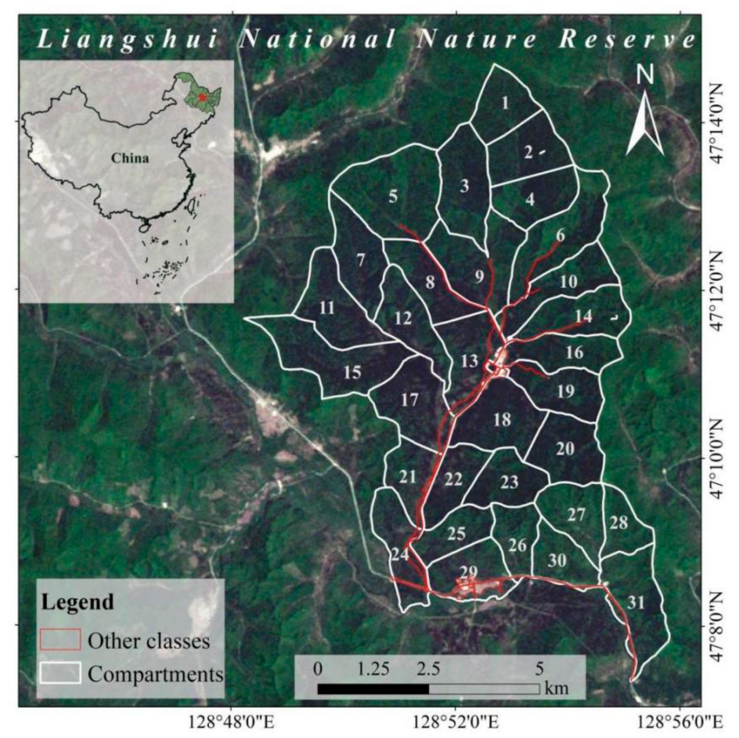
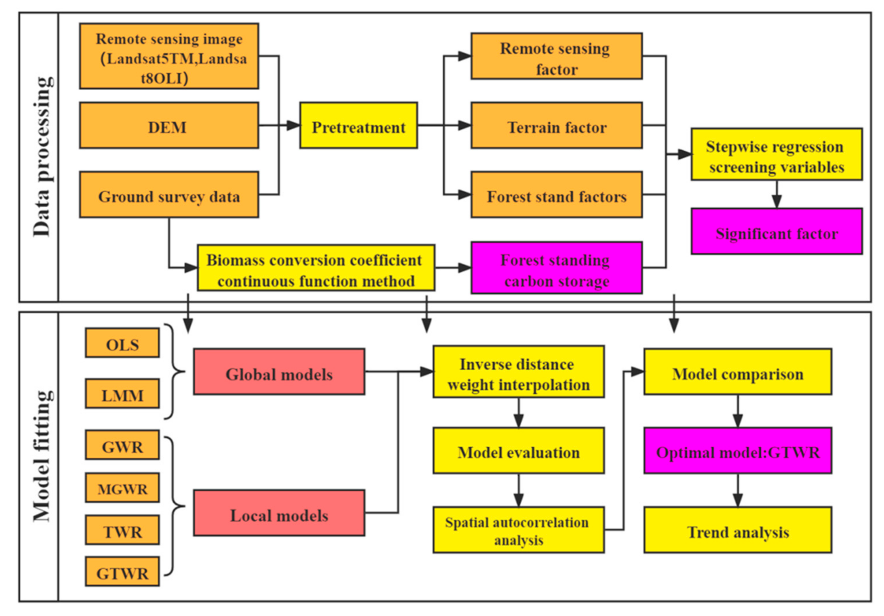
2.1. Study Area and Research Process

The Heilongjiang Liangshui National Nature Reserve is located in Dailing town, Daqingshan County, southeast of Yichun city. The geographical coordinates are 128°53′20″ East longitude and 47°10′50″ North latitude. The total area of the reserve is 12,133 ha: the buffer area is 5739 ha, and the core area is 6394 ha [20]. The specific geographical location and distribution range are shown in Figure 1.

The forest vegetation includes artificially planted red pine, larch, mixed coniferous, broad-leaved, and spruce trees. The natural trees include Korean pine, fir, birch, spruce, mixed coniferous, broad-leaved, soft broad-leaved mixed, hard broad-leaved, and other tree types. The area is rich in natural resources and complex and diverse vegetation community types. It is a representative temperate primitive Korean pine coniferous and broad-leaved mixed forest area in China and Northeast Asia. The complex ecological environment conditions have created very favorable conditions for the survival and reproduction of wild animals and plants. After years of construction and management, the reserve has become a natural base for the protection and research of the ecosystem and biodiversity of Korean pine coniferous and broad-leaved mixed forest in China [21]. The reserve includes 5 species of national secondary key protected wild plants: Pinus koraiensis Siebold & Zucc., Fraxinus mandschurica Rupr., Phellodendron amurense Rupr., Tilia amurensis Rupr., and Glycine soja Siebold & Zucc.; additionally, there is one endemic species: Saliix daikiingensis Chouet King [22].

The main content of the research is shown in Figure 2, which can be divided into two parts: data processing and model fitting. First, the collected remote sensing data are preprocessed, the prediction factors required for the experiment are extracted, and the ground survey data and empirical models are used to calculate carbon storage. The significant factors related to carbon storage are screened out through stepwise regression; then, in the model fitting part, the carbon storage and the screened significant factors are modeled, the fitting effect of the global model and the local model is evaluated, and the intuitive distribution map of carbon storage observation data and model fitting results obtained by interpolation in ArcGIS 10.7 (ESRI, Redlands, CA, USA) [8,14] with the inverse distance weighting method (IDW). The spatial autocorrelation is analyzed by comparing the residual Moran’s I and Z-score of different models under different bandwidths. Finally, the space analysis and error analysis of the optimal model are carried out.

2.2. Data Sources

2.2.1. Ground Survey Data

The ground survey data are from the sample plot data obtained in the Forest Management Inventory in 1989, 1999, 2009, and 2019, including data from 63 sample plots in 1989, 65 sample plots in 1999, 121 sample plots in 2009, and 129 sample plots in 2019. All monitoring plots are evenly distributed in the study area, the plot area is 0.06 ha, and the shape is round or square. During the survey in 1989 and 1999, the locations of the monitored sample plots were the same, and the number of sample plots was basically the same. In the survey in 2009, the number and location of sample plots different from those in 1989 and 1999 were selected. The number and location of sample plots in 2019 are different from those in 1989, 1999, and 2009. Figure 3 shows the distribution of sample sites in different years. In 1989 and 1999, due to the limitations of manpower, material resources, and natural conditions, there were fewer sample sites, but it was still guaranteed that each forest class had at least 1–2 monitoring sites. This also ensures the reliability of the experimental design; the number of monitoring plots nearly doubled in 2009 and 2019, and they were regularly distributed in the study area.

The ground survey data included the geographic location and topographic characteristics of each plot, and records included the number of species, number of trees, diameter at breast height, dominant wood diameter at breast height, and height of all standing trees in the plot. Forest stand factors were calculated per hectare and included storage volume (m³/ha) and carbon storage (Mg/ha). Carbon storage (Mg/ha) was calculated based on the aboveground biomass in the study area using the continuous function method for the biomass conversion coefficient of the main stand types [23]. The calculated biomass was multiplied by the carbon content coefficient to obtain carbon storage [24]. The carbon storage conversion coefficients of different tree species in the study area are shown in

Table 1. Carbon storage conversion coefficients of different tree species in the study area.

Species	Betula platyphylla Suk.	Ulmus pumila L.	Tilia amurensis Rupr.	Quercus mongolica Fisch. ex Ledeb	Picea asperata Mast.	Larix gmelinii (Rupr.) Kuzen.	Pinus koraiensis Sieb. et Zucc.
Conversion coefficients	0.4656	0.4331	0.4373	0.453	0.4805	0.4674	0.4809

:

2.2.2. Remote Sensing Data

The data sources in this paper are Landsat 5 TM data in Liangshui Nature Reserve in 1989, 1999, and 2009 and Landsat 8 OLI data in 2019 [25]. All image resolutions are 30 m. The band characteristics of Landsat 5 TM and Landsat 8 OLI sensors are basically the same, and there is a high degree of consistency in spectral resolution. There is a high degree of consistency in the spectral resolution of these products [26]. In this study, four images with serial number 117,027 at four different points in time were assessed to find the image least influenced by cloud cover. To improve the use quality of remote sensing images, the image was first preprocessed using ENVI 5.3 (Exelis VIS Company, Tysons Corner, VI, USA) [27] to conduct radiometric calibration, atmospheric correction, and geometric correction to eliminate the influence of sunlight and atmosphere on the data; then, the original waveband, vegetation index, and other remote sensing factors were extracted. The indices and corresponding formulas are shown in

Table 2. Vegetation indices and formulas (Landsat 8 OLI).

Vegetation Index	Formula
Blue	B2
Green	B3
Red	B4
Near Infrared	B5
Ratio Vegetation Index (RVI)	$B5/B4$
Difference Vegetation Index (DVI)	$B5-B4$
Weighted Difference Vegetation Index (WDVI)	$B5-0.5\times B4$
Infrared Percentage Vegetation Index (IPVI)	$B5/(B5+B4)$
Perpendicular Vegetation Index (PVI)	$\sin (45°)\times B5-\cos (45°)\times B4$
Normalized Difference Vegetation Index (NDVI)	$(B5-B4)/(B5+B4)$
Transformed Normalized Difference Vegetation Index (TNDVI)	${[(B5-B4)/(B5+B4)+0.5]}^{1/2}$
Soil-Adjusted Vegetation Index (SAVI)	$1.5\times (B5-B4)/8\times (B5+B4+0.5)$
Modified Soil-Adjusted Vegetation Index (MSAVI)	$\begin{array}{l}(2-\mathrm{NDVI}\times \mathrm{WDVI})\times (B5-B4)/\\ 8\times (B5+B4+1-\mathrm{NDVI}\times \mathrm{WDVI})\end{array}$
Modified Soil-Adjusted Vegetation Index 2 (MSAVI2)	$\begin{array}{l}0.5\times (2\times (B5+1))-sqrt[(2\times B5+1)\\ \times (2\times B5+1)-8\times (B5-B4)]\end{array}$
Atmospheric Ratio Vegetation Index (ARVI)	$[B5-(2\times B4-B2)]/[B5+(2\times B4-B2)]$

B2, B3, B4, and B5 are the multispectral bands of remote sensing images.

.

The texture feature of remote sensing images is mainly a visual feature that reflects the homogeneous phenomenon in the image. It reflects the slowly changing or periodically changing surface structure and arrangement properties of the object surface [28]. ENVI 5.3 software was used to calculate the texture features of the original bands. B2, B3, B4, and B5 are the original bands. The texture features include Mean, Variance, Homogeneity, Contract, Dissimilarity, Entropy, Second moment, and Correlation. B3-Mean can be expressed as Mean in B3. Similarly, B4-Mean is Mean in B4 and B4-Entropy is Entropy in B4.

Terrain factors were extracted with a digital elevation model (DEM). DEM is a digital simulation of terrain surfaces or a digital representation of terrain surface morphology created with limited terrain elevation information [29]. ArcGIS 10.7 was used to process the DEM over four years, and terrain factors such as elevation (m) and slope (°) were extracted.

To study the relationships among forest stand factors, topographic factors, remote sensing factors, and carbon storage in the study area, SAS software was used; seven significant factors were identified: Slope, Age, DBH, RVI, B3-Mean, B4-Mean, and B4-Entropy. Figure 4 shows the spatial distribution of variables in different years.

2.3. Methods

2.3.1. Global OLS Model and LMM

OLS regression has been widely used in various studies [30,31]. This experiment uses OLS regression as a benchmark, and the formula is as follows:

$$\mathit{Y}=\beta \mathit{X}+\epsilon$$

(1)

where β is a model coefficient estimated from the data and ε is the model residual, which obeys an N(0, σ²) distribution.

The linear mixed model is extended to the least squares model [32], and the resulting manifestation is as follows:

$$\mathit{Y}=\beta \mathit{X}+\mathit{Zy}+\epsilon$$

(2)

where Y is the vector of the dependent variable, X is the fixed-effect parameter matrix, which is the model coefficient vector of unknown fixed effects, Z is the undetermined random effect matrix, y is the unknown random-effect coefficient vector, and ε is the random error.

The OLS regression assumptions are applied from a regional perspective, making it a fixed-effect model for the dependent variable; in contrast, the LMM considers random effects [33], resulting in a better fitting effect.

2.3.2. Spatial Local Models (GWR, MGWR, TWR and GTWR)

The geographically weighted regression model is based on an expansion of the ordinary global regression model. The spatial influence is considered in model construction in the form of distance weighting [34]. The basic form of the geographically weighted regression model is as follows:

$${\mathit{Y}}_{\mathit{i}}{=\beta }_0{(\mathit{u}}_{\mathit{i}}{, \mathit{v}}_{\mathit{i}})+{\displaystyle \sum }_{\mathit{k}=1}^{\mathit{p}}{\beta }_{\mathit{k}}{(\mathit{u}}_{\mathit{i}}{, \mathit{v}}_{\mathit{i}}{)\mathit{x}}_{\mathit{ik}}{+\epsilon }_{\mathit{i}}, \mathit{i}=1, 2\cdots , \mathit{n}$$

(3)

where ${\mathit{Y}}_{\mathit{i}}$ is the status index of the dependent variable; ${(\mathit{u}}_{\mathit{i}}{, \mathit{v}}_{\mathit{i}})$ are the coordinates of the first sampling point (such as latitude and longitude, or projected coordinates); ${\beta }_{\mathit{k}}{(\mathit{u}}_{\mathit{i}}{, \mathit{v}}_{\mathit{i}})$ is the k-th regression parameter at the i-th sampling point, which is a function of geographic location; ${\epsilon }_i$ is the error term, where ${\epsilon }_{\mathit{i}}$~N(0, σ²); and p is the total number of parameters to be estimated.

In this model, the regression parameters for each sample site are different and can be determined by using the spatial distance weight function method [35]; the basic form is as follows:

$${\hat{\beta }=(\mathit{X}}^{\mathit{T}}{\mathit{W}}_{\mathit{i}}{\mathit{X})}^{-1}{\mathit{X}}^{\mathit{T}}{\mathit{W}}_{\mathit{i}}\mathit{Y})$$

(4)

$${\mathit{W}}_{\mathit{i}}{=\mathit{diag}(\mathit{W}}_{\mathit{i}0}{,\mathit{W}}_{\mathit{i}1}{,\mathit{W}}_{\mathit{i}2}{, \text{…}, \mathit{W}}_{\mathit{in}})$$

(5)

where ${\mathit{W}}_{\mathit{i}}$ is the diagonal matrix of spatial weights for point i, X is the independent variable matrix, Y is the dependent variable matrix, and the superscript T represents matrix transpose.

To solve the parameter estimation problem of GWR, the spatial weight matrix must be appropriately defined; that is, the spatial weight function must be appropriately selected. Generally, the widely used Gaussian function is used [36], and its basic form is:

$${\mathit{W}}_{\mathit{ij}}{=\mathit{exp}(-(\mathit{d}}_{\mathit{ij}}{/\mathit{b})}^2)$$

(6)

where b is bandwidth and is a nonnegative attenuation parameter used to express the functional relationship between weight and distance. If the bandwidth is too small or too large, the fitting accuracy will be affected. Therefore, in the process of model fitting, the bandwidth should be continuously assessed to determine the best bandwidth. Some commonly used bandwidth determination methods include cross-validation (CV), the Akaike criterion (AIC) method and the Bayesian information criterion (BIC) method. In this study, the commonly used quadratic kernel function and the modified Akaike information criterion (AICc) are used to determine the optimal bandwidth [37].

Compared with the traditional GWR, MGWR includes three important improvements. First, the spatial smoothing level of each variable differs [38]. Second, the specific bandwidth of each variable can be used as an indicator of the spatial scale of each spatial process [15]. Third, the multi-bandwidth method produces a more realistic and useful spatial process model than does the traditional method.

The formula for the MGWR model is as follows:

$${\mathit{Y}}_{\mathit{i}}{=\beta }_0{(\mathit{u}}_{\mathit{i}}{, \mathit{v}}_{\mathit{i}})+{\displaystyle \sum }_{\mathit{j}=1}^{\mathit{k}}{\beta }_{\mathit{bwj}}{(\mathit{u}}_{\mathit{i}}{, \mathit{v}}_{\mathit{i}}{)\mathit{X}}_{\mathit{ij}}{+\epsilon }_{\mathit{i}}$$

(7)

where ${(\mathit{u}}_{\mathit{i}}{, \mathit{v}}_{\mathit{i}})$ are the center coordinates of location i; ${\mathit{Y}}_{\mathit{i}}$ is the carbon storage at i, bwj represents the bandwidth associated with the regression coefficient of the fourth variable; ${\beta }_{\mathit{bwj}}{(\mathit{u}}_{\mathit{i}}{, \mathit{v}}_{\mathit{i}})$ is the regression coefficient of variable j at i; and ${\beta }_0{(\mathit{u}}_{\mathit{i}}{, \mathit{v}}_{\mathit{i}})$ and ${\epsilon }_{\mathit{i}}$ are the intercept and error terms of the model, respectively.

Similar to those in the classic GWR model, each regression coefficient in the MGWR model is based on the kernel function and bandwidth selection criteria obtained by local regression [39]. The largest difference between the MGWR model and the classic GWR model lies in the heterogeneity of bandwidth. This improvement is achieved by redefining GWR as a generalized additive model (GAM) [40]. For GAM, a backward fitting algorithm can be used to combine the various smoothing terms. The algorithm first needs to initialize all the smoothing terms. In this study, the classic GWR estimation approach is used to obtain the initial estimate [14,15]. Then, the difference between the true value and the predicted value obtained based on the initial estimate can be calculated as the initialization residual.

$$\hat{\epsilon }=\mathit{Y}-{\displaystyle \sum }_{\mathit{j}=1}^{\mathit{k}}{\hat{\mathit{f}}}_{\mathit{j}}{(\mathit{f}}_{\mathit{j}}{=\beta }_{\mathit{bwj}}{\mathit{X}}_{\mathit{j}})$$

(8)

Next, the residual $\hat{\epsilon }$ is combined with the first additive term ${\mathit{f}}_1$ and the first independent variable X₁ to perform classic GWR and find the optimal bandwidth 1 and a list of new parameter estimates ${\mathit{f}}_1$ and $\hat{\epsilon }$ to update the previous estimates. In the second step, the residual, the second additive term ${\mathit{f}}_2$ and the second independent variable X₂ are used to perform a second round of GWR and update the parameter estimates for the second variables ${\mathit{f}}_2$ and $\hat{\epsilon }$. This process is repeated until the k-th step calculation is completed for the last independent variable X_k. The above steps form a complete loop process and are repeated until the estimate converges to the selected criterion.

The GTWR model includes a temporal dimension, so the coefficients of the local regression equation are a function of geographic location and time scale; this approach enhances analyses of the spatiotemporal characteristics of the regression relationship [18]. The model formula is as follows:

$${\mathit{Y}}_{\mathit{i}}{=\beta }_0{(\mathit{u}}_{\mathit{i}}{, \mathit{v}}_{\mathit{i}}{, \mathit{t}}_{\mathit{i}})+{\displaystyle \sum }_{\mathit{k}=1}^{\mathit{p}}{\beta }_{\mathit{k}}{(\mathit{u}}_{\mathit{i}}{, \mathit{v}}_{\mathit{i}}{,)\mathit{x}}_{\mathit{ik}}{+\epsilon }_{\mathit{i}}, \mathit{i}=1, 2\cdots , \mathit{n}$$

(9)

where ${(\mathit{u}}_{\mathit{i}}{, \mathit{v}}_{\mathit{i}}{, \mathit{t}}_{\mathit{i}})$ are the space-time three-dimensional coordinates of the i-th sample point, n is the number of sample points, ${\epsilon }_{\mathit{i}}$ is the random error associated with the first sample point, ${\epsilon }_{\mathit{i}}$~N(0, σ2), the random errors at sample points i and j are independent of each other, and the covariance is 0. The added parameter represents the observation time of the variable, and ${\beta }_{\mathit{k}}{(\mathit{u}}_{\mathit{i}}{, \mathit{v}}_{\mathit{i}}{, \mathit{t}}_{\mathit{i}})$ is the regression coefficient of the first independent variable for the first sample point [41], which can be expressed as:

$${\hat{\beta }(\mathit{u}}_{\mathit{i}}{, \mathit{v}}_{\mathit{i}}{, \mathit{t}}_{\mathit{i}}{)=(\mathit{X}}^{\mathit{T}}{\mathit{W}(\mathit{u}}_{\mathit{i}}{, \mathit{v}}_{\mathit{i}}{, \mathit{t}}_{\mathit{i}}{\left)\mathit{X}\right)}^{-1}{\mathit{X}}^{\mathit{T}}{\mathit{W}(\mathit{u}}_{\mathit{i}}{, \mathit{v}}_{\mathit{i}}{, \mathit{t}}_{\mathit{i}}\left)\mathit{Y}\right)$$

(10)

In this study, the Gaussian kernel function is used as the space-time weight function of the GTWR model, and the space-time distance is defined as follows:

$${\mathit{d}}_{\mathit{ij}}^{\mathit{ST}}=\sqrt{\lambda \left[{{(\mathit{u}}_{\mathit{i}}-{\mathit{u}}_{\mathit{j}})}^2{+(\mathit{v}}_{\mathit{i}}-{\mathit{v}}_{\mathit{j}}{)}^2\right]{+\mu (\mathit{t}}_{\mathit{i}}-{\mathit{t}}_{\mathit{j}}{)}^2}$$

(11)

where $\lambda$ and $\mu$ are scale factors of spatial and temporal distance, respectively. According to the above definition, and referring to the form of the Gaussian kernel function, the space-time weight function can be obtained as follows:

$${\mathit{w}=(\mathit{u}}_{\mathit{i}}{, \mathit{v}}_{\mathit{i}}{, \mathit{t}}_{\mathit{i}})=\exp (-\frac{{\mathit{d}}_{\mathit{ij}}^{\mathit{ST}}}{{\mathit{h}}^2})=\exp \left\{-\frac{\lambda \left[{{(\mathit{u}}_{\mathit{i}}-{\mathit{u}}_{\mathit{j}})}^2{+(\mathit{v}}_{\mathit{i}}-{\mathit{v}}_{\mathit{j}}{)}^2\right]{+\mu (\mathit{t}}_{\mathit{i}}-{\mathit{t}}_{\mathit{j}}{)}^2}{{\mathit{h}}^2}\right\}$$

(12)

where h is the bandwidth function, and the optimal bandwidth is determined by the AICc. When the scale factor $\mu$ is 0, only the spatial distance and spatial heterogeneity are considered in the GWR model; when the scale factor $\lambda$ is 0, only the temporal distance and temporal nonstationarity are considered, and a temporally weighted regression (TWR) model is established.

2.3.3. Model Evaluation

This article uses five statistics to evaluate the effect of model fitting: the residual sum of squares (RSS), root mean square error (RMSE), AICc value, correlation coefficient (R²), and adjusted correlation coefficient (${\mathit{R}}_{\mathit{a}}^2$). Moran’s I and Z-score were used to evaluate the spatial autocorrelation of the residuals of each model. The sum of each squared residual is called the residual sum of squares (RSS), which represents the effect of random error. The smaller the RRS of a set of data is, the better the fit. The corresponding expression is as follows:

$$\mathrm{RSS}={\displaystyle \sum }_{i=1}^n{{(\mathit{y}}_{\mathit{i}}-\widehat{{\mathit{y}}_{\mathit{i}}})}^{2 }$$

(13)

where ${\mathit{y}}_{\mathit{i}}$ and $\widehat{{\mathit{y}}_{\mathit{i}}}$ are the observed and predicted values of the dependent variable and $\mathit{n}$ is the sample size.

The root mean square error (RMSE) is used as the statistic for independence tests. The RMSE is also used to measure the deviation between an estimated value and the true value. The lower the RMSE is, the better the fitting ability of the model. The RMSE is expressed as follows:

$$\mathrm{RMSE}=\sqrt{\frac{{{\displaystyle \sum }}_{\mathit{i}=1}^{\mathit{n}}{(\mathit{y}}_{\mathit{i}}-\widehat{{\mathit{y}}_{\mathit{i}}})}{\mathit{n}}}$$

(14)

where ${\mathit{y}}_{\mathit{i}}$ and $\widehat{{\mathit{y}}_{\mathit{i}}}$ are the observed and predicted values of the dependent variable and $\mathrm{n}$ is the sample size.

AICc is one of the most commonly used goodness-of-fit standards in model comparison. The smaller the AICc is, the better the model performance. The corresponding formula is as follows:

$$\mathrm{AICc}=\mathit{ln}\frac{\mathrm{RSS}}{\mathit{n}}+\frac{\mathit{n}+\mathit{k}}{\mathit{n}-\mathit{k}-2}$$

(15)

where n is the sample size, k is the number of parameters in the fitted model, and RSS is the residual sum of squares.

The correlation coefficient (R²) represents the goodness of fit of a model, or the percentage of the total change in the observations explained by the model. The larger R² is, the better the model fitting result. R² tends to exaggerate the explained percentage because it is not reduced by adding more predictors [42]. The adjusted coefficient of determination (${\mathit{R}}_{\mathit{a}}^2$) overcomes this shortcoming by dividing the RSS and SST by their related degrees of freedom, and the corresponding formulas are as follows:

$${\mathit{R}}^2=1-\frac{\mathrm{RSS}}{\mathrm{SST}}$$

(16)

$${\mathit{R}}_{\mathit{a}}^2{=1 - (1 - \mathit{R}}^2) \times \frac{\mathit{n}-1}{\mathit{n}-\mathit{k}-1}$$

(17)

where RSS is the residual sum of squares, SST is the total sum of squares, n is the number of samples, and k is the number of parameters in the fitted model.

Moran’s I is typically used to investigate the spatial autocorrelation of model residuals among regression models [43]. When the model residuals tend to be similar, Moran’s I is positive; when the model residuals tend to be different, Moran’s I is negative; and when the model residuals are arranged randomly and independently in space, Moran’s I is approximately 0. This index can be expressed as:

$$\mathrm{I}=\frac{\mathit{n}}{{\mathit{S}}_0}\times \frac{{{\displaystyle \sum }}_{\mathit{i}=1}^{\mathit{n}}{{\displaystyle \sum }}_{\mathit{i}=1}^{\mathit{n}}{\mathit{w}}_{\mathit{ij}}{(\mathit{c}}_{\mathit{i}}-\overline{\mathit{c}})({\mathit{c}}_{\mathit{j}}-\overline{\mathit{c}})}{{{\displaystyle \sum }}_{\mathit{i}=1}^{\mathit{n}}{{(\mathit{c}}_{\mathit{i}}-\overline{\mathit{c}})}^2}{\mathit{w}}_{\mathit{ij}}$$

(18)

where ${\mathit{w}}_{\mathit{ij}}$ is the spatial weight between elements i and j, n is the total number of samples, ${\mathit{c}}_{\mathit{i}}$ is the residual at i, $\overline{\mathit{c}}$ is the average of the residuals, and ${\mathit{S}}_0$ is the aggregation of all spatial weights:

$${\mathit{S}}_0={\displaystyle \sum }_{\mathit{i}=1}^{\mathit{n}}{\displaystyle \sum }_{\mathit{i}=1}^{\mathit{n}}{\mathit{w}}_{\mathit{ij}}$$

(19)

The Z-score is a multiple of the standard deviation and can effectively reflect the degree of dispersion of a data set [16]. The statistical Z-score formula is as follows:

$$\mathrm{Z}=\frac{\mathrm{I}-\mathit{E}\left(\mathrm{I}\right)}{\sqrt{\mathit{V}\left(\mathrm{I}\right)}}$$

(20)

$$\mathit{E}\left(\mathrm{I}\right)=\frac{-1}{\mathit{n}-1}$$

(21)

$${\mathit{V}\left(\mathrm{I}\right)=\mathit{E}(\mathrm{I}}^2{) - \mathit{E}(\mathrm{I})}^2$$

(22)

If the Z-score is between −1.96 and +1.96, the uncorrected p value will be greater than 0.05, so the null hypothesis cannot be rejected because the displayed pattern is likely to be the result of a random spatial process, such as spatial autocorrelation. If the Z-score is less than −2.58 or greater than +2.58, the observed spatial pattern may be extremely uncommon and may not be the result of a random process; a small p value can also reflect this result, indicating strong spatial autocorrelation [16,19].

3. Results

3.1. Comparison of Model Fitting Results

The fitting results of all models are shown in

Table 3. Comparison of the fitting results of the OLS, LMM, GWR, MGWR, TWR, and GTWR models.

Model	RSS	RMSE	AICc	R2	${\mathit{R}}_{\mathit{a}}^2$
OLS	889,784	48.52	4026	0.464	0.454
LMM	778,693	45.39	3995	0.527	0.519
GWR	710,468	43.35	3989	0.572	0.536
MGWR	681,806	42.47	3988	0.589	0.547
TWR	594,131	39.65	3953	0.643	0.637
GTWR	443,198	34.24	3912	0.734	0.729

. With the OLS global model, the fitting effect is relatively moderate, the AICc value of all models is the largest, and ${\mathit{R}}_{\mathit{a}}^2$ is the smallest. The LMM outperforms the OLS model when random effects are added. GWR and MGWR consider the spatial factors of the study area, and the fitting effect is better than that of the former two modes. TWR introduces a temporal factor into the model, and the model performance is second only to that of GTWR. GTWR yields the best fitting effect, with the smallest AICc value and largest ${\mathit{R}}_{\mathit{a}}^2$. The RSS, MSE, and RMSE of GTWR are also reflective of good performance.

Figure 5 shows the carbon storage observation data and model fitting results for the Liangshui Nature Reserve in different years, obtained by interpolation in ArcGIS 10.7 with the IDW. The geographic locations of the sample plots monitored during the second-class surveys in 1989 and 1999 were the same. The number of sample plots was also basically the same; therefore, the carbon storage distribution in the two years was roughly similar, but carbon storage varied in different parts of the reserve. The northernmost, westernmost and southernmost areas exhibited the highest carbon storage, ranging from 120 to 180 (Mg/ha). The central area displayed scattered regions of high carbon storage, with carbon storage ranging from 80 to 120 (Mg/ha). Carbon storage in most other regions ranged from 20 to 60 (Mg/ha). In the survey in 2009, a different number of plots than that in 1989 and 1999 was selected, and new plot locations were selected. In addition, the natural tree growth and windfall results indicated that the distribution of CS slightly differed from 10 and 20 years earlier, but the overall distribution was similar. Similarly, the carbon storage in the west was relatively high, ranging from 120 to 180 (Mg/ha), and the area with high carbon storage in the central region was wide, with values ranging from 160 to 200 (Mg/ha). The carbon storage in the eastern region was relatively low, ranging from 20 to 60 (Mg/ha), and the carbon storage in other regions varied from 60 to 120 (Mg/ha). The total carbon storage was clearly higher than that in 1989 and 1999. In 2019, new sample locations different from 2009 were used in the survey. The general carbon storage distribution was basically the same as that in previous years. Carbon storage increased in the northernmost region of the reserve, the distribution of high-carbon areas broadened, and the total carbon storage increased.

From a temporal perspective, carbon stocks showed an increasing trend from 1989 to 2019. A comparison of the observation results and model results suggests that the estimated results of the global OLS model and LMM are significantly different from the observations in terms of the geographical distribution, and large gaps in carbon storage values exist. The estimated results of the local GWR, MGWR, TWR, and GTWR models are basically consistent with the observation data in terms of distribution, but the carbon storage values obtained with GWR and MGWR are slightly different from the observations; the TWR and GTWR models provide relatively good estimated results. Among them, GTWR yields the best fitting effect, and both the geographical distribution and the value of carbon storage are closest to the observed values. The purpose of making Figure 5 is to make the fitting results look more concrete, and also to use a more intuitive way to show the spatial distribution of the fitting results of different models.

3.2. OLS and LMM

The OLS regression model is used to estimate the relationship between CS and impact factors, and it is used as a benchmark for model comparison. The OLS model is based on a global fixed effect and only reflects the average relationship between the dependent variable and the predictors [44,45]. The LMM adds random effects on the basis of the OLS approach, and the parameter estimation results of the two models are similar.

Table 4. Comparison of parameter estimates with the OLS model and LMM.

Parameter	Estimate		Std. Error		t Test		p Value
	OLS	LMM	OLS	LMM	OLS	LMM	OLS	LMM
Intercept	36.187	47.556	20.306	20.162	1.78	2.36	0.075	0.046
Slope	−2.936	−2.862	0.952	0.942	−3.08	−3.04	0.002	0.016
Age	0.353	0.362	0.091	0.098	3.87	3.7	0.000	0.006
DBH	1.775	1.622	0.259	0.321	6.84	5.06	0.000	0.001
RVI	−3.075	−3.840	1.047	1.016	−2.94	−3.78	0.003	0.005
B3-Mean	8.805	9.2573	1.900	1.808	4.63	5.12	0.000	0.001
B4-Mean	−7.196	−8.077	1.745	1.780	−4.12	−4.54	0.000	0.002
B4-Entropy	11.984	12.415	5.646	5.476	−2.12	−2.27	0.034	0.053

indicates that carbon storage increases as Age, DBH, B3-Mean, and B4-Mean increase, reflecting a positive correlation. Additionally, carbon storage increases as Slope, RVI, B4-Mean, and B4-Entropy decrease, reflecting a negative correlation.

3.3. GWR, MGWR, TWR and GTWR

The GWR and MGWR models take local spatial factors into account and solve spatial heterogeneity problems. The TWR and GTWR models further consider time and simultaneously solve temporal and space heterogeneity problems [46]. The adaptive double-square kernel function is used as the spatial weighting kernel function, and the appropriate bandwidth is selected according to the smallest AICc value [47].

Table 5. Comparison of parameter estimates with the GWR, MGWR, TWR, and GTWR models.

Parameter	Models	Mean	STD	Min	Median	Max
Intercept	GWR	59.122	14.526	31.178	66.296	80.532
	MGWR	42.777	0.363	42.055	42.849	43.510
	TWR	19.721	41.639	−35.698	26.179	66.296
	GTWR	25.408	56.280	−113.552	30.221	196.112
Slope	GWR	−3.425	1.522	−5.925	−3.688	−0.035
	MGWR	−2.017	0.077	−2.081	−2.067	−1.808
	TWR	−3.103	0.425	−3.688	−2.926	−2.736
	GTWR	−2.869	1.615	−7.173	−2.796	2.006
Age	GWR	0.236	0.371	−0.426	0.18	0.912
	MGWR	0.369	0.183	0.034	0.341	1.024
	TWR	0.444	0.296	0.180	0.297	0.922
	GTWR	0.428	0.316	−0.021	0.350	1.182
DBH	GWR	2.264	1.497	0.432	1.469	4.982
	MGWR	1.633	0.035	1.571	1.636	1.694
	TWR	2.219	2.296	−0.256	1.469	5.432
	GTWR	1.810	1.762	−0.764	1.380	6.481
RVI	GWR	−4.889	1.628	−10.281	−4.799	−3.117
	MGWR	−3.166	0.375	−3.734	−3.220	−2.472
	TWR	−1.322	1.482	−3.347	−0.594	0.191
	GTWR	−1.501	5.905	−18.245	−0.324	12.037
B3-Mean	GWR	9.977	2.213	5.484	10.983	11.7
	MGWR	7.227	0.042	7.142	7.225	7.337
	TWR	5.942	4.192	1.951	3.959	11.665
	GTWR	7.328	8.908	−4.139	4.086	34.291
B4-Mean	GWR	−9.94	3.406	−15.417	−10.35	−3.572
	MGWR	−6.508	0.082	−6.613	−6.550	−6.285
	TWR	−5.238	4.067	−10.350	−4.783	−0.395
	GTWR	−9.008	9.704	−40.573	−6.802	5.123
B4-Entropy	GWR	−9.398	4.682	−17.063	−10.178	1.933
	MGWR	−11.405	0.506	−11.962	−11.640	−10.092
	TWR	−4.052	9.373	−11.391	−10.178	9.593
	GTWR	1.475	14.355	−41.318	0.415	36.677

summarizes the parameter estimates of the four models. Except for the median coefficient of B4-Entropy for the GTWR model, the positive and negative median coefficients of all other models are consistent with the positive and negative median coefficients of the OLS model and LMM. Notably, the model parameters of GWR and MGWR are highly similar [48], and the model parameters of TWR are closest to those of GTWR.

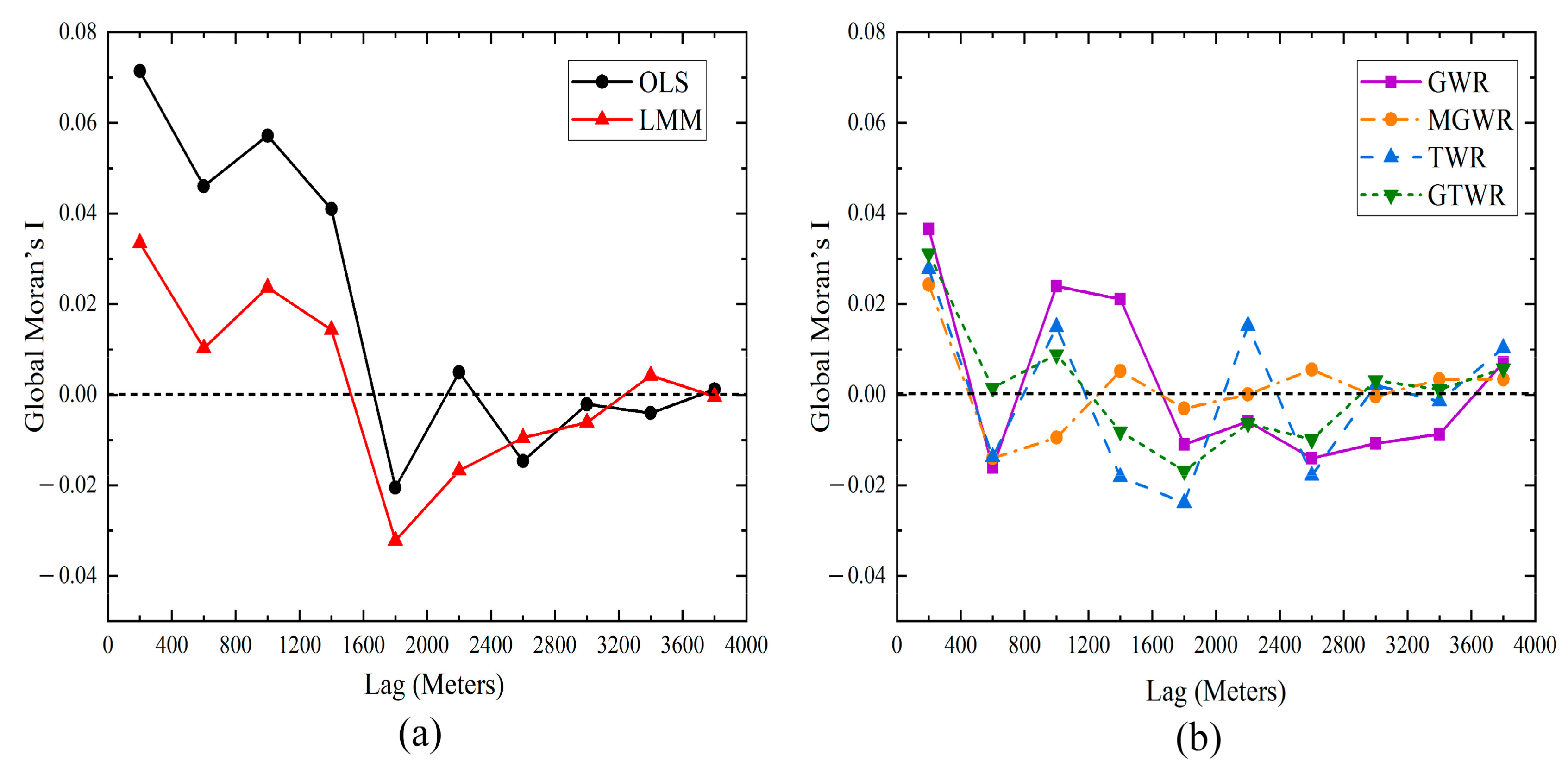
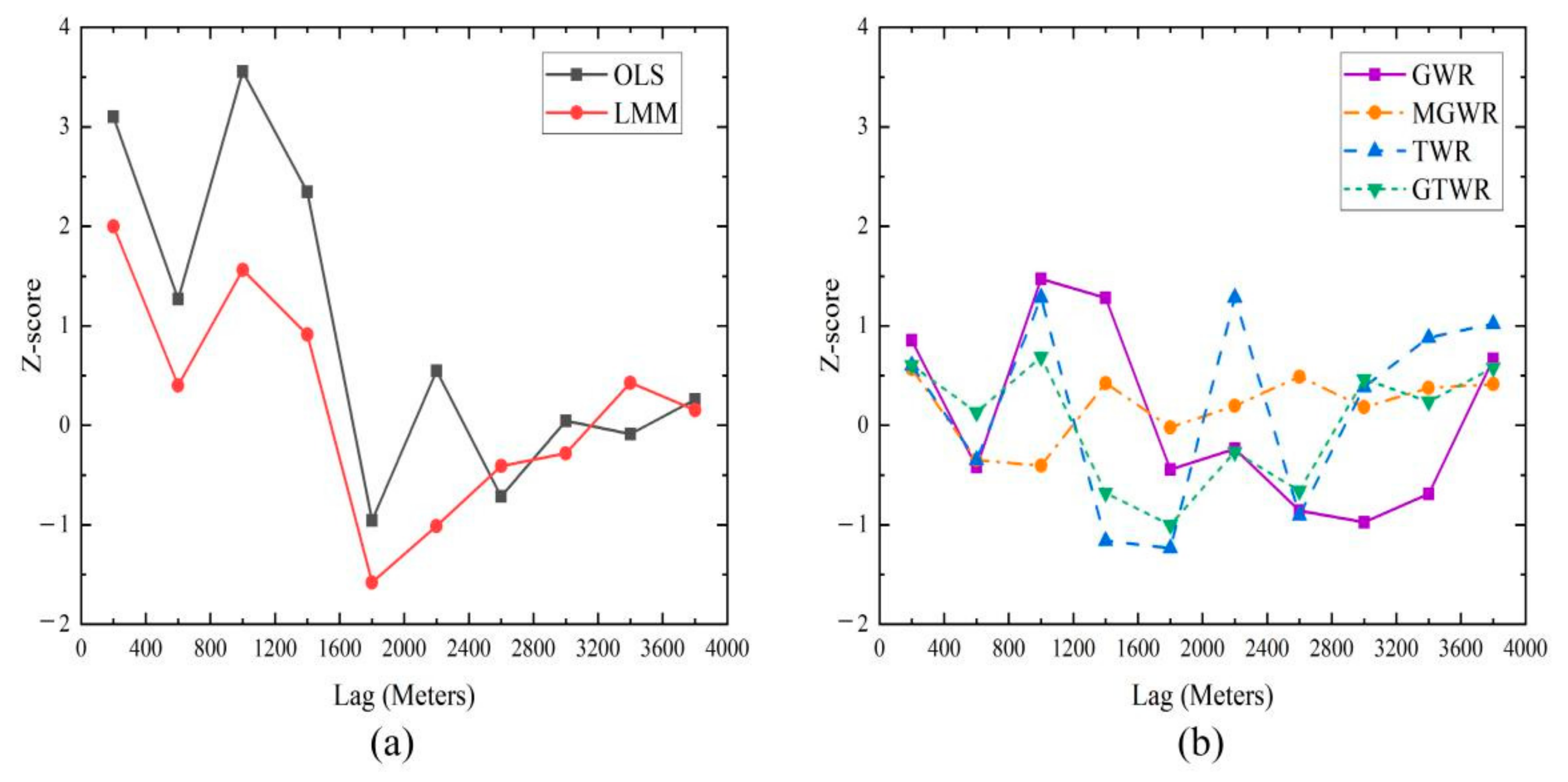
3.4. Spatial Autocorrelation Analysis

In order to study the spatial correlation of residuals of different models, the residual Moran’s I and Z-scores of OLS, LMM, GWR, MGWR, TWR, and GTWR models at 10 different bandwidths from 0 m to 4000 m are calculated and compared. Figure 6 shows the variation trend of Moran’s I of the global model residual at different bandwidths. Notably, the Moran’s I trends of the OLS model and LMM residuals are roughly the same. The spatial autocorrelation associated with the LMM residuals is greatly reduced, but the Moran’s I values of the model residuals at a small spatial scale (0–1200 m) are still very large. As the spatial scale becomes increasingly larger, Moran’s I of the residuals of the two models approaches 0, which means that the spatial autocorrelation decreases with increasing scale [49]. The residual Moran’s I values of the local GWR, MGWR, TWR, and GTWR models are much smaller than that of the global OLS model, the degree of spatial autocorrelation is low, and there is a general negative correlation between the residuals. At small spatial scales, the Moran’s I values of the residual of the GWR (0–400 m and 800–1200 m) model are larger than those of other models [50]; additionally, the Moran’s I values of the residuals of the MGWR model at all scales are closest to 0, and the Moran’s I trends of the residuals of the TWR and GTWR models are the same, but the GTWR residuals are closer to 0 than those of TWR at each spatial scale.

Figure 7 shows the Z-score of the residuals of each model. When the scale of the OLS model is 0–400 m and 800–1200 m, the Z-scores are 3.1 and 3.6, respectively, which are both greater than 2.58. This finding indicates that the residual of the OLS model has a high degree of spatial autocorrelation at small scales. The Z-score of the residual of the LMM is 2, which is greater than 1.96, when the scale is 0–400 m, indicating that there is a certain spatial autocorrelation at this scale. The Z-scores of the GWR, MGWR, TWR, and GTWR model residuals are greater than −2.58 or less than 2.58 at all scales, indicating that the spatial autocorrelation of the residuals of these models is low [15].

By combining the Moran’s I and Z-score results for the residuals of each model, we find that spatial autocorrelation is notable for the OLS model, thus violating the OLS assumptions and leading to biased estimates of coefficients [51]. The LMM overcomes the spatial self-correlation issue to a certain extent, although issues still exist at small scales. Various GWR-based models (GWR, MGWR, TWR, and GTWR) can significantly reduce this spatial autocorrelation issue [52]. MGWR overcomes the influence of spatial autocorrelation to the greatest extent and outperforms the other methods without considering the time dimension. GTWR greatly reduces the spatial autocorrelation while considering time. Thus, for estimations of long-term carbon storage, GTWR is the optimal model [53].

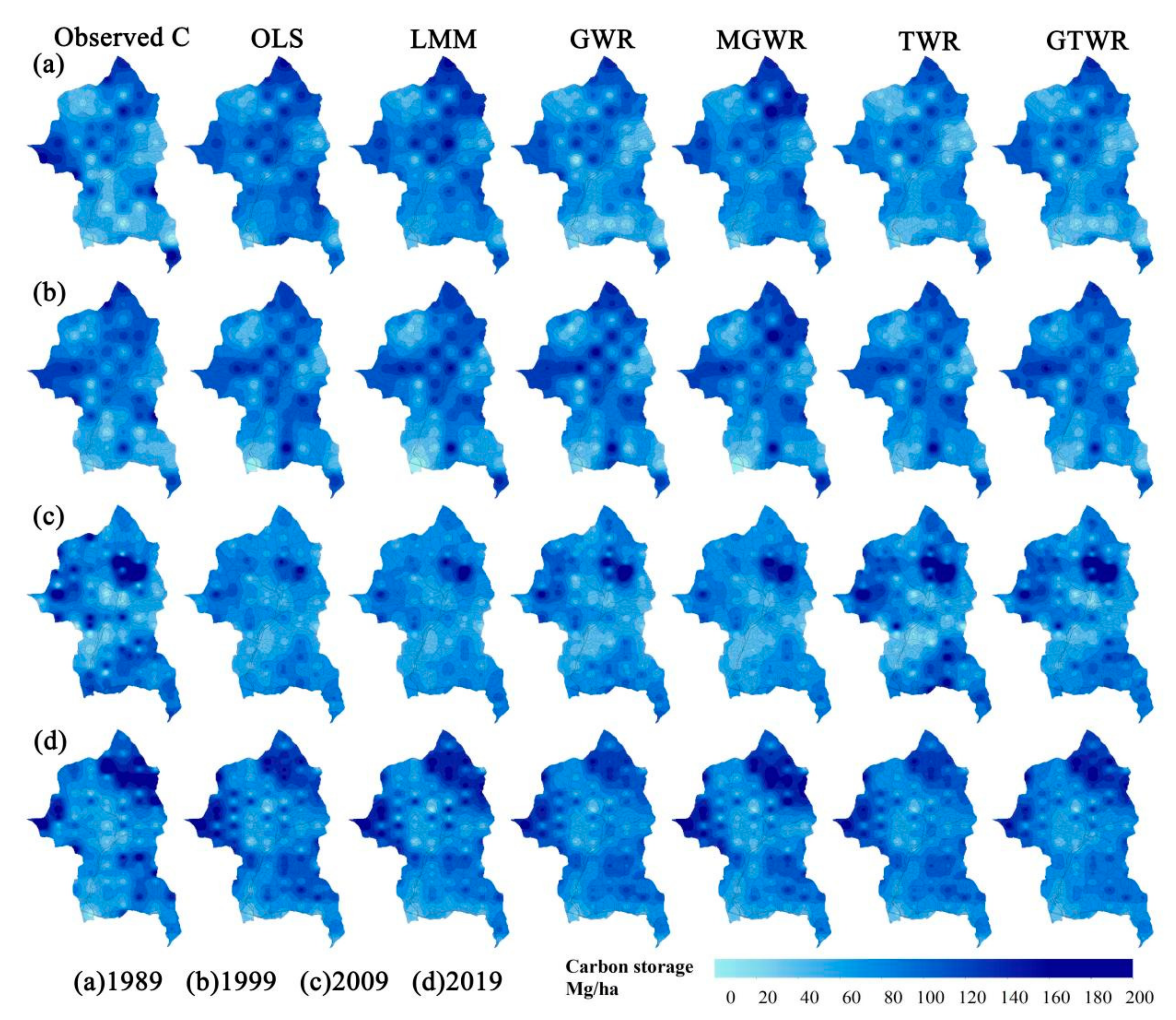
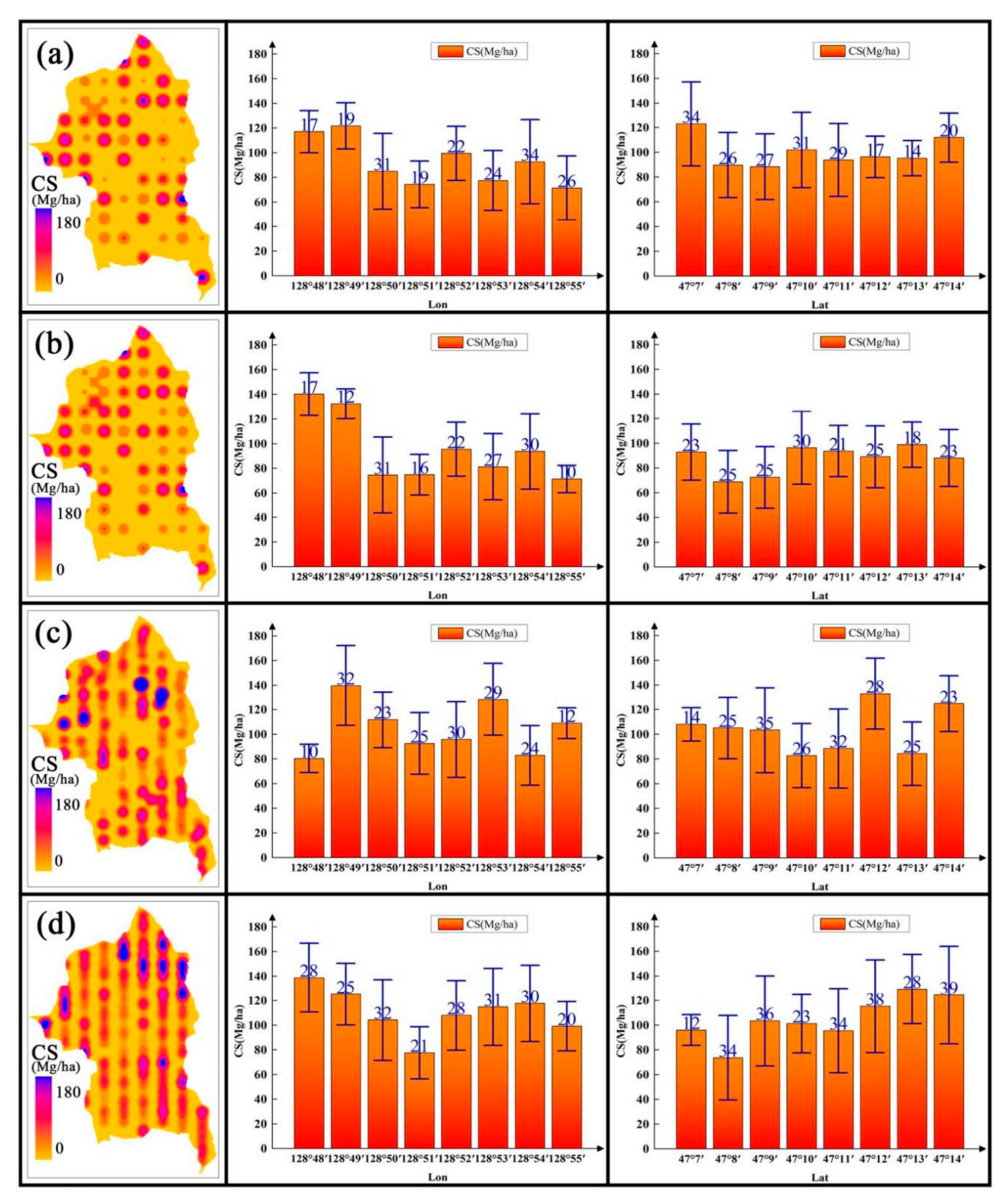
3.5. Optimal Model Space Analysis

Figure 8 shows the carbon storage heat map of standing trees fitted by GTWR model and the error analysis diagram of average carbon storage at different longitudes and latitudes. We can visually see the spatial distribution of carbon in different years. The carbon storage distribution in 1989 and 1999 was roughly similar, with higher carbon reserves in the north and west than in other regions. Carbon storage increased significantly in 2009 and 2019 compared with 1989 and 1999, with those in the north being higher than in other regions; the specific spatial distribution is shown in the figure below. It can also be seen intuitively from the figure that the GTWR model fits the distribution of carbon storage in different longitudes and latitudes and the error range. We find that the GTWR model basically controls the error range within 10–30%, and the fitting effect is good but still has a large room for improvement. How to further improve the fitting effect will be our next work to be studied.

4. Discussion

Northeast China is the region with the richest forest carbon reserves in China, and it includes the Greater Xing’an Mountains, Xiao Xing’an Mountains, and Changbai Mountains. The Liangshui Nature Reserve is located in the southeastern section of the Xiao Xing’an Mountains and on the east slope of the Dali Belt Ridge. Remote sensing images and forest stand survey data were used to study the distribution of carbon storage in the Liangshui area and provide a reference significance for studying the distribution of standing wood carbon storage in the entire northeast region [30]. The Liangshui Nature Reserve, as a natural forest area, is characterized by important strategic significance in terms of a natural ecosystem balance in the context of achieving carbon neutrality. When using stand factor, terrain factor, remote sensing factor, and other data for prediction and carbon storage analysis, a lot of manpower and material resources required for manual census can be saved, and the results provide important reference value for the monitoring of natural ecosystems and establishment of management plans for protected areas [24].

This study uses OLS, LMM, GWR, MGWR, TWR, and GTWR models based on 1989, 1999, 2009, and 2019 two-year survey data, as well as Landsat 5 TM and Landsat 8 OLI data, to investigate the distribution of standing wood carbon storage in forests in the Liangshui Nature Reserve. Notably, carbon storage is heterogeneous in space and time. The OLS model can predict standing wood carbon storage to a certain extent, but the global model assumes the carbon process to be constant in time and space. Thus, spatial and temporal heterogeneity may cause biased estimates of model coefficients [54]. The LMM is also a global model, but it considers random effect errors to address spatial and temporal autocorrelation issues, thus producing a better fitting effect than that of the OLS approach (${\mathit{R}}_{\mathit{a}}^2$ increased by 14%) [55]. The local GWR and MGWR models include geographic location information and can overcome spatial heterogeneity issues; additionally, these models outperform the OLS model and LMM [56]. Notably, MGWR is based on a multi-bandwidth method and produces a realistic and useful spatial result [57]. The Moran’s I of the residuals of the MGWR model is the smallest among those of all models at different bandwidths, indicating that the impact of spatial autocorrelation is highly mitigated. If time is not considered, the MGWR model exhibits the best performance; that is, MGWR is fully capable of assessing the spatial distribution of standing wood carbon storage in short periods or single years. The TWR and GTWR models also include time. As a result, these models perform well [58]; compared with that of the OLS model, the ${\mathit{R}}_{\mathit{a}}^2$ value increases by 40% and 61%, respectively, for these models. When TWR only introduces temporal distance and temporal nonstationarity, the performance of the model is better than that of MGWR, indicating that in assessments of the distribution of long-period standing wood carbon storage in forests, temporal nonstationarity is more important than spatial nonstationarity. Of course, this result may be related to the limited number of samples [59]. GTWR includes temporal and spatial factors at the same time, and ${\mathit{R}}_{\mathit{a}}^2$ is 0.729; additionally, the model residuals (RSS and RMSE are the smallest of all models) are the most ideal, and the AICc value is the smallest. These results indicate that, in the studies of the long-term distribution of standing wood carbon storage, the GTWR model has an absolute advantage over other methods. The GTWR model based on survey data from 1989, 1999, 2009, and 2019 can be used to determine the relationship between standing wood carbon storage and stand factors, topographic factors, and remote sensing factors. In particular, the acquisition of data from remote sensing products saves manpower and material resources. It is possible to predict forest standing wood carbon storage to a certain extent without conducting large-scale field surveys, thus promoting the path to carbon neutrality [60]. According to the research results, the GTWR model displays the best performance of the considered models, but the effect of GTWR on spatial heterogeneity is not as good as that of MGWR; thus, determining how this effect can be improved should be a focus of future studies. Another thing to note is that, due to the limited number of samples, the IDW mapping results of these models may not be enough to be evaluated in this study, and high-precision results (airborne data, especially unmanned aerial vehicle LiDAR data) should be used for subsequent verification work [54].

5. Conclusions

In this study, the global and local models were used to study the spatiotemporal distribution of forest carbon storage in the Liangshui Nature Reserve, to compare the fitting effects of different models, and to conduct spatial autocorrelation analysis. The results showed that parameter (Age, DBH and B3-Mean) estimates tended to be positive for predicting standing wood carbon storage, and parameter (RVI, B3-Mean, B4-Mean and B4-Entropy) estimates tended to be negative for predicting standing wood carbon storage. The global model (OLS, LMM) has poor fitting results compared to the local model (GWR, MGWR, TWR, and GTWR), and OLS model yields the worst fitting effect. As a global model, the LMM also has a higher ${\mathit{R}}_{\mathit{a}}^2$ and more ideal model residuals than the OLS model. Notably, ${\mathit{R}}_{\mathit{a}}^2$ is 14% higher than that of the OLS model. The fitting effects of the GWR, MGWR, TWR, and GTWR models are further improved; notably, compared with that of OLS, ${\mathit{R}}_{\mathit{a}}^2$ increased by 18%, 20%, 40%, and 61% with these models, respectively. TWR performs better than GWR and MGWR when only considering temporal factors, indicating that temporal heterogeneity is more influential than spatial heterogeneity. Especially for the long-term monitoring of carbon storage distributions, temporal factors play an important role in model fitting. The traditional OLS model is influenced by strong spatial autocorrelation, which will lead to biased estimates of model coefficients. Although the LMM is an improvement over the OLS approach, it is inferior to the local GWR-based models (GWR, MGWR, TWR, and GTWR). MGWR solves the spatial heterogeneity problem to the greatest extent observed. If time is not considered, MGWR performs best. Considering both temporal heterogeneity and spatial heterogeneity problems, GTWR provides a good fitting effect, and compared with other models in this study, it yields the best ${\mathit{R}}_{\mathit{a}}^2$ and the most ideal model residuals.

This study provides evidence of spatiotemporal heterogeneity between forest carbon storage and forest stand factors, topographic factors, and remote sensing factors in the Liangshui area. Additionally, possible solutions for modeling forest carbon storage and other related factors in the Liangshui area are given. This study contributes to the investigation of ecological resources in protected areas, and the results could be used by relevant departments in the monitoring of carbon storage.

References

1. Wen, D.; He, N. Forest Carbon Storage along the North-South Transect of Eastern China: Spatial Patterns, Allocation, and Influencing Factors. Ecol. Indic. 2016, 61, 960–967. [Google Scholar] [CrossRef]
2. Li, M. Carbon Stock and Sink Economic Values of Forest Ecosystem in the Forest Industry Region of Heilongjiang Province, China. J. For. Res. 2021, 1–8. [Google Scholar] [CrossRef]
3. Guo, Y.T.; Zhang, X.M.; Long, T.F.; Jiao, W.L.; He, G.J.; Yin, R.Y.; Dong, Y.Y. China forest cover extraction based on google earth engine. Int. Arch. Photogramm. Remote Sens. Spat. Inf. Sci. 2020, 42, 855–862. [Google Scholar] [CrossRef] [Green Version]
4. Gundersen, P.; Thybring, E.E.; Nord-Larsen, T.; Vesterdal, L.; Nadelhoffer, K.J.; Johannsen, V.K. Old-Growth Forest Carbon Sinks Overestimated. Nature 2021, 591, E21–E23. [Google Scholar] [CrossRef] [PubMed]
5. Anand, A.; Pandey, P.C.; Petropoulos, G.P.; Pavlides, A.; Srivastava, P.K.; Sharma, J.K.; Malhi, R.K.M. Use of Hyperion for Mangrove Forest Carbon Stock Assessment in Bhitarkanika Forest Reserve: A Contribution towards Blue Carbon Initiative. Remote Sens. 2020, 12, 597. [Google Scholar] [CrossRef] [Green Version]
6. Franki, V.; Višković, A.; Šapić, A. Carbon Capture and Storage Retrofit: Case Study for Croatia. Energy Sources Part A: Recovery Util. Environ. Eff. 2021, 43, 3238–3250. [Google Scholar] [CrossRef]
7. Tao, S.; Guo, Q.; Li, L.; Xue, B.; Kelly, M.; Li, W.; Xu, G.; Su, Y. Airborne Lidar-Derived Volume Metrics for Aboveground Biomass Estimation: A Comparative Assessment for Conifer Stands. Agric. For. Meteorol. 2014, 198–199, 24–32. [Google Scholar] [CrossRef]
8. Hu, T.; Sun, Y.; Jia, W.; Li, D.; Zou, M.; Zhang, M. Study on the Estimation of Forest Volume Based on Multi-Source Data. Sensors 2021, 21, 7796. [Google Scholar] [CrossRef]
9. Takagi, K.; Yone, Y.; Takahashi, H.; Sakai, R.; Hojyo, H.; Kamiura, T.; Nomura, M.; Liang, N.; Fukazawa, T.; Miya, H.; et al. Forest Biomass and Volume Estimation Using Airborne LiDAR in a Cool-Temperate Forest of Northern Hokkaido, Japan. Ecol. Inform. 2015, 26, 54–60. [Google Scholar] [CrossRef]
10. Narmada, K.; Annaidasan, K. Estimation of the Temporal Change in Carbon Stock of Muthupet Mangroves in Tamil Nadu Using Remote Sensing Techniques. JGEESI 2019, 19. [Google Scholar] [CrossRef]
11. Roy Chowdhury, P.K.; Maithani, S. Modelling Urban Growth in the Indo-Gangetic Plain Using Nighttime OLS Data and Cellular Automata. Int. J. Appl. Earth Obs. Geoinf. 2014, 33, 155–165. [Google Scholar] [CrossRef]
12. Krämer, W.; Bartels, R.; Fiebig, D.G. Another Twist on the Equality of OLS and GLS. Stat. Pap. 1996, 37, 277–281. [Google Scholar] [CrossRef]
13. Zhang, L.; Ma, Z.; Guo, L. Spatially assessing model errors of four regression techniques for three types of forest stands. Forestry 2008, 81, 209–225. [Google Scholar] [CrossRef] [Green Version]
14. Hajiloo, F.; Hamzeh, S.; Gheysari, M. Impact Assessment of Meteorological and Environmental Parameters on PM2.5 Concentrations Using Remote Sensing Data and GWR Analysis (Case Study of Tehran). Environ. Sci. Pollut. Res. 2019, 26, 24331–24345. [Google Scholar] [CrossRef]
15. Yu, H.; Fotheringham, A.S.; Li, Z.; Oshan, T.; Kang, W.; Wolf, L.J. Inference in Multiscale Geographically Weighted Regression. Geogr. Anal. 2020, 52, 87–106. [Google Scholar] [CrossRef]
16. Wei, Q.; Zhang, L.; Duan, W.; Zhen, Z. Global and Geographically and Temporally Weighted Regression Models for Modeling PM2.5 in Heilongjiang, China from 2015 to 2018. IJERPH 2019, 16, 5107. [Google Scholar] [CrossRef] [Green Version]
17. Cohen, J.P.; Coughlin, C.C.; Zabel, J. Time-Geographically Weighted Regressions and Residential Property Value Assessment. J. Real Estate Financ. Econ. 2020, 60, 134–154. [Google Scholar] [CrossRef] [Green Version]
18. Fotheringham, A.S.; Crespo, R.; Yao, J. Geographical and Temporal Weighted Regression (GTWR): Geographical and Temporal Weighted Regression. Geogr. Anal. 2015, 47, 431–452. [Google Scholar] [CrossRef] [Green Version]
19. Chu, H.-J.; Bilal, M. PM2.5 Mapping Using Integrated Geographically Temporally Weighted Regression (GTWR) and Random Sample Consensus (RANSAC) Models. Environ. Sci. Pollut. Res. 2019, 26, 1902–1910. [Google Scholar] [CrossRef]
20. Feng, G.; Mi, X.; Yan, H.; Li, F.Y.; Svenning, J.-C.; Ma, K. CForBio: A Network Monitoring Chinese Forest Biodiversity. Sci. Bull. 2016, 61, 1163–1170. [Google Scholar] [CrossRef] [Green Version]
21. Duveneck, M.J.; Thompson, J.R.; Gustafson, E.J.; Liang, Y.; de Bruijn, A.M.G. Recovery Dynamics and Climate Change Effects to Future New England Forests. Landsc. Ecol. 2017, 32, 1385–1397. [Google Scholar] [CrossRef]
22. Usinowicz, J.; Chang-Yang, C.-H.; Chen, Y.-Y.; Clark, J.S.; Fletcher, C.; Garwood, N.C.; Hao, Z.; Johnstone, J.; Lin, Y.; Metz, M.R.; et al. Temporal Coexistence Mechanisms Contribute to the Latitudinal Gradient in Forest Diversity. Nature 2017, 550, 105–108. [Google Scholar] [CrossRef] [PubMed]
23. Dong, L. Study on Biomass Model of Main Tree Species and Stand Types in Northeast Forest Region. Ph.D. Thesis, Northeast Forestry University, Harbin, China, 2015. [Google Scholar]
24. Widagdo, F.R.A.; Dong, L.; Li, F. Biomass Functions and Carbon Content Variabilities of Natural and Planted Pinus Koraiensis in Northeast China. Plants 2021, 10, 201. [Google Scholar] [CrossRef] [PubMed]
25. Rehman, A.U.; Ullah, S.; Shafique, M.; Khan, M.S.; Badshah, M.T.; Liu, Q.-J. Combining Landsat-8 spectral bands with ancillary variables for land cover classification in mountainous terrains of northern Pakistan. J. Mt. Sci. 2021, 18, 2388–2401. [Google Scholar] [CrossRef]
26. Huang, X.; Li, J.; Yang, J.; Zhang, Z.; Li, D.; Liu, X. 30 m global impervious surface area dynamics and urban expansion pattern observed by Landsat satellites:From 1972 to 2019. Sci. China Earth Sci. 2021, 64, 1922–1933. [Google Scholar] [CrossRef]
27. Qu, L.A.; Li, M.; Chen, Z.; Zhi, J. A Modified Self-adaptive Method for Mapping Annual 30-m Land Use/Land Cover Using Google Earth Engine: A Case Study of Yangtze River Delta. Chin. Geogr. Sci. 2021, 31, 782–794. [Google Scholar] [CrossRef]
28. Beguet, B.; Guyon, D.; Boukir, S.; Chehata, N. Automated Retrieval of Forest Structure Variables Based on Multi-Scale Texture Analysis of VHR Satellite Imagery. ISPRS J. Photogramm. Remote Sens. 2014, 96, 164–178. [Google Scholar] [CrossRef]
29. Chen, C.; Liu, F.; Li, Y.; Yan, C.; Liu, G. A Robust Interpolation Method for Constructing Digital Elevation Models from Remote Sensing Data. Geomorphology 2016, 268, 275–287. [Google Scholar] [CrossRef]
30. Sassi, M. OLS and GWR Approaches to Agricultural Convergence in the EU-15. Int. Adv. Econ. Res. 2010, 16, 96–108. [Google Scholar] [CrossRef]
31. Schneider, M.B.; Knapp, D.A.; Chen, M.H.; Scofield, J.H.; Beiersdorfer, P.; Bennett, C.L.; Henderson, J.R.; Levine, M.A.; Marrs, R.E. Measurement of the LMM Dielectronic Recombination Resonances of Neonlike Gold. Phys. Rev. A 1992, 45, R1291–R1294. [Google Scholar] [CrossRef]
32. Zhou, A.; Wang, S.; Wan, S.; Qi, L. LMM: Latency-Aware Micro-Service Mashup in Mobile Edge Computing Environment. Neural Comput. Appl. 2020, 32, 15411–15425. [Google Scholar] [CrossRef]
33. Liu, C.; Zhang, L.; Li, F.; Jin, X. Spatial Modeling of the Carbon Stock of Forest Trees in Heilongjiang Province, China. J. For. Res. 2014, 25, 269–280. [Google Scholar] [CrossRef]
34. Hu, X.; Xu, H. Spatial Variability of Urban Climate in Response to Quantitative Trait of Land Cover Based on GWR Model. Environ. Monit. Assess. 2019, 191, 194. [Google Scholar] [CrossRef]
35. Wang, Q.; Feng, H.; Feng, H.; Yu, Y.; Li, J.; Ning, E. The Impacts of Road Traffic on Urban Air Quality in Jinan Based GWR and Remote Sensing. Sci. Rep. 2021, 11, 15512. [Google Scholar] [CrossRef]
36. Diniz-Filho, J.A.F.; Soares, T.N.; de Campos Telles, M.P. Geographically Weighted Regression as a Generalized Wombling to Detect Barriers to Gene Flow. Genetica 2016, 144, 425–433. [Google Scholar] [CrossRef]
37. Taghadosi, M.M.; Hasanlou, M. Developing Geographic Weighted Regression (GWR) Technique for Monitoring Soil Salinity Using Sentinel-2 Multispectral Imagery. Environ. Earth Sci. 2021, 80, 75. [Google Scholar] [CrossRef]
38. Zhang, S.; Wang, L.; Lu, F. Exploring Housing Rent by Mixed Geographically Weighted Regression: A Case Study in Nanjing. IJGI 2019, 8, 431. [Google Scholar] [CrossRef] [Green Version]
39. Shabrina, Z.; Buyuklieva, B.; Ng, M.K.M. Short-Term Rental Platform in the Urban Tourism Context: A Geographically Weighted Regression (GWR) and a Multiscale GWR (MGWR) Approaches. Geogr. Anal. 2021, 53, 686–707. [Google Scholar] [CrossRef]
40. Oshan, T.M.; Smith, J.P.; Fotheringham, A.S. Targeting the Spatial Context of Obesity Determinants via Multiscale Geographically Weighted Regression. Int. J. Health Geogr. 2020, 19, 11. [Google Scholar] [CrossRef]
41. Wu, B.; Li, R.; Huang, B. A Geographically and Temporally Weighted Autoregressive Model with Application to Housing Prices. Int. J. Geogr. Inf. Sci. 2014, 28, 1186–1204. [Google Scholar] [CrossRef]
42. Naderi, A.; Delavar, M.A.; Kaboudin, B.; Askari, M.S. Assessment of Spatial Distribution of Soil Heavy Metals Using ANN-GA, MSLR and Satellite Imagery. Environ. Monit. Assess. 2017, 189, 214. [Google Scholar] [CrossRef]
43. Hayes, A.F.; Matthes, J. Computational Procedures for Probing Interactions in OLS and Logistic Regression: SPSS and SAS Implementations. Behav. Res. Methods 2009, 41, 924–936. [Google Scholar] [CrossRef] [Green Version]
44. Xu, X.; Ding, S.; Jia, W.; Ma, G.; Jin, F. Research of Assembling Optimized Classification Algorithm by Neural Network Based on Ordinary Least Squares (OLS). Neural Comput. Appl. 2013, 22, 187–193. [Google Scholar] [CrossRef]
45. Shan, Y.; Guan, D.; Liu, J.; Mi, Z.; Liu, Z.; Liu, J.; Schroeder, H.; Cai, B.; Chen, Y.; Shao, S.; et al. Methodology and Applications of City Level CO2 Emission Accounts in China. J. Clean. Prod. 2017, 161, 1215–1225. [Google Scholar] [CrossRef] [Green Version]
46. Song, G.; Dong, X.; Wu, J.; Wang, Y.-G. Blockwise AICc for Model Selection in Generalized Linear Models. Environ. Model Assess. 2017, 22, 523–533. [Google Scholar] [CrossRef] [Green Version]
47. Fotheringham, A.S.; Yang, W.; Kang, W. Multiscale Geographically Weighted Regression (MGWR). Ann. Am. Assoc. Geogr. 2017, 107, 1247–1265. [Google Scholar] [CrossRef]
48. Chen, X. A Spatial and Temporal Analysis of the Socioeconomic Factors Associated with Breast Cancer in Illinois Using Geographically Weighted Generalized Linear Regression. J. Geovis. Spat. Anal. 2018, 2, 5. [Google Scholar] [CrossRef]
49. Qin, K.; Rao, L.; Xu, J.; Bai, Y.; Zou, J.; Hao, N.; Li, S.; Yu, C. Estimating Ground Level NO2 Concentrations over Central-Eastern China Using a Satellite-Based Geographically and Temporally Weighted Regression Model. Remote Sens. 2017, 9, 950. [Google Scholar] [CrossRef] [Green Version]
50. Jordan, J.H.; Hamilton, C.A.; D’Agostino, R.B.; Lawrence, J.; Vasu, S.; Hundley, W.G. Dispersion of Hyperenhancement in Late Gadolinium Enhancement Cardiovascular Magnetic Resonance Measured with Moran’s I Is Associated with a Decrement in LVEF 6 Months after Cardiotoxic Chemotherapy. J. Cardiovasc. Magn. Reson. 2013, 15, P156. [Google Scholar] [CrossRef] [Green Version]
51. Li, Z.; Fotheringham, A.S.; Li, W.; Oshan, T. Fast Geographically Weighted Regression (FastGWR): A Scalable Algorithm to Investigate Spatial Process Heterogeneity in Millions of Observations. Int. J. Geogr. Inf. Sci. 2019, 33, 155–175. [Google Scholar] [CrossRef]
52. Guo, Y.; Tang, Q.; Gong, D.-Y.; Zhang, Z. Estimating Ground-Level PM2.5 Concentrations in Beijing Using a Satellite-Based Geographically and Temporally Weighted Regression Model. Remote Sens. Environ. 2017, 198, 140–149. [Google Scholar] [CrossRef]
53. Luo, Y.; Wang, X.; Ouyang, Z.; Lu, F.; Feng, L.; Tao, J. A Review of Biomass Equations for China’s Tree Species. Earth Syst. Sci. Data 2020, 12, 21–40. [Google Scholar] [CrossRef] [Green Version]
54. Sun, Y.; Ao, Z.; Jia, W.; Chen, Y.; Xu, K. A Geographically Weighted Deep Neural Network Model for Research on the Spatial Distribution of the down Dead Wood Volume in Liangshui National Nature Reserve (China). iForest 2021, 14, 353–361. [Google Scholar] [CrossRef]
55. Li, Y.; Jiao, Y.; Browder, J.A. Modeling Spatially-Varying Ecological Relationships Using Geographically Weighted Generalized Linear Model: A Simulation Study Based on Longline Seabird Bycatch. Fish. Res. 2016, 181, 14–24. [Google Scholar] [CrossRef] [Green Version]
56. Gao, J.; Li, S. Detecting Spatially Non-Stationary and Scale-Dependent Relationships between Urban Landscape Fragmentation and Related Factors Using Geographically Weighted Regression. Appl. Geogr. 2011, 31, 292–302. [Google Scholar] [CrossRef]
57. Rani, M.; Kumar, P.; Pandey, P.C.; Srivastava, P.K.; Chaudhary, B.S.; Tomar, V.; Mandal, V.P. Multi-Temporal NDVI and Surface Temperature Analysis for Urban Heat Island Inbuilt Surrounding of Sub-Humid Region: A Case Study of Two Geographical Regions. Remote Sens. Appl. Soc. Environ. 2018, 10, 163–172. [Google Scholar] [CrossRef]
58. Evin, G.; Kavetski, D.; Thyer, M.; Kuczera, G. Pitfalls and Improvements in the Joint Inference of Heteroscedasticity and Autocorrelation in Hydrological Model Calibration: Technical Note. Water Resour. Res. 2013, 49, 4518–4524. [Google Scholar] [CrossRef] [Green Version]
59. Dong, L.; Du, H.; Mao, F.; Han, N.; Li, X.; Zhou, G.; Zhu, D.; Zheng, J.; Zhang, M.; Xing, L.; et al. Very High Resolution Remote Sensing Imagery Classification Using a Fusion of Random Forest and Deep Learning Technique—Subtropical Area for Example. IEEE J. Sel. Top. Appl. Earth Obs. Remote Sens. 2020, 13, 113–128. [Google Scholar] [CrossRef]
60. Dong, F.; Li, J.; Zhang, S.; Wang, Y.; Sun, Z. Sensitivity Analysis and Spatial-Temporal Heterogeneity of CO2 Emission Intensity: Evidence from China. Resour. Conserv. Recycl. 2019, 150, 104398. [Google Scholar] [CrossRef]
Figure 1. The geographical location of the study area: China, Heilongjiang Province, Liangshui National Nature Reserve.
Forests 13 00346 g001
Figure 2. Research flow chart: Data processing and model fitting process, which includes two parts: data processing and model fitting.
Forests 13 00346 g002
Figure 3. (ad) are the location distributions of the specific plots in 1989, 1999, 2009, and 2019, respectively.
Forests 13 00346 g003
Figure 4. (a) The spatial distribution of variables in different years in latitude. In the solid wireframe is the spatial distribution map of independent variables obtained through stepwise regression screening, and in the red dotted wireframe is the spatial distribution map of the actual measured and calculated carbon storage. (b) The spatial distribution of variables in different years in longitude. In the same way, in the solid wireframe is the spatial distribution map of independent variables obtained through stepwise regression screening, and in the red dotted wireframe is the spatial distribution map of the actual measured and calculated carbon storage.
Forests 13 00346 g004
Figure 5. Temporal and spatial distributions of carbon storage based on observation data and model fitting results.
Forests 13 00346 g005
Figure 6. (a) Moran’s I values of the global model residual under different bandwidths; (b) Moran’s I values of the local model residual under different bandwidths.
Forests 13 00346 g006
Figure 7. (a) Z-score of the global model residual under different bandwidths; (b) Z-score of the local model residual under different bandwidths.
Forests 13 00346 g007
Figure 8. (ad) are the carbon storage heat maps in 1989, 1999, 2009, and 2019 fitted by the GTWR model and the average carbon storage error analysis maps at different longitudes and latitudes, respectively.
Forests 13 00346 g008