
Climatic and Anthropogenic Drivers of Forest Succession in the Iberian Pyrenees during the Last 500 Years: A Statistical Approach


1
Botanic Institute of Barcelona (IBB-CSIC), 08038 Barcelona, Spain
2
Department of Evolutionary Biology, Ecology and Environmental Sciences, University of Barcelona, 08028 Barcelona, Spain
*
Author to whom correspondence should be addressed.
Forests 2022, 13(4), 622; https://0-doi-org.brum.beds.ac.uk/10.3390/f13040622
Submission received: 15 March 2022
/
Revised: 12 April 2022
/
Accepted: 13 April 2022
/
Published: 15 April 2022
(This article belongs to the Special Issue Forest Succession: Natural and Anthropogenic Drivers of Ecological Change)
Abstract
:Anticipating future successional forest trends in the face of ongoing global change is an essential conservation target. Mountain forests are especially sensitive to environmental shifts, and their past responses to climatic and anthropogenic (external) drivers may provide a basis for improving predictions of future developments. This paper uses independent high-resolution palynological and paleoclimatic reconstructions to statistically analyze the long-term effects of external drivers on regional forest succession in the central Iberian Pyrenees during the last 500 years. The statistical methods used are Gaussian response analysis, cluster analysis, rate-of-change analysis, principal component analysis, and redundancy analysis. The dominant taxa of these forests (Quercus, Betula, Pinus) showed significant relationships with summer temperature, summer drought, and autumn precipitation. Immediate and delayed (by two or more decades) responses of these trees to climatic drivers were identified. Regional succession showed a closed path, starting at the end points around the attraction domain of pine-dominated forests. This trajectory was determined by a trend toward anthropogenic forest clearing (16th to 18th centuries) and a reverse trend of natural forest recovery (18th to 20th centuries). Forest clearing was due to burning, facilitated by drought, and was followed by the expansion of cropping and grazing lands. Forest recovery was fostered by reduced human pressure and rising temperatures. The statistical approach used in this work has unraveled ecological relationships that remained unnoticed in previous works and would be important for predicting future successional trends under changing climates. The reported response lags of individual taxa to climatic drivers may complicate the establishment of reliable ecological relationships and should be addressed in future studies.
1. Introduction
The increasing human impact of the last millennium and the acceleration of this anthropogenic influence experienced during the last few centuries have changed the geographical range, biodiversity patterns, and successional trajectories of many forest communities around the world [1,2,3]. Studying forest succession before and after landscape anthropization may help disentangle the effects of natural and anthropogenic factors on forested ecosystems, which can be helpful in terms of anticipating future successional trajectories and informing forest conservation. This approach involves the use of long-term ecological data, which requires the development of paleoecological surveys using proxies for forest development and environmental factors such as climatic trends and patterns of anthropogenic impact [4,5,6,7]. In paleoecological reconstruction, forest trends are usually addressed by the analysis of forest-tree pollen, whereas common indicators of human activities include pollen from cultivated plants and charcoal as a burning proxy. Paleoclimatic trends are usually estimated from physicochemical sedimentary proxies, speleothems, and tree rings, among others [8]. In recent decades, the use of molecular biomarkers as paleoenvironmental and paleoecological proxies has experienced a significant burst [9,10].
In the central Iberian Pyrenees (Figure 1), detailed knowledge about palynologically inferred long-term forest successional patterns and the involved environmental drivers and ecological mechanisms still has much room for improvement. This is due to several reasons. First, the temporal resolution of the available studies, usually centennial (Table 1), is insufficient to unravel successional trends with the detail required for ecological studies [11,12,13,14,15,16,17,18,19,20,21,22,23,24,25,26,27,28,29,30]. Second, most of these studies use pollen from forest trees as climatic or anthropogenic proxies, which prevents inference of the response of forests to these forcings, at the cost of falling into circular reasoning. In this context, some studies have attempted to develop transfer functions to quantitatively estimate climatic parameters from pollen records where forest-tree pollen was the main component [16]. Third, statistical studies on the responses of forests to climatic and anthropogenic drivers (also called external drivers) using paleoclimatic and anthropogenic proxies independent from forest-tree pollen are still lacking. Recent reviews of the ~20 paleoecological reconstructions developed to date in the central Iberian Pyrenees (Table 1) are available to illustrate these points [29,31,32]. To properly reconstruct long-term forest successions and analyze the effects of external drivers and the ecological mechanisms involved, it is necessary to perform high-resolution studies (annual to decadal) using forest-independent climatic and anthropogenic proxies [33]
Annually laminated (varved) lake sediments are ideal archives for this type of study, but they are not very frequent in the region [34]. Fortunately, Lake Montcortès, situated at intermediate elevations (~1000 m a.s.l.) and surrounded by dense pine and oak forests, holds a continuous varved record of the last 3000 years, which constitutes a unique paleoenvironmental and paleoecological record for the Mediterranean region [35,36,37,38]. The average resolution of pollen-based vegetation reconstructions from Lake Montcortès sediments is bidecadal (~16 yr/sampling interval), with some intervals attaining a subdecadal resolution (~6 yr/sampling interval) [37]. The thinness of the varves, which are on the millimetric scale, prevents an increase in this resolution, which is maximal in the intervals corresponding to the Middle Ages [38] and the last 500 years (Modern Age to present) [39].
The occurrence of several major deforestation events in the Montcortès region, along with the replacement of forested lands by crops (Olea, Cannabis, Juglans, Castanea, cereals), weeds (Artemisia, Plantago, Chenopodium, Rumex), and pastures (grass meadows), suggested that human activities were the main drivers of vegetation and landscape change [40,41]. The role of climate was considered to be less influential or masked by anthropogenic impacts. It was also proposed that the influence of climatic changes could have been indirect, affecting altitudinal human migrations and, hence, the intensity of land use in the lake catchment [37,38]. However, these hypotheses were based on visual interpretations of pollen diagrams, with the help of independent indicators of human activities, notably spores of coprophilous fungi as grazing proxies and sedimentary charcoal, a proxy for fires [42]. The lack of quantitative independent paleoclimatic reconstructions has hindered the development of statistical studies to support or reject this anthropogenic hypothesis.
The recent development of high-resolution quantitative paleoclimatic reconstructions from the sediments of Montocortès and some surrounding lakes using pollen-independent proxies enables the development of more accurate testing of the potential influence of past climate changes on vegetation succession, especially in forests. Some annual paleotemperature records estimated from tree rings are available for the last few centuries [43,44], and some precipitation records of the same temporal resolution have been obtained from sedimentary varve features [45,46].
In this paper, we statistically compare the pollen-inferred forest succession of the last ~500 years with the available paleoclimatic records (temperature, precipitation, and drought intensity) and with proxies of anthropogenic impacts, such as pollen from cultivated plants, sedimentary charcoal, as a proxy for fire incidence, and spores of coprophilous fungi, as proxies for grazing. Charcoal particles were counted on pollen slides and fall in the category of microcharcoal, usually below 500 μm. The main aim is to test the influence of climatic and anthropogenic drivers on forest succession, to find out the most influencing parameters, and to check whether these external forcings have acted individually or synergistically on forest successional trends. Special emphasis is placed on the above-mentioned anthropogenic hypothesis, according to which anthropogenic drivers would have been the most important and climatic forcings would have played a secondary role. This time interval (i.e., the last ~500 years) was chosen because its pollen record has the highest resolution (subdecadal) of the whole Montcortès record [39], and all climatic and anthropogenic proxies mentioned before are available for comparison at annual to subdecadal resolution. It is hoped that future studies will provide similar data for former time periods. The statistical methods used are Gaussian response analysis, cluster analysis, rate-of-change analysis, principal component analysis, and redundancy analysis.
This paper considers forest successional patterns from a wide geographical perspective and attempts to provide an overview of forest change in terms of taxonomic composition, cover, and spatial arrangement of the different regional forest types. Therefore, emphasis is placed on long-term regional forest succession at the metacommunity level [47,48] rather than on the detailed reconstruction of short-term ecological successions of particular forest types. This view is supported by previous studies on modern pollen deposition in Lake Montcortès sediments, which have shown that forest-tree pollen records reflect regional patterns of forest change rather than shifts in local forest communities [49].
Knowing the responses of Montcortès forests to the shifts in climatic and anthropogenic drivers during the last five centuries may be useful for forecasting the potential responses of these communities to present and near-future environmental shifts linked to global change, which would help optimize conservation practices.
2. Study Site
2.1. Location and Climate
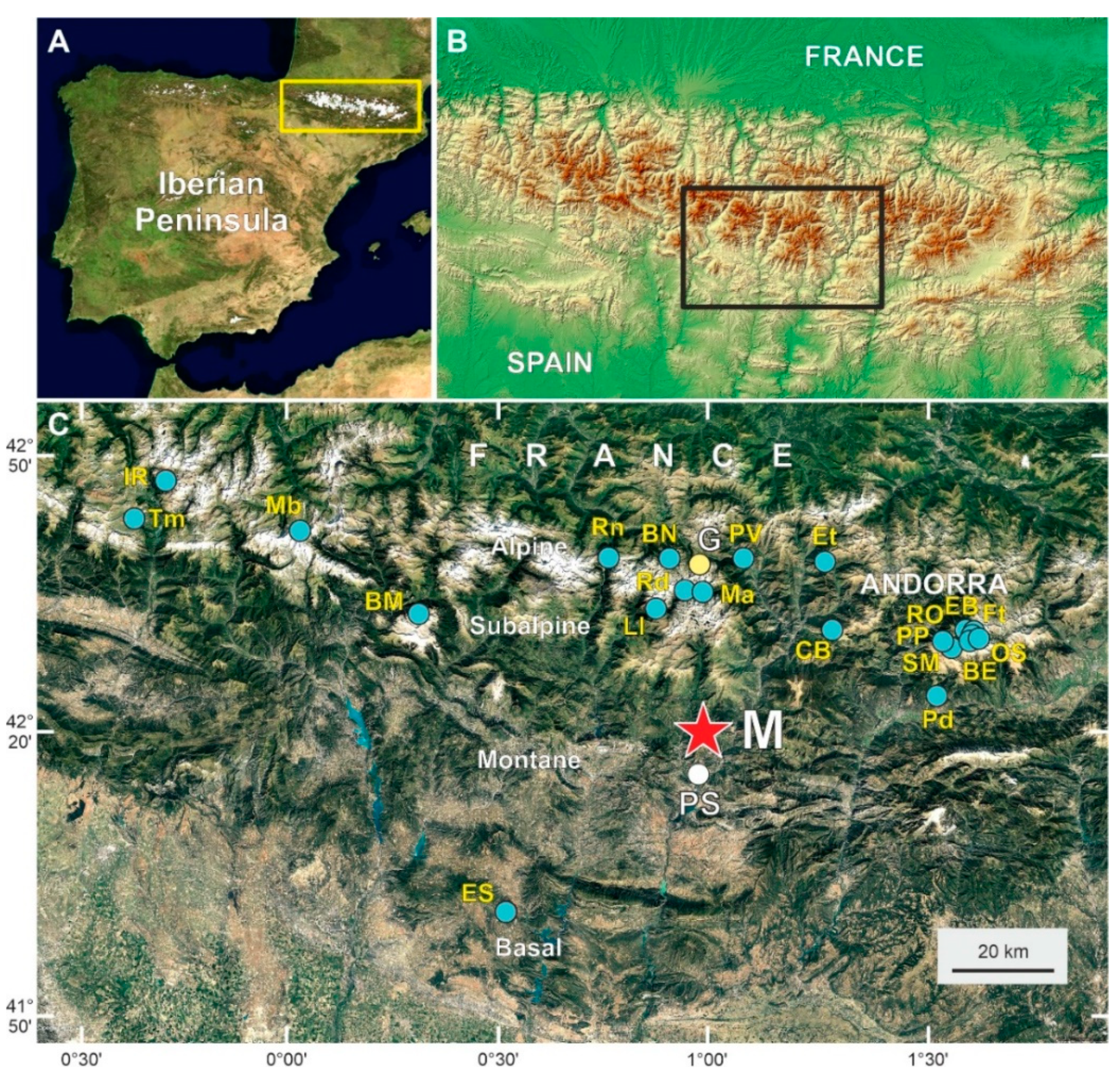
Lake Montcortès (42°19′50″ N–0°59′41″ E; 1027 m elevation) (Figure 1) is of karstic origin and is situated in the lowermost part of the montane belt (1000–1600 m), close to the transition with the lower (<1000 m) submontane Mediterranean belt. The closest weather station (La Pobla de Segur) is located approximately 9 km south at a 508 m elevation (Figure 1). There, the annual average temperature is 13.7 °C, with minima (3.2–3.5 °C) in January and December and maxima (23.9–24.3 °C) in July and August. Using the regional adiabatic lapse rate of −0.6 °C/100 m [50], Lake Montcortès would be approximately 3 °C colder on average. The total annual precipitation is 581 mm and exhibits a bimodal pattern, with maxima in spring (April–May: 66.1–66.4 mm) and autumn (October: 59.3 mm) and minima in winter (February: 19.4 mm) (Figure 2).
2.2. Regional Vegetation
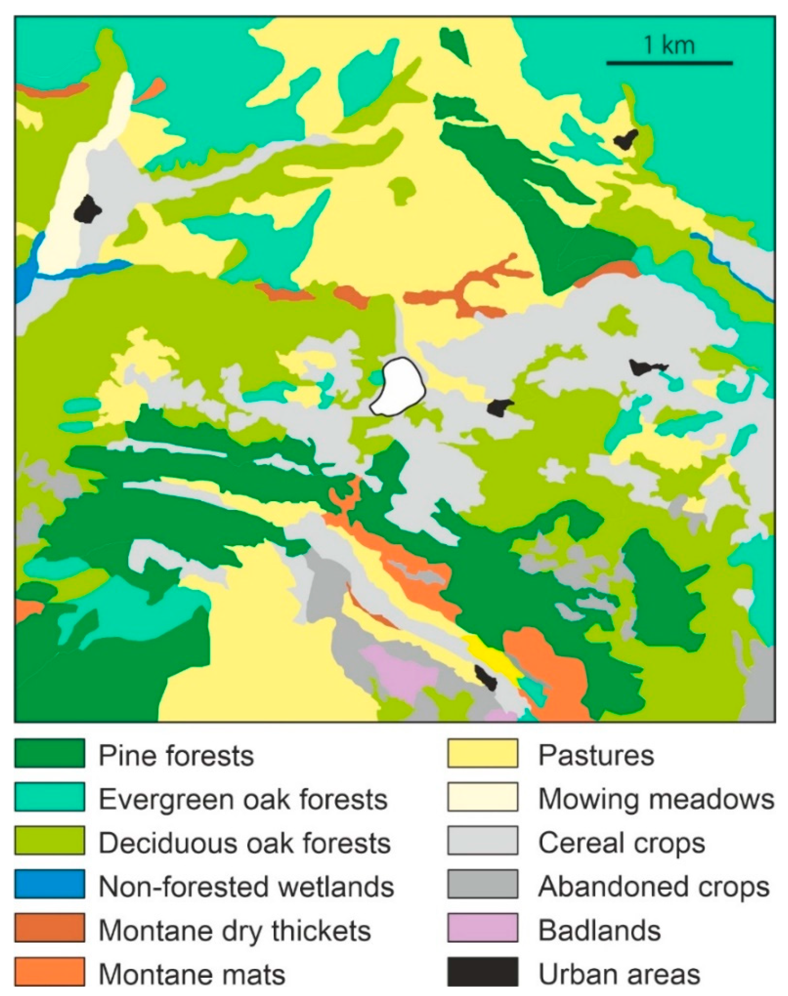
Four major forest formations occur around the lake catchment, reflecting its lowland/montane boundary conditions: (1) Mediterranean sclerophyllous forests of Quercus rotundifolia, (2) submontane deciduous oak forests dominated by Quercus pubescens and Q. subpyrenaica, (3) conifer forests of Pinus nigra (usually resulting from secondary replacement of the deciduous oak forests), and (4) higher-elevation montane forests of Pinus sylvestris, possibly including natural and planted forest stands [51]. The forests are arranged in a mosaic pattern, intermingled with other nonforested vegetation types (Figure 3). The first two forest communities are dominant around the lake. The evergreen Q. rotundifolia communities have a well-developed understory with several shrubs (Q. coccifera, Rhamnus spp., Prunus spinosa, Buxus sempervirens and Lonicera japonica) and an herbaceous stratum with nemoral (shade-adapted) species, such as Rubia peregrina, Teucrium chamaedris, Asparagus acutifolius, and Brachypodium retusum. The Q. pubescens-Q. subpyrenaica deciduous forests include a variety of other trees in the arboreal stratum, notably Pinus sylvestris, Fagus sylvatica, Tilia cordata, and some Acer species. The understory is dominated by Buxus sempervirens, Coronilla emerus, Amelanchier ovalis, Colutea arborescens, Cytisophilum sessilifolium, and Viburnum lantana. In the herbaceous stratum, the most common species are Primula veris, Hepatica nobilis, Brachypodium phoenicoides, and Campanula persicifolia [52].
There are two main types of shrublands: one dominated by Amelanchier ovalis, Buxus sempervirens, and Rhamnus saxatilis and another dominated by Arctostaphilos uva-ursi with Buxus sempervirens. Herbaceous communities primarily consist of meadows and pastures of Aphyllanthes monspelliensis and Arrhenaterum elatius, herbaceous cereal crops (Hordeum sp., Avena sativa, Triticum sp., Secale cereale) and some forage plants (Medicago sativa), with several weeds (Lolium rigidum, Papaver rhoeas, Polygonum aviculare, Bromus sp.). Abandoned croplands colonized by shrubs and ruderal species and badlands devoid of vegetation or with scattered shrubs and herbs from other communities also occur in some areas [51,52]. The lake is surrounded by a fringe of semiaquatic littoral vegetation dominated by Phragmites australis, Cladium mariscus, and Typha dominguensis. Beyond this fringe, on wet or inundated soils, the hygrophilous vegetation is dominated by Eleocharis palustris, Scirpus lacustris, and several species of Carex. Communities of temporarily flooded areas are dominated by Juncus bufonius and Cyperus fuscus [51].
The landscape of the Lake Montcortès catchment was anthropized in the Iron Age (770 BCE) after the removal of the Tilia-Corylus gallery forests that surrounded the lake and continued during Roman and Medieval times in the form of recurrent burning, grazing, cultivation, silviculture, and hemp retting [38]. During the last 3000 years (since the Late Bronze Age), regional forests have been dominated by Pinus and Quercus (deciduous and evergreen), as occurs today. Before the Modern Age, which is the target of this study, these forests underwent three major clearance events, during the Iron Age (~300 BCE), the Roman Period (~300 CE), and the Middle Ages (~1000 CE) [37]. Detailed reconstructions of the main paleovegetation trends are available for the Middle Ages [30] and the Modern Age [39].
3. Material and Methods
3.1. Raw Data
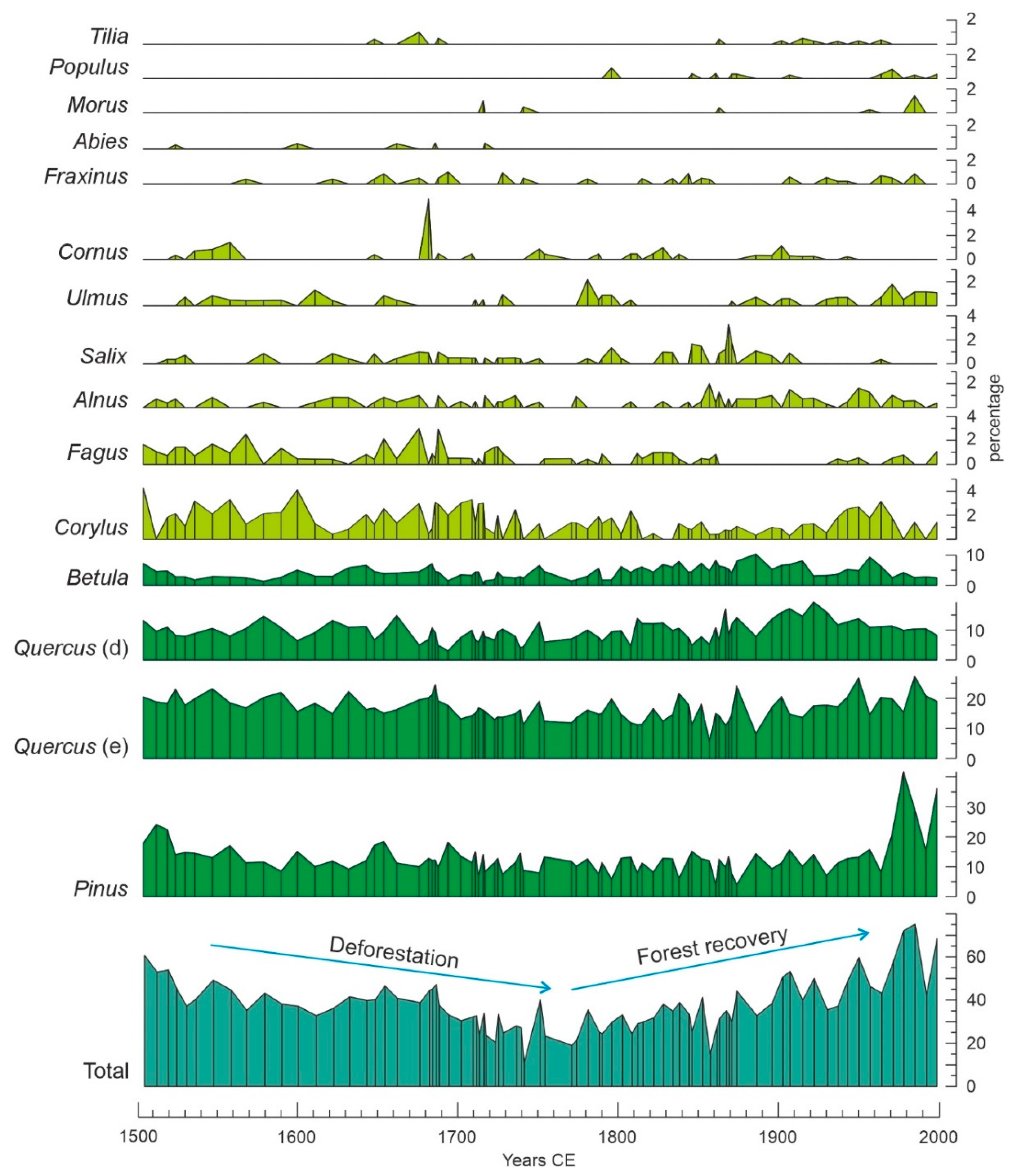
Raw pollen data for this study were taken from our own database after a former palynological analysis of Lake Montcortès sediment core MONT-0713-G05 covering the period 1423–2013 CE at subdecadal resolution (~6 yr/sampling interval, in average) [39]. A total of 96 samples were included in this database. Pollen percentages were recalculated after excluding hemp (Cannabis) from the pollen sum because there is strong evidence that hemp retting, rather than local cultivation of this plant, was the main source of Cannabis pollen during the Modern Age, which significantly distorts the percentage diagram and causes an artifact in the forest pollen curve [37]. The modified diagram of forest-pollen taxa is shown in Figure 4. Importantly, Quercus species cannot be identified by pollen due to their homogeneous morphology. However, it is possible to differentiate between deciduous and evergreen species groups, which in our case is useful because of the occurrence of two forest types dominated by deciduous (Q. pubescens and Q. subpyrenaica) and evergreen (Q. rotundifolia) species [51]. Another evergreen Quercus species present in the region is Q. coccifera, which occurs in the Q. rotundifolia forests and, hence, is morphologically consistent with the evergreen Quercus forest group.
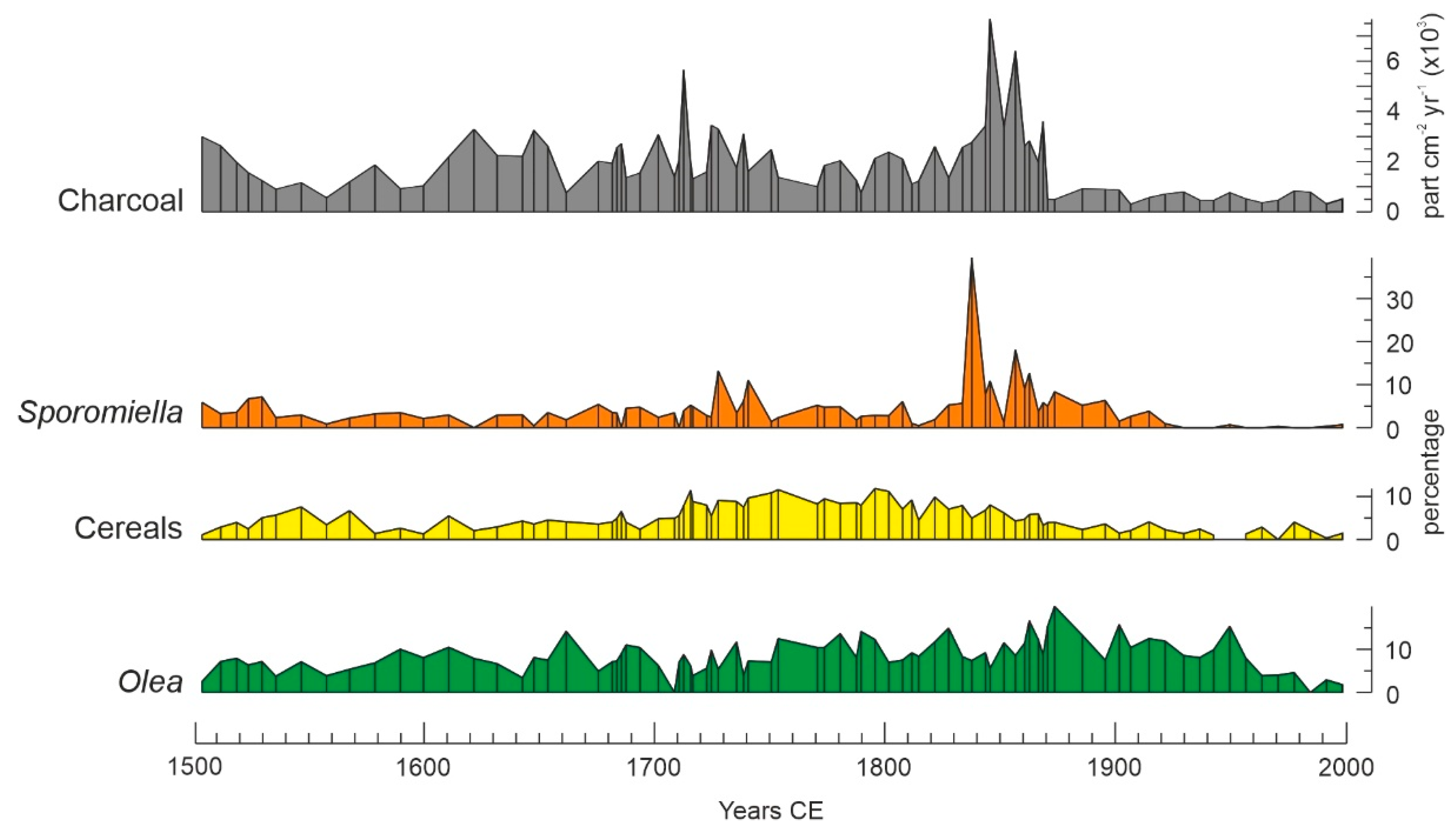
Proxies for human activities were cultivated trees (Olea) and herbs (cereals), the coprophilous fungus Sprormiella and charcoal (Figure 5). Only direct indicators of human presence have been considered. Olea is commonly cultivated in the lowlands just below Montcortès, and its pollen is well represented in the sediments of the lake [49]. Cereals (Secale, Triticum, and others) have also been common crops around the lake since historical times [37]. Sporormiella is a coprophilous fungus that lives in the feces of domestic animals and is thus a direct indicator of grazing [42]. Charcoal influx is the most commonly used proxy for fire intensity and has been recorded in the sediments of Lake Montcortès since the anthropization of the regional landscape [37,38]. Other cultivated trees (Castanea, Juglans) and herbs (Hedysarum) were not used due to their scarce and sporadic presence in the pollen record of the last few centuries [39]. Other pollen types related to human activities, such as weeds and ruderal plants (e.g., Artemisia, Plantago, Chenopodium, Rumex), have not been used in this analysis because they may occur naturally in the region, and their species cannot be reliably separated by pollen morphology. Therefore, it is difficult to disentangle the natural and anthropogenic contributions of these genera to the Montcortès sediments [41].
Two tree-ring-based paleotemperature reconstructions of the warmest season (summer) were used (Figure 6). One reconstructed the mean regional May–September paleotemperature and was obtained after the analysis of 22 site chronologies covering the whole Pyrenean range, from 1000 to 2500 m elevation, encompassing the period 1260–2005 CE [43]. The other paleotemperature reconstruction was obtained from a study performed in the catchment of Lake Gerber, a high-mountain lake situated ~30 km north of Lake Montcortès, at ~2170 m elevation (Figure 1). This record refers to the May–June and August–September average temperatures and covers the period 1186–2014 CE [44]. The same study was the source of the dataset for the intensity of the Mediterranean summer (July–August) drought. The reconstruction of autumn (September–November) precipitation—when the second peak of maximum annual precipitation is recorded (Figure 2)—was also taken from our own database and was generated by a study of varve thickness, as a precipitation proxy, on Lake Montcortès sediments [46]. A high-resolution (annual) study of extreme rainfall events is also available for Lake Montcortès sediments, based on detrital layers and turbiditic intervals, for the last 7 centuries [45]. However, the unsuitability of turbidites for pollen analysis [39] hinders the possibility of reliable statistical comparisons. All these time series, including those used in pollen analyses, were rescaled to the period 1504–2002 (498 years), which is the time period where they all overlap. This includes 80 of the 96 samples available in the palynological database [39].
Quantitative comparisons between paleoclimatic and palynological records required prior data standardization, as the first are of annual resolution while the second include several years in each sample. The abovementioned millimetric scale of varve thickness [53] complicates the collection of palynological samples of annual resolution, as a minimum of 1 cm3 of sediment is required for this type of analysis. To obtain this amount of material, core MONT-0713-G05 was sampled continuously at 5 mm intervals, avoiding turbidites [39]. As a result, palynological samples represented a variable number of years, from 1 to 17 (~6 on average). Statistical comparisons were performed between the results of palynological samples, whose data are considered to be averages of the years represented by each sample, and the calculated average of paleoclimatic data for the years represented in each palynological sample. For example, the sample corresponding to 1802 CE contains 6 varves/years (1797–1802 CE), and its palynological results were compared with the average of the estimated climatic parameters for these 6 years.
3.2. Statistical Methods
The first step was the analysis of individual tree pollen types with respect to external (climatic and anthropogenic) variables. Paleoecological evidence has been instrumental in showing that species respond individually to environmental changes according to their idiosyncratic features, and this determines changes in forest composition over time [54]. In addition, human pressure on forest trees is usually selective, as some species are preferred for exploitation and/or deforestation targets. Therefore, individual relationships among forest-tree species and external forcings could be highly informative. These relationships were addressed using nonlinear Gaussian response models along environmental gradients [55,56] (Figure 7).
Critical elements in the differential species responses to climatic shifts are temporal response lags, which vary across species and may be especially relevant in organisms with long life cycles, such as forest trees [33]. Here, the response lags were estimated by stepwise correlation after sequential 1-sample offsets between climatic and taxon series. Owing to the abovementioned subdecadal resolution of pollen samples, the resulting sample lags encompassed ~6 yr on average (Section 3.1). The process was repeated until a maximum lag of roughly a century, which has been considered enough to detect eventual response lags in 500 yr-long time series like those studied here. In the case of anthropogenic proxies, the responses are considered to be immediate (at subdecadal average resolution), as activities such as cultivation, grazing, tree felling, and burning instantaneously affect the involved ecosystems. In spite of this, some of these activities would have different scales of spatial impact. For example, some types of cultivation can be considered a factor of more local significance, whereas burning would be of more regional scope.
In a second step, cluster analysis was used to define the assemblages of forest-tree pollen in sedimentary samples. The Pearson coefficient was used as the measure of similarity, and the unweighted pair group average (UPGMA) approach was the selected clustering approach [57,58]. The assemblages obtained were used to calculate the rate of change, expressed as the standardized Euclidean distance (SED) between adjacent pairs of samples [59]. The combination of these analyses yielded a general overview of the forest types involved in regional forest succession and the amount of total change in these forest types over time.
The third step was aimed at reconstructing the regional forest succession itself using principal component analysis (PCA), the usefulness of which has been demonstrated for ecosystems under climatic and anthropogenic forcing, by defining attraction domains and following the sample chronology to define the successional trajectories around these domains [60]. In this case, raw data (tree-pollen percentages only) were centered due to the homogeneity of the data matrix [61]. The number of significant principal components was determined according to Kaiser’s rule, which establishes that the minimum significant eigenvalue should be the average of all eigenvalues [62].
In a fourth step, a synthetic analysis of successional trends and the influencing external variables was addressed by redundancy analysis (RDA), using tree taxa in the variable matrix and climatic/anthropogenic factors in the environmental matrix [62]. RDA was preferred over canonical correspondence analysis (CCA) due to the results of previous statistical analysis, which showed near-linear responses of major taxa to external drivers (Figure 7). To optimize RDA outputs and minimize noise, input variables were selected according to the results of previous statistical analyses. Indeed, only forest taxa with significant responses in the individual analysis and with high variable loadings in the PCA were considered. The possibility of multicollinearity among environmental variables was addressed using the values of inflation factors as a criterion [63].
All these statistical analyses and graphical display of the results were carried out with MVSP 3.22 (www.kovcomp.co.uk/mvsp/ accessed on 14 April 2022) [64,65], Past 4.09 (https://www.nhm.uio.no/english/research/infrastructure/past/ accessed on 14 April 2022) [66,67] and Psimpoll 4.27 (https://chrono.qub.ac.uk/psimpoll/psimpoll.html/ accessed on 14 April 2022) [68]. The graphics were edited to improve homogeneity and visualization.
4. Results
4.1. Individual Responses of Tree Taxa to External Drivers
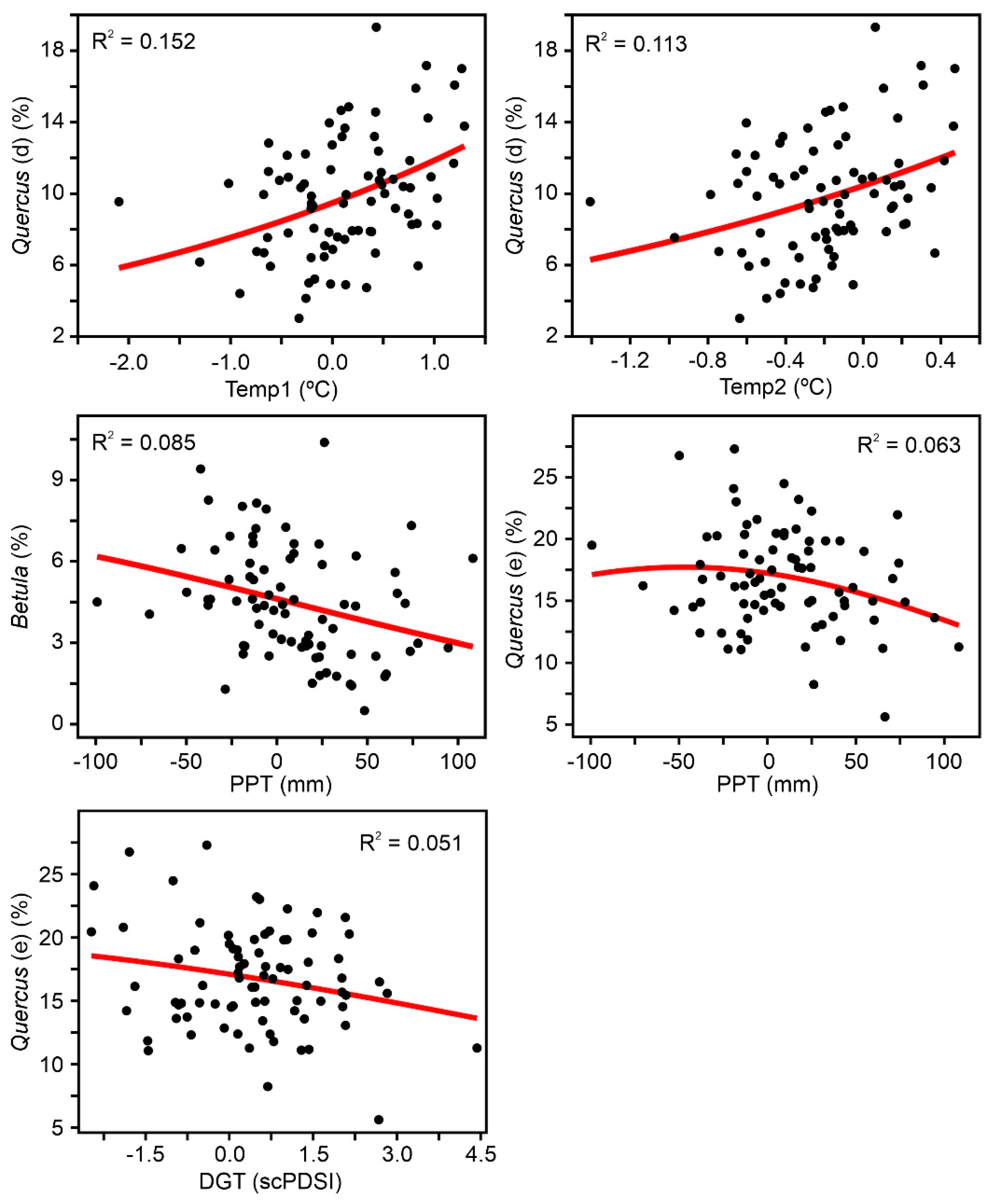
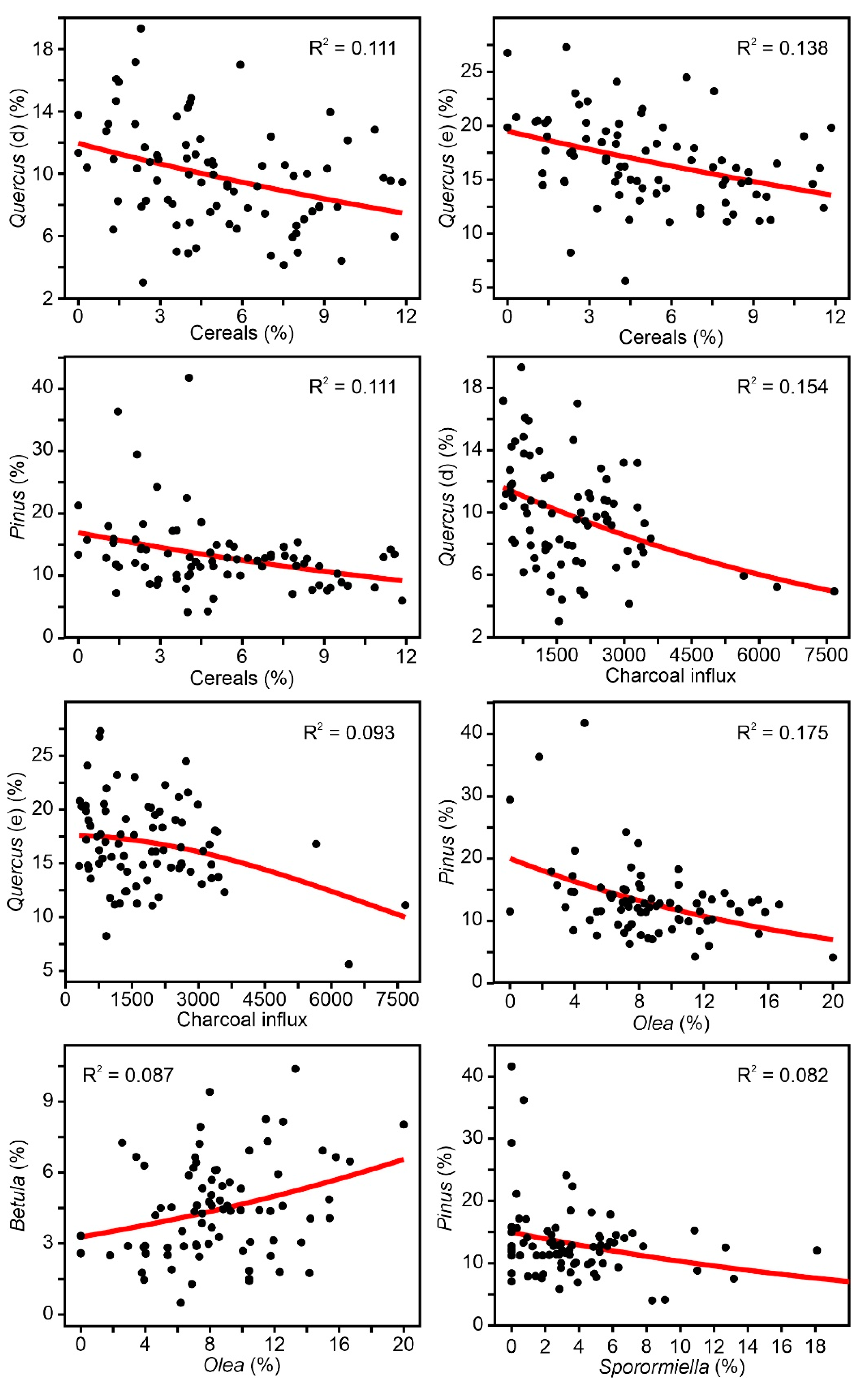
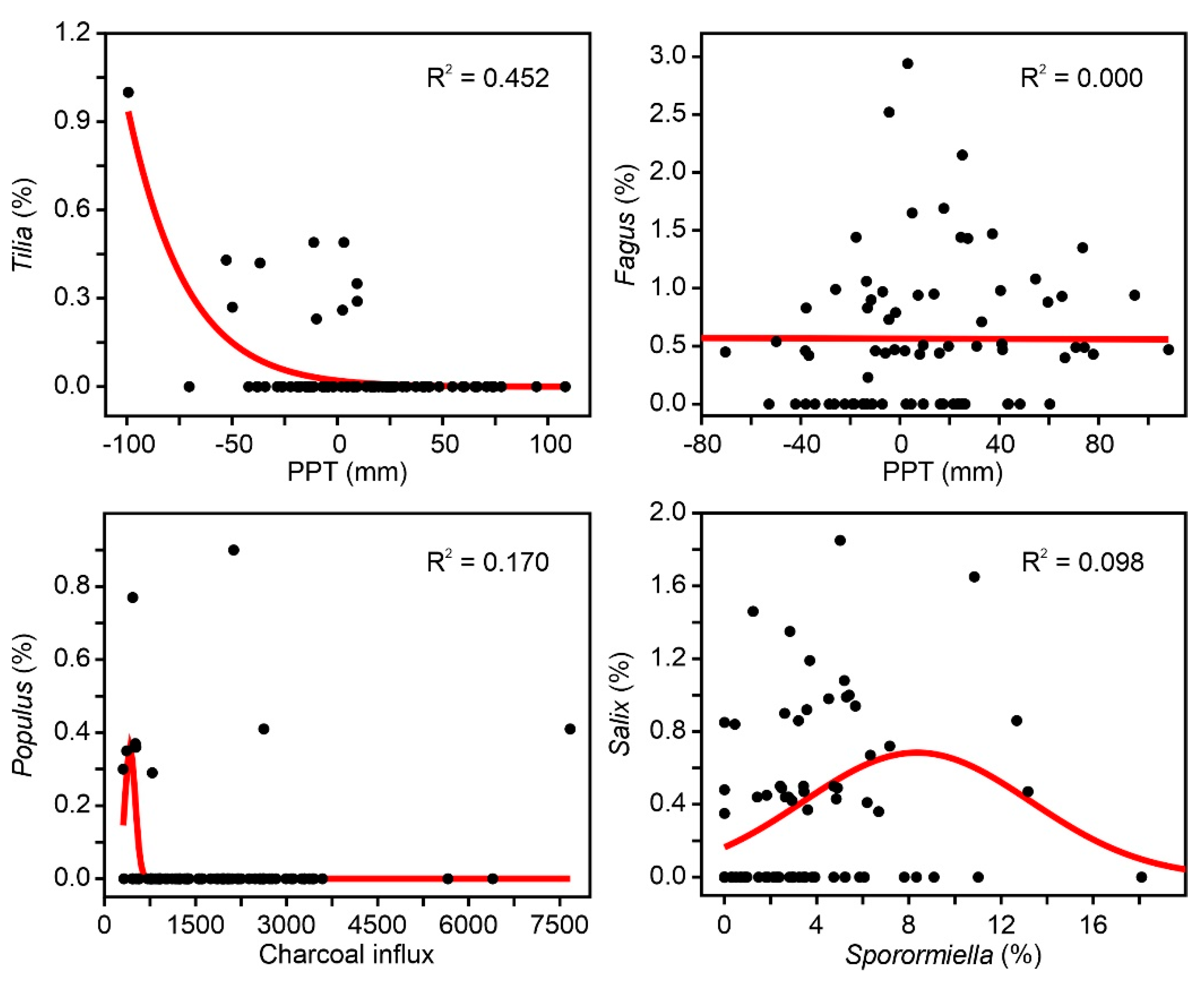
The results of the Gaussian response analysis are shown in Figure 8, Figure 9 and Figure 10. Figure 8 shows the forest taxa with significant responses to climatic parameters, and Figure 9 displays the taxa with significant responses to anthropogenic indicators. The critical significant correlation coefficient (n = 80; p < 0.05) is r = 0.217 (R2 = 0.047). The most illustrative examples of nonsignificant or misleading relationships are shown in Figure 10. The most frequent case is illustrated by Fagus-PPT, which is characterized by nonsignificant relationships represented by flat trends (R2 = 0.000). In other cases, higher R2 values were influenced by the occurrence of many zero values, which is considered to be a statistical artifact leading to false response models [69,70]. Figure 10 shows a selection of different unwarranted response models due to excess zero values, a situation that affected almost all minor forest components (Figure 4). As a result, only the four dominant forest taxa (deciduous and evergreen Quercus, Betula, and Pinus) were useful for this response analysis (Figure 8 and Figure 9).
As all significant taxon–environment relationships suggested nearly linear or exponential trends (Figure 8 and Figure 9), the response analysis was completed with linear and exponential regression analyses. Table 2 shows the correlation coefficients under linear and exponential models. The best fit was linear in 6 cases and exponential in 9 cases. Among the linear models, only two showed negative correlations (Betula-PPT and Quercus (e)-DGT), whereas all exponential models showed negative correlations. Interestingly, linear and exponential correlation values showed small differences that did not affect significance patterns. Two new significant correlations emerged from this analysis that were not detected in the Gaussian analysis: Quercus (d) and Quercus (e) with Sporormiella, both of which were exponential and negative.
To summarize the results of Table 2, it can be said that the most influential climatic parameters were summer temperature (Temp1 and Temp2) and autumn precipitation (PPT), whereas tree/herb cultivation, grazing, and fire incidence were the most relevant anthropogenic drivers at the individual taxonomic level. All of the dominant forest taxa showed significant negative correlations with most anthropogenic factors except Betula, which was positively correlated only with tree cultivation. Deciduous Quercus was the only forest element correlated (positively) with summer temperature, while Betula and evergreen Quercus were associated with autumn precipitation. Pinus was not significantly related to any climatic parameters. The linear/exponential nature of the significant relationships suggests that the dataset utilized covers only part of the environmental range of the involved taxa (Figure 7). This may indicate that the range of variation in the selected environmental parameters during the last 500 years has occurred at suboptimal values for the dominant forest taxa.
The above individual analyses assume immediate (at subdecadal average resolution) responses of forest trees to external variables, as they compare pollen abundance and paleoclimatic estimates from the same sample intervals. The possibility of response lags between climatic shifts and forest trees has been addressed, and the results obtained are explained below (Figure 11). In the case of deciduous Quercus, positive correlations with summer temperature (Table 2) were maintained for lags of ~20 and ~40 years, whereas autumn precipitation and summer drought intensity, which were nonsignificant in previous analyses, showed significant response lags of ~40 years. Therefore, a 40 yr response lag was present for all climatic parameters, which suggests that deciduous Quercus has been sensitive to all these climatic drivers and has had two types of responses, one that was immediate (at subdecadal average resolution) and another that was delayed for 40 years.
Evergreen Quercus was different, as it showed a response lag to summer temperature of ~15 years, which was maintained until an ~80 yr lag, with intermediate peaks at ~50 and ~60 yr. In contrast, the response to autumn precipitation and summer drought intensity was immediate (Table 2) and only showed a significant lag of ~20 yr in response to precipitation. Betula, which only responded immediately to precipitation (Table 2), showed an ~15 yr response lag to summer temperature and autumn precipitation and a 50–60 yr response lag to summer drought. As in the case of deciduous Quercus, evergreen Quercus and Betula showed two types of responses (immediate and ~15–20 yr delayed) for the same climatic factor (autumn precipitation). Finally, Pinus, which did not respond immediately to any climatic drivers (Table 2), showed several response lags for summer temperature (~30 yr, ~50 yr, ~70 yr, ~100 yr) and only one ~100 yr response lag to summer drought intensity. In summary, all major forest taxa responded to most climatic drivers, showing different response lags characteristic of each taxon.
4.2. Forest Assemblages and Rate-of-Change Analysis
Cluster analysis revealed three different forest assemblages: A1, dominated by deciduous Quercus; A2, dominated by evergreen Quercus; and A3, dominated by Pinus (Figure 12). These assemblages coincide with the forest types characteristic of the Montcortès region (Section 2: study site), which indicates that these forests have also been dominant during the last 500 yr. Figure 13 shows that forest succession has progressed by variations in the abundance of individual taxa within each forest type, rather than by community turnover. The most significant successional fluctuations have been identified by rate-of-change (ROC) analysis, which shows a period of more intense shifts between ~1680 CE and ~1870 CE (Figure 13). This phase coincides with maximum deforestation (Figure 4) and the intensification of human activities around the basin, as indicated by increases in cereal cultivation, grazing intensity (Sporormiella), and fire incidence (charcoal) (Figure 5). The onset of this phase is also coeval with the minimum estimated values of autumn precipitation, while the end coincides with an increase in summer temperatures (Figure 6).
4.3. Successional Trends
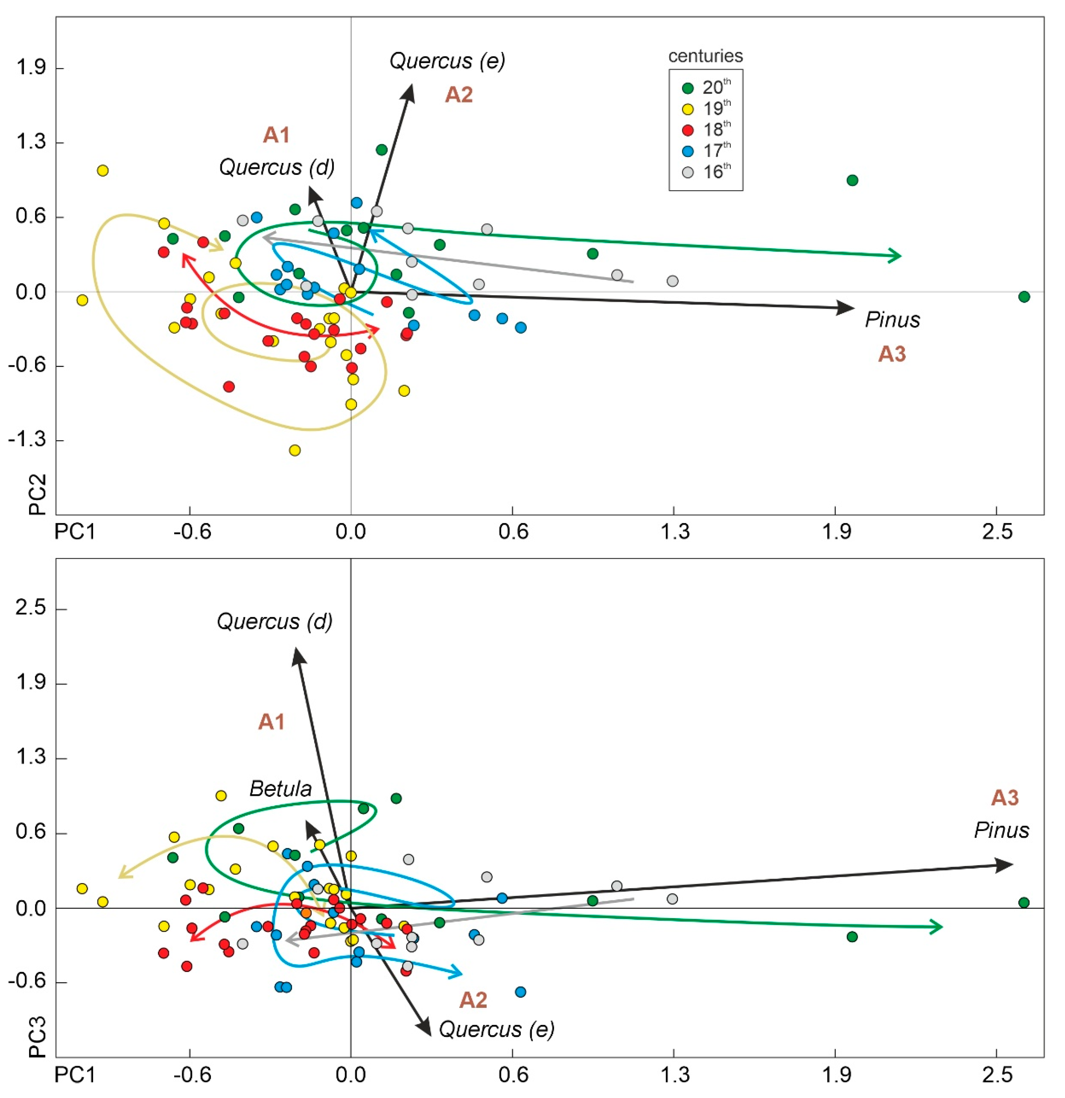
In the PCA performed here, the first three components (PC1 to PC3) were significant (>91% of the total variance) and were statistically associated with Pinus (PC1), evergreen Quercus (PC2), and deciduous Quercus (PC3) (Table 3), respectively, coinciding with the assemblages defined in the cluster analysis (Figure 13). Using the sample scores and their corresponding ages, the regional successional trends could be reconstructed in relation to the attraction domains represented by the dominant trees and the assemblages they represent. Successional trends were subdivided into arbitrary segments represented by the 16th to 20th centuries to facilitate description and visualization.
The succession began around the attraction domain A3 (dominated by Pinus) and showed a nearly linear trend toward the A1 (dominated by evergreen Quercus and Betula) and A2 (dominated by deciduous Quercus) domains during the 16th century (Figure 14). In the 17th century, successional trends adopted an oscillating trajectory, mainly around domains A1 and A2. The situation was similar in the 18th century, but this time, oscillating trends showed some departure from the A1/A2 domains, at least on one of the shifting sides. This deviation increased during the 19th century, when a spiral-like trajectory developed that returned the succession to domain A2. During the 20th century, the trend started in this attraction domain and, after a nearly circular trajectory between A1 and A2, followed a maintained and straightforward trend toward A3, near the attraction domain where the whole successional process began. In summary, regional forest succession started in A3 and, after defining oscillating/spiral/circular trajectories around A1 and A2, returned to A3. Notably, successional trends proceeded around attraction domains A1 to A3 during the 16th, 17th, and 20th centuries, when rate-of-change values were minimal (Figure 13), and showed some departures from these domains during the 18th and 19th centuries, when rate-of-change values were high and some anthropogenic proxies (notably cereals, Sporormiella, and charcoal) reached their maxima (Figure 5).
4.4. Synthetic Successional-Environmental Analysis
As discussed in the methods (Section 3.2), RDA was the preferred synthetic gradient analysis because CCA assumes unimodal responses of species to environmental drivers and, in the case analyzed here, these responses were nearly linear (Figure 8 and Figure 9). The selected taxa for the RDA were evergreen Quercus, deciduous Quercus, Pinus, and Betula due to their significant responses in the former Gaussian analysis and highest variable loadings in the PCA (Table 3). A first run revealed collinearity between the environmental variables Temp1 and Temp2 (inflation factors >5). Indeed, these variables were highly correlated (r = 0.857; p < 0.001), and one of them (Temp2) was removed from the analysis to avoid potential distortions [61]. The final RDA run yielded two significant axes, accounting for 25.38% of the total variance, with highly significant (p < 0.001) taxon-environment correlations (0.624 for axis 1 and 0.498 for axis 2). The R2 (0.277) of the overall test was also significant at p < 0.001.
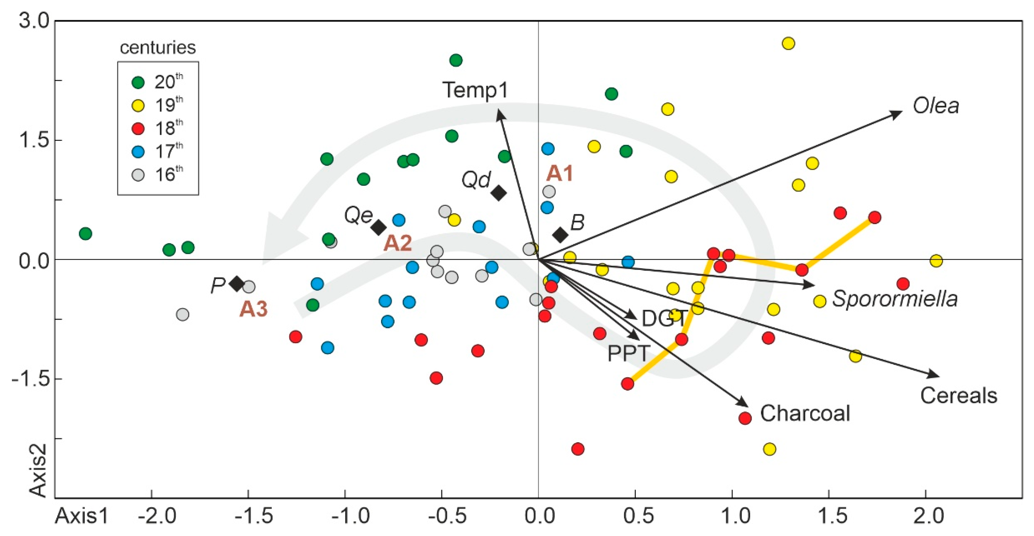
The scores of samples, taxa, and explanatory variables with respect to the two significant RDA axes are shown in Figure 15, where a clear left-right ordination can be seen. Samples belonging to the 16th, 17th, and 20th centuries are situated mostly in the left hemisphere, whereas the right side contains most samples from the 18th and 19th centuries. The same pattern was observed in the ROC analysis (Figure 13). In the RDA graphical framework, the global successional trends define a loop beginning and ending near Pinus, the dominant taxon of A3. This is consistent with successional trends defined in the PCA, which showed that succession started in the A3 domain in the 16th century; progressed to the A2 and A1 domains, where it remained during the 17th to 19th centuries; and finally returned to the A3 domain following the reverse pathway (A1 and A2) in the 20th century. The positions of major forest taxa in the RDA plot (Figure 15) also agree with this temporal sequence, as successional trends began close to Pinus (the dominant taxon of A3), progressed through deciduous Quercus and Betula (A1), and turned back toward Pinus after passing by evergreen Quercus (A2).
All explanatory (environmental) variables except Temp1 are situated on the right side, together with samples corresponding to the 18th and 19th centuries (Figure 15). The most influential variables (longer vectors) were the anthropogenic drivers, which suggests that succession was mainly controlled by these factors during the 18th and 19th centuries. The order of these vectors in the scatter plot suggests that the sequence of anthropogenic actions would have been burning, cereal cultivation, grazing, and lowland olive cultivation. The phase of maximum deforestation (1740–1770 CE) coincided with the first three of these anthropogenic drivers. Regarding climatic drivers, PPT and DGT seem to have been important in the transition from the left to the right side (17th–18th centuries), whereas Temp1 was likely more relevant in the final successional stage, during the 20th century, when forest recovery progressed in the sequence A1-A2-A3. Notably, whereas Temp1 is far from any anthropogenic variable, PPT and DGT are strongly associated with charcoal, which may suggest some type of interaction among these factors.
5. Discussion and Conclusions
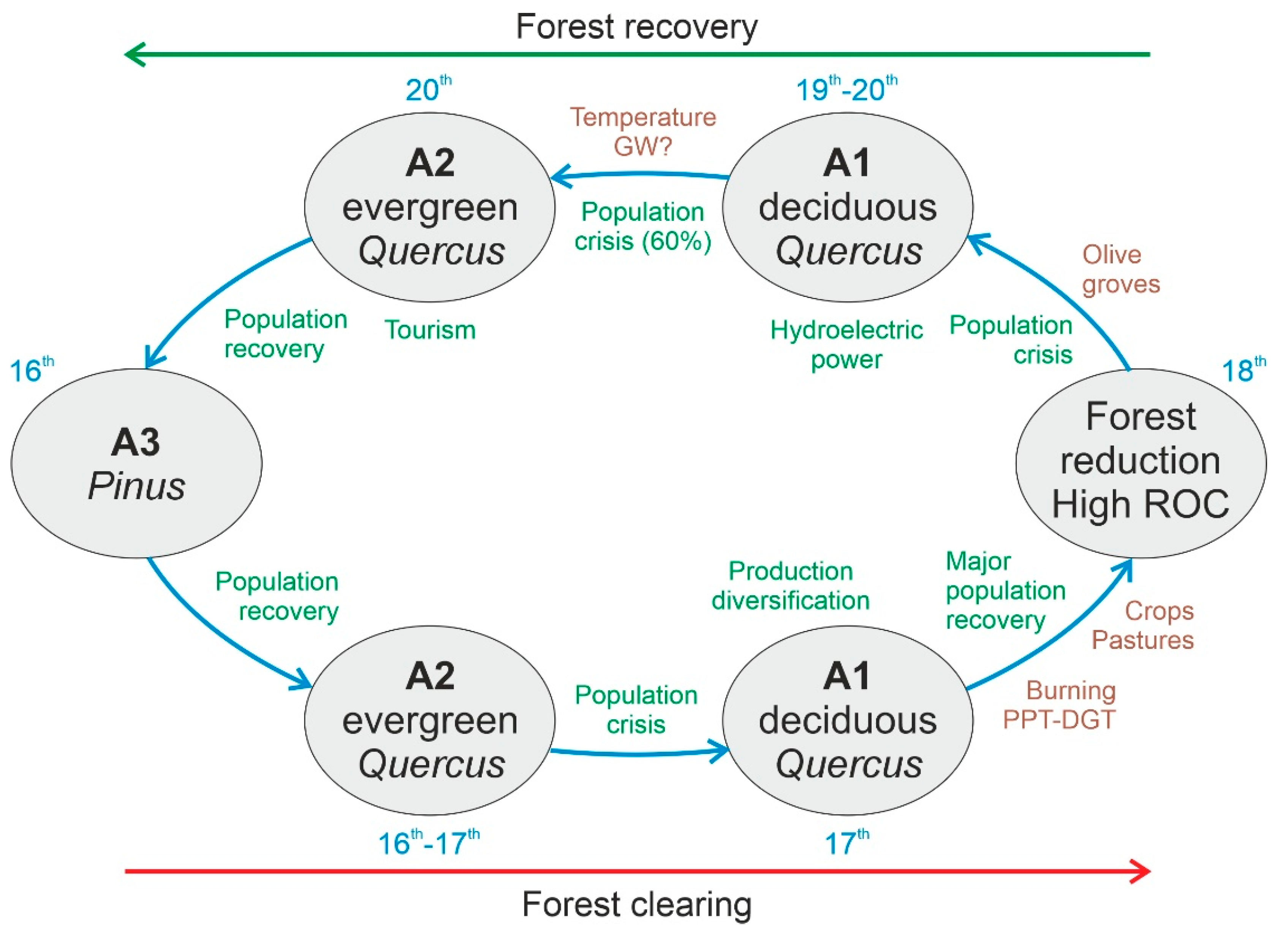
Regional forest succession around Lake Montcortès over the last 500 years can be represented by four main stages defining a loop, which started and ended with the prevalence of forest assemblage A3, dominated by Pinus (Figure 16). Forest assemblages A1, A2, and A3 were present during the whole period of study, but their cover and spatial patterns varied under the influence of climatic and anthropogenic factors. The stages represented in Figure 16 have been named according to the prevalent forest assemblages. Maximum forest reduction affected the dominant taxa of all assemblages (Figure 4 and Figure 13). The succession began in A3 (early 16th century) and moved to A2 and A1 during the 16th and 17th centuries. No clear climatic or anthropogenic drivers are associated with this trend (Figure 16) but the occurrence of the Maunder Minimum between 1645 and 1715 could have been involved, as it coincided with a conspicuous precipitation decline [46] (Figure 6). At the beginning of the 18th century, forest burning initiated trends toward forest reduction, involving all forest assemblages (A1 to A3), which alternated at high rates of change (Figure 13). Fires would have been favored by the intensification of summer droughts due to the enhanced flammability of vegetation. Drier summers were followed by wetter autumns (r = 0.382; p < 0.001), but this would have had little effect on forests, as autumn is not a growing season for trees. The deforested terrains around Lake Montcortès were used for cereal cultivation and pastures. Maximum deforestation occurred in the mid-18th century and was followed by a trend toward forest recovery, coinciding with the maximum development of olive groves in the adjacent lowlands. Forest recovery followed the reverse trend of forest clearing (A1 and A2) and was likely favored by rising summer temperatures, which would have fostered tree growth. In the late 20th century, the succession ended with the recovery of the pine-dominated assemblage (A3). The increase in summer temperature could be linked to global warming (GW) initiated in the mid-19th century], and the increase in Pinus could have also been favored by human forest management.
The existence of detailed and well-documented historical records for the Pallars region [71,72], to which Lake Montcortès belongs, facilitates comparison between our paleoenvironmental and paleoecological results and the main cultural developments. In the Pallars, the Modern Age began in 1488 CE [73], just after the end of the Medieval crisis (1350–1487 CE), when the region was significantly depopulated due to the coincidence of wars, epidemics (Black Death), climatic deterioration (Little Ice Age), and the self-induced collapse of the feudal system [74]. A rapid but short-lived population recovery was initiated in the 16th century, followed by a second crisis in the 17th century and an additional larger and more stable population recovery [75]. These population trends are consistent with the stages of forest succession, as the progress from A3 to A2 and A1 occurred in a phase of lower human impact (16th to mid-17th centuries), whereas the acceleration of forest clearing (mid-17th to mid-18th centuries) coincided with an increase in anthropogenic pressure culminating in 1750 CE, when deforestation was maximal (Figure 16). The population crisis of the 17th century also influenced the type of land use, and a shift toward productive diversification occurred, including the exploitation of forests for wood and the transformation of crop fields into pastures [75], which is also consistent with our successional trends (Figure 15 and Figure 16). Forests were not burnt or exploited extensively, as occurred in the Middle Ages [74], but were submitted to controlled wood extraction by particular or communal owners, especially from the 18th century onward [75]. This led to lower deforestation levels compared to those in Medieval times [30] and favored regional forest recovery beginning in the mid-18th century [37] (Figure 16).
The period between the late 18th and late 19th centuries was characterized by the physical isolation of the Pallars region and the predominance of a subsistence economy. However, the failure of this type of self-sufficient economy led to another population crisis, characterized by emigration to large cities beyond the Pallars region and foreign countries [75]. A new economic model emerged in the early 20th century with the development of hydroelectric power and the associated industrialization and communication infrastructures, which fostered a population increase. However, in the 1960s, the full industrialization of large cities far from the Pallars region promoted massive emigration from rural to urban areas, which caused the loss of approximately 60% of the Pallars population. The late 20th century witnessed economic recovery due to the development of tourism for urban consumers, and traditional economic activities, such as farming and forestry, have been progressively lost [75]. In summary, the population crises of the late 19th and 20th centuries, along with the progressive abandonment of traditional farming activities in favor of hydroelectricity and tourism industries, favored forest regeneration (Figure 16). Considering the coincidence of these local cultural trends with ongoing GW, the process of forest recovery observed since the 19th century could also be the result of synergies between climatic and anthropogenic factors. It is also worth noting that some pine-dominated forests could have been planted in recent decades [51].
It should be noted that the analyses leading to the above conclusions have been performed by comparing taxa and environmental variables corresponding to the same sample interval, as we did in the case of individual taxon–environmental relationships. As we have seen, this contemporaneity did not represent a problem for anthropogenic drivers, as they generate immediate ecological responses, but the situation is different for climatic factors. Indeed, in the response lag analyses, we realized that some taxa responded immediately (at the subdecadal level) to climatic shifts, but others exhibited response lags of two or more decades. There were also taxa that showed both instantaneous and delayed response types to the same climatic parameter (Figure 11). Immediate responses could be generated by modifying pollen production and release to the air during the flowering season that, in the NE Iberian Peninsula, are known to be positively affected by temperature and insolation and negatively affected by precipitation [76]. Responses delayed for two or more decades are more attributable to long-term population dynamics and the resulting expansion or contraction of the geographical ranges of the involved species and the forest assemblages they dominate [77,78]. In the case of century-scale (>100 yr) delays, potential statistical artifacts should not be dismissed but more studies are needed for a sound assessment. Response lags can complicate the interpretation of statistical outputs in climatic terms, and in the present state of knowledge, the occurrence of response lags as potentially distorting factors cannot be dismissed. The inclusion of additional climatic variables known to affect tree taxa would also be desirable, but unfortunately, high-resolution paleoclimatic reconstructions of this type are still unavailable for the studied region. It would be also interesting to consider lower-frequency (decadal, centennial) climatic oscillations that could affect forest succession.
The results of the response lag analysis constitute a warning for studies aimed at detecting instantaneous relationships between climatic and ecological shifts. In our case, we have been able to establish some immediate ecological relationships with some climatic drivers showing significant correlations. However, the lack of significant Gaussian/linear/exponential responses to other variables does not necessarily mean that these climatic drivers did not affect forest succession, as the responses could be lagged for decades. This topic is a research target by itself and will be investigated in further analyses. A general conclusion that can be drawn from the present analysis is that both climatic and anthropogenic factors, along with interactions between them, have influenced forest succession. Therefore, the former inferences based on nonstatistical qualitative analysis that only human pressure has affected paleovegetation trends in the Montcortès region and climate has exerted an indirect influence by modulating human dynamics should be reconsidered.
6. Final Remarks
Unfortunately, it is not possible to compare our results with those of other studies at a regional level due to the absence of similar investigations. In contrast with most of the available palynological records from the central Iberian Pyrenees (Table 1), those used in this paper were obtained with an approach that is eminently ecological rather than environmental. Paleoenvironmental investigations aimed at reconstructing climatic and anthropogenic parameters from pollen proxies are not unusual, but they may foster circularity. Indeed, the response of forests to external drivers cannot be assessed if both environmental and forest trends are deduced from the same palynological proxies. Another relevant contribution of our analysis is that potential relationships between forest dynamics and external factors have been analyzed statistically using large datasets rather than inferred from a visual comparison of the corresponding trends. Additionally, our analyses were conducted at high temporal resolution (subdecadal), which is the most reliable approach for reconstructing ecological forest succession. Finally, we used high-resolution (annual) paleoclimatic estimates obtained from the same lake sediments or at nearby sites, including a temperature reconstruction representing the whole Pyrenean range. In summary, we consider that the fulfillment of at least these four conditions—(i) the independence between forest and environmental proxies, (ii) the development of high-resolution paleoecological records, (iii) the use of local or regional paleoclimatic reconstructions, and (iv) the application of suitable statistical methods—is fundamental to address this type of investigation. Neglecting these conditions may lead to questionable conclusions about the influence of climatic and anthropogenic drivers on forest dynamics and succession. This is a relevant observation, as predicting the responses of forests to present and future climatic/anthropogenic change is a serious conservation challenge that needs long-term ecological observations like those used in this work. Approaches failing to meet the abovementioned conditions will likely be unable to furnish the reliable long-term ecological background required to anticipate future successional trends and to feed predictive ecological models.
Author Contributions
Conceptualization, methodology, formal analysis, investigation, writing, V.R.; resources, review and editing, project administration, funding acquisition, T.V.-V. All authors have read and agreed to the published version of the manuscript.
Funding
Spanish Ministry of Economy and Competitiveness, projects CGL2012-3665 and CGL2017-85682-R.
Data Availability Statement
Present-day climatic data are publicly available at the Catalan Meteorological Service (https://www.meteo.cat/wpweb/climatologia/serveis-i-dades-climatiques/series-climatiques-historiques/, accessed on 20 February 2022). Raw data for Temp1 and drought intensity (DGT) reconstructions were provided by U. Büntgen. Raw data for Temp2 reconstruction were downloaded from the public NOAA’s National Centers for Environmental Information (https://www.ncei.noaa.gov/access/paleo-search/study/1003405, accessed on 20 February 2022). Data on autumn precipitation reconstruction (PPT) are from the own author’s database, and are in the process of being uploaded to public databases. Chronostratigraphic and palynological data are publicly accessible at Mendeley Data (data.mendeley.com/datasets/cdnjkyp4gz/1, accessed on 20 Februray 2022).
Acknowledgments
The authors are grateful to Ulf Büntgen for kindly providing raw data on temperature and drought reconstructions.
Conflicts of Interest
The authors declare no conflict of interest.
References
- Falk, D.A.; van Mantgem, P.J.; Keeley, J.E.; Gregg, R.N.; Guiterman, C.H.; Tepley, A.J.; Young, D.; Marshall, L.A. Mechanisms of forest resilience. For. Ecol. Manag. 2022, 512, 120129. [Google Scholar] [CrossRef]
- Trugman, A. Integrating plant physiology and community ecology across scales through a trait-based models to predict drought mortality. New Phytol. 2022, 234, 21–27. [Google Scholar] [CrossRef] [PubMed]
- Yi, C.; Hendrey, G.; Niu, S.; McDowell, N.; Allen, C.D. Tree mortality in a warming world: Causes, patterns, and implications. Environ. Res. Lett. 2022, 17, 030201. [Google Scholar] [CrossRef]
- Willis, K.J.; Bailey, R.M.; Bhagwat, S.A.; Birks, H.J.B. Biodiversity baselines, thresholds and resilience: Testing predictions and assumptions using palaeoecological data. Trends Ecol. Evol. 2010, 25, 583–591. [Google Scholar] [CrossRef]
- Willis, K.J.; Birks, H.J.B. What is natural? The need for a long-term perspective in biodiversity conservation. Science 2006, 314, 1261–1265. [Google Scholar] [CrossRef] [Green Version]
- Vegas-Vilarrúbia, T.; Rull, V.; Montoya, E.; Safont, E. Quaternary palaeoecology and nature conservation: A general review with emphasis on the Neotropics. Quat. Sci. Rev. 2011, 30, 2361–2388. [Google Scholar] [CrossRef]
- Rull, V.; Vegas-Vilarrúbia, T. What is long term in ecology? Trends Ecol. Evol. 2011, 26, 3–4. [Google Scholar] [CrossRef]
- Smol, J.P.; Last, W.L. (Eds.) Tracking Environmental Change Using Lake Sediments; Springer: Dordrecht, The Netherlands, 2002. [Google Scholar]
- Dubois, N.; Jacob, J. Molecular biomarkers of anthropogenic impacts in natural archives: A review. Front. Ecol. Evol. 2016, 4, 92. [Google Scholar] [CrossRef] [Green Version]
- Castaneda, I.S.; Schouten, S. A review of molecular organic proxies for examining modern and ancient lacustrine environments. Quat. Sci. Rev. 2011, 30, 2851–2891. [Google Scholar] [CrossRef]
- Leunda, M.; González-Sampériz, P.; Gil-Romera, G.; Aranbarri, J.; Moreno, A.; Oliva-Urcia, B.; Sevilla-Callejo, M.; Valero-Gracés, B. The Late-Glacial and Holocene Marboré Lake sequence (2612 m a.s.l., Central Pyrenees, Spain): Testing high altitude sites sensitivity to millennial scale vegetation and climate variability. Glob. Planet. Chang. 2017, 157, 214–231. [Google Scholar] [CrossRef] [Green Version]
- Ejarque, A. Génesis y Configuración Microregional de un Paisaje Cultural Pirenaico de alta Montaña Durante el Holoceno: Estudio Polínico y de Otros Indicadores Paleoambientales en el Valle de Madriu-Perafita-Claror (Andorra). Ph.D. Thesis, University Rovira i Virgili, Tarragona, Spain, 2009. [Google Scholar]
- Miras, Y.; Ejarque, A.; Riera, S.; Orengo, H.A.; Palet, J.M. Andorran high Pyrenees (Perafiya Valley, Andorra): Serra Mitjana fen. Grana 2015, 54, 313–316. [Google Scholar] [CrossRef] [Green Version]
- Ejarque, A.; Miras, Y.; Riera, S.; Palet, J.M.; Orengo, H.A. Testing micro-regional variability in the Holocene shaping of high mountain cultural landscapes: A palaeoenvironmental case-study in the eastern Pyrenees. J. Archaeol. Sci. 2010, 37, 1468–1479. [Google Scholar] [CrossRef] [Green Version]
- Cunill, R.; Soriano, J.M.; Bal, M.C.; Pèlachs, A.; Rodríguez, J.M.; Pérez-Obiol, R. Holocene high-altitude vegetation dynamics in the Pyrenees: A pedoanthracology contribution to an interdisciplinary appraoch. Quat. Int. 2013, 289, 60–70. [Google Scholar] [CrossRef]
- Pla, S.; Catalan, J. Chrysophyte cysts from lake sediments reveal the submillennial winter/spring climate variability in the northwestern Mediterranean region throughout the Holocene. Clim. Dyn. 2005, 24, 263–278. [Google Scholar] [CrossRef]
- Catalan, J.; Pla-Rabés, S.; García, J.; Camarero, L. Air temperature-driven CO2 consumption by rock weathering at short timescales: Evidence from a Holocene lake sediment record. Geoch. Cosmoch. Acta 2014, 136, 67–79. [Google Scholar] [CrossRef]
- Miras, Y.; Ejarque, A.; Riera, S.; Palet, J.M.; Orengo, H.; Euba, I. Holocene vegetation changes and land-use history in the Andorran Pyrenees since the Early Neolithic: The pollen record of Bosc dels estanyons (2180 m a.s.l., Vall del Madriu, Andorra). Comptes Rendus Palevol 2007, 6, 291–300. [Google Scholar] [CrossRef] [Green Version]
- Montserrat Martí, J.M. Evolución Glaciar y Postglaciar del Clima y la Vegetación en la Vertiente sur del Pirineo: Estudio Palinológico; Monografías del Instituto Pirenaico de Ecología: Zaragoza, Spain, 1992. [Google Scholar]
- Ejarque, A.; Julià, R.; Riera, S.; Palet, J.M.; Orengo, H.A.; Miras, Y. Tracing the history of highland human management in the eastern Pre-Pyrenees: An interdisciplinary palaeoenvironmental study at the Pradell fen, Spain. Holocene 2009, 19, 1241–1255. [Google Scholar] [CrossRef] [Green Version]
- Rull, V.; Cañellas-Boltà, N.; Vegas-Vilarrúbia, T. Late-Holocene forest resilience in the central Pyrenean highlands as deduced from pollen analysis Lake Sant Maurici sediments. Holocene 2021, 31, 1797–1803. [Google Scholar] [CrossRef]
- Pérez-Sanz, A.; González-Sampériz, P.; Moreno, A.; Valero-Garcés, B.; Gil-Romera, G.; Rieradevall, M.; Tarrats, P.; Lasheras-Álvarez, L.; Morellón, M.; Belmonte, A.; et al. Holocene climatic variability, vegetation dynamics and fire regime in the central Pyrenees: The basa de la Mora sequence (NE Spain). Quat. Sci. Rev. 2013, 73, 149–169. [Google Scholar] [CrossRef] [Green Version]
- Garcés-Pastor, S.; Cañellas-Boltà, N.; Clavaguera, A.; Calero, M.A.; Vegas-Vilarrúbia, T. Vegetation shifts, human impact and peat bog development in Bassa Nera pond (Central Pyrenees) during the last millennium. Holocene 2016, 27, 553–565. [Google Scholar] [CrossRef]
- Garcés-Pastor, S.; Cañellas-Boltà, N.; Pèlachs, A.; Soriano, J.M.; Pérez-Obiol, R.; Pérez-Hasse, A.; Calero, M.A.; Andreu, O.; Escolà, N.; Vegas-Vilarrúbia, T. Environmental history and vegetation dynamics in response to climate variations and human pressure during the Holocene in Bassa Nera, Central Pyrenees. Palaeogeogr. Palaeoclimatol. Palaeoecol. 2017, 479, 48–60. [Google Scholar] [CrossRef]
- Pèlachs, A.; Soriano, J.M.; Nadal, J.; Esteban, A. Holocene environmental history and human impact in the Pyrenees. Contrib. Sci. 2007, 3, 421–429. [Google Scholar]
- Catalan, J.; Pèlachs, A.; Gassiot, E.; Antolín, F.; Ballesteros, A.; Batalla, M.; Burjachs, F.; Buchaca, T.; Camarero, L.; Clemente, I.; et al. Interacción entre clima y ocupación humana en la configuración del paisaje vegetal del Parque nacional de Aigüestortes i Estany de sant Maurici a lo largo de los últimos 15.000 años. Proy. Investig. Parq. Nac. 2013, 71–92. [Google Scholar]
- Pèlachs, A.; Pérez-Obiol, R.; Ninyerola, M.; Nadal, J. Landscape dynamics of Abies and fagus in the southern Pyrenees during the last 2200 years as a result of anthropogenic impacts. Rev. Palaeobot. Palynol. 2009, 156, 337–349. [Google Scholar] [CrossRef]
- Riera, S.; Wansard, G.; Julià, R. 2000-year environmental history of a karstic lake in the Mediterranean Pre-Pyrenees: The Estanya lakes (Spain). Catena 2004, 55, 293–324. [Google Scholar] [CrossRef]
- González-Sampériz, P.; Aranbarri, J.; Pérez-Sanz, A.; Gil-Romera, G.; Moreno, A.; Leunda, M.; SEvilla-Callejo, M.; Corella, J.P.; Morellón, M.; Oliva, B.; et al. Environmental and climate change in the southern Central Pyrenees since the Last Glacial Maximum: A review from lake records. Catena 2017, 149, 668–688. [Google Scholar] [CrossRef]
- Rull, V.; Vegas-Vilarrúbia, T. Conifer Forest Dynamics in the Iberian Pyrenees during the Middle Ages. Forests 2021, 12, 1685. [Google Scholar] [CrossRef]
- González-Sampériz, P.; Montes, L.; Aranbarri, J.; Leunda, M.; Domingo, R.; Laborda, R.; Sanjuan, Y.; Gil-Romera, G.; Lasanta, T.; García-Ruiz, J.M. Escenarios, tiempo e indicadores paleoambientales para la identificación del Antropoceno en el paisaje vegetal del Pirineo central (NE Iberia). Cuad. Investig. Geogr. 2019, 45, 167–193. [Google Scholar] [CrossRef] [Green Version]
- Rull, V.; Vegas-Vilarrúbia, T. A spatiotemporal gradient in the anthropization of Pyrenean landscapes. Preliminary report. Quat. Sci. Rev. 2021, 258, 106909. [Google Scholar] [CrossRef]
- Rull, V. Quaternary Ecology, Evolution and Biogeography; Elsevier: Amsterdam, The Netherlands; Academic Press: London, UK, 2020. [Google Scholar]
- Zolitschka, B.; Francus, P.; Ojala, A.E.K. Varves in lake sediments—A review. Quat. Sci. Rev. 2015, 1171, 1–41. [Google Scholar] [CrossRef]
- Corella, J.P.; Valero-Garcés, B.L.; Vicente-Serrano, S.M.; Brauer, A.; Benito, G. Three millennia of heavy rainfalls in Western Mediterranean: Frequency, seasonality and atmospheric drivers. Sci. Rep. 2016, 6, 38206. [Google Scholar] [CrossRef] [PubMed] [Green Version]
- Corella, J.P.; Benito, G.; Wilhelm, B.; Montoya, E.; Rull, V.; Vegas-Vilarrúbia, T.; Valero-Garcés, B.L. A millennium-long perspective of flood-related seasonal sediment yield in Mediterranean watersheds. Glob. Planet. Change 2019, 177, 127–140. [Google Scholar] [CrossRef]
- Rull, V.; Vegas-Vilarrúbia, T.; Corella, J.P.; Trapote, M.C.; Montoya, E.; Valero-Garcés, B. A unique Pyrenean varved record provides a detailed reconstruction of Mediterranean vegetation and land-use dynamics over the last three millennia. Quat. Sci. Rev. 2021, 268, 107128. [Google Scholar] [CrossRef]
- Rull, V.; Vegas-Vilarrúbia, T.; Corella, J.P.; Valero-Garcés, B. Bronze Age to Medieval vegetation dynamics and landscape anthropization in the southern-central Pyrenees. Palaeogeogr. Palaeoclimatol. Palaeoecol. 2021, 571, 110392. [Google Scholar] [CrossRef]
- Trapote, M.C.; Rull, V.; Giralt, S.; Corella, J.P.; Montoya, E.; Vegas-Vilarrúbia, T. High-resolution (sub-decadal) pollen analysis of varved sediments from Lake Montcortès (southern Pyrenean flank): A fine-tuned record of landscape dynamics and human impact during the last 500 years. Rev. Palaeobot. Palynol. 2018, 259, 207–222. [Google Scholar] [CrossRef] [Green Version]
- Rull, V.; González-Sampériz, P.; Corella, J.P.; Morellón, M.; Giralt, S. Vegetation changes in the southern Pyrenean flank during the last millennium in relation to climate and human activities: The Montcortès lacustrine record. J. Paleolimnol. 2011, 46, 387–404. [Google Scholar] [CrossRef] [Green Version]
- Rull, V.; Vegas-Vilarrúbia, T. Crops and weeds from the Estany de Montcortès catchment, central Pyrenees, during the last millennium: A comparison of palynological and historical records. Veg. Hist. Archaeobot. 2015, 24, 699–710. [Google Scholar] [CrossRef]
- Montoya, E.; Rull, V.; Vegas-Vilarrúbia, T.; Corella, J.P.; Giralt, S.; Valero-Garcés, B. Grazing activities in the southern central Pyrenees during the last millennium as deduced from the non-pollen palynomorphs (NPP) record of Lake Montcortès. Rev. Palaeobot. Palynol. 2018, 254, 8–19. [Google Scholar] [CrossRef] [Green Version]
- Dorado-Liñán, I.; Büntgen, U.; González-Rouco, F.; Zorita, E.; Montávez, J.P.; Gómez-Navarro, J.J.; Brunet, M.; Heinrich, I.; Helle, G.; Gutiérrez, E. Estimating 750 years of temperature variations and uncertainties in the Pyrenees by tree-ring reconstructions and climate simulations. Clim. Past 2012, 8, 919–933. [Google Scholar] [CrossRef] [Green Version]
- Büntgen, U.; Krusic, P.J.; Verstege, A.; Sangüesa-Barreda, G.; Wagner, S.; Camarero, J.J.; Ljungqvist, F.C.; Zorita, E.; Oppenheimer, C.; Konter, O.; et al. New tree-ring evidence from the Pyrenees reveals western Mediterranean climate variability since Medieval times. J. Clim. 2017, 30, 5295–5318. [Google Scholar] [CrossRef]
- Corella, J.P.; Benito, G.; Rodriguez-Lloveras, X.; Brauer, A.; Valero-Garcés, B.L. Annually-resolved lake record of extreme hydrometeorological events since AD 1347 in NE Iberian Peninsula. Quat. Sci. Rev. 2014, 93, 77–90. [Google Scholar] [CrossRef] [Green Version]
- Vegas-Vilarrúbia, T.; Corella, J.P.; Sigró, J.; Rull, V.; Dorado-Liñán, I.; Valero-Garcés, B.L.; Gutiérrez, E. Regional precipitation trends since 1500 CE, as reconstructed from calcite sublayers of a varved Mediterranean lake record (central Pyrenees). Sci. Total Environ. 2022, 826, 153773. [Google Scholar] [CrossRef] [PubMed]
- Alexander, H.M.; Foster, B.L.; Ballanthyne, F.; Collins, C.D.; Antonovics, J.; Holt, R.D. Metapopulations and metacommunities: Combining spatial and temporal perspectives in plant ecology. J. Ecol. 2012, 100, 88–103. [Google Scholar] [CrossRef]
- Holyoak, M.; Leibold, M.A.; Holt, R.D. Metacommunities: Spatial Dynamics and Ecological Communities; Chicago University Press: Chicago, IL, USA, 2005. [Google Scholar]
- Rull, V.; Trapote, M.C.; Safont, E.; Cañellas-Boltà, N.; Pérez-Zanón, N.; Sigró, J.; Buchaca, T.; Vegas-Vilarrúbia, T. Seasonal patterns of pollen sedimentation in Lake Montcortès (Central Pyrenees) and potential applications to high-resolution paleoecology: A 2-year pilot study. J. Paleolimnol. 2017, 57, 95–108. [Google Scholar] [CrossRef] [Green Version]
- Carrillo, E.; Aniz, M. Guía del Parque Nacional de Aigüestortes i Estany de Sant Maurici; Organismo Autónomo de Parques Nacionales: Madrid, Spain, 2013. [Google Scholar]
- Mercadé, A.; Vigo, J.; Rull, V.; Vegas-Vilarrúbia, T.; Garcés, S.; Cañellas-Boltà, N. Vegetation and landscape around Lake Montcortès (Catalan pre-Pyrenees) as a tool for palaeoeological studies of lake sediments. Colect. Bot. 2013, 32, 87–101. [Google Scholar] [CrossRef] [Green Version]
- Carreras, J.; Vigo, J.; Ferré, A. Manual dels Hàbitats de Catalunya; Departament de Medi Ambient i Habitatge, Generalitat de Catalunya: Barcelona, Spain, 2005.
- Corella, J.P.; Brauer, A.; Mangili, C.; Rull, V.; Vegas-Vilarrúbia, T.; Morellón, M.; Valero-Garcés, B. The 1.5-ka varved record of Lake Montcortès (southern Pyrenees, NE Spain). Quat. Res. 2012, 78, 323–332. [Google Scholar] [CrossRef]
- Davis, M.B. Climatic instability, time lags, and community disequilibrium. In Community Ecology; Diamond, J., Case, T.J., Eds.; Harper & Row: New York, NY, USA, 1984; pp. 269–284. [Google Scholar]
- Ter Braak, C.J.F.; Prentice, I.C. A theory of gradient analysis. Adv. Ecol. Res. 1988, 18, 271–317. [Google Scholar]
- Jongman, R.H.G.; Ter Braak, C.J.F.; Van Tongeren, O.F.R. Data Analysis in Community and Landscape Ecology; Cambridge University Press: Cambridge, UK, 1995. [Google Scholar]
- Kendall, M.G. Rank Correlation Methods; Griffin: London, UK, 1970. [Google Scholar]
- Pearson, K. Notes on regression and inheritance in the case of two parents. Proc. R. Soc. Lond. 1895, 58, 240–242. [Google Scholar]
- Bennett, K.D.; Humphry, R.V. Analysis of Late-glacial and Holocene rates of vegetational change at two sites in the British Isles. Rev. Palaeobot. Palynol. 1995, 85, 263–287. [Google Scholar] [CrossRef]
- Rull, V. Successional patterns of the Gran Sabana (sotheastern Venezuela) vegetation during the last 5000 years, and its responses to climatic fluctuations and fire. J. Biogeogr. 1992, 19, 329–338. [Google Scholar] [CrossRef]
- Pielou, E.C. An Introduction to Mathematical Ecology; Wiley: New York, NY, USA, 1984. [Google Scholar]
- Legendre, L.; Legendre, L. Numerical Ecology; Elsevier: New York, NY, USA, 1983. [Google Scholar]
- Gareth, J.; Witten, D.; Hastie, T.; Tibshirani, R. An Introduction to Statistical Learning; Springer: New York, NY, USA, 2017. [Google Scholar]
- Kovach, W.L. Comparisons of multivariate analytical techniques for use in pre-Quaternary plant paleoecology. Rev. Palaeobot. Palynol. 1989, 60, 255–282. [Google Scholar] [CrossRef]
- Kovach, W.L. Multivariate techniques for biostratigraphical correlation. J. Geol. Soc. 1993, 150, 697–705. [Google Scholar] [CrossRef]
- Hammer, Ø.; Harper, D.A.T. Paleontological Data Analysis; Blackwell: London, UK, 2006. [Google Scholar]
- Hammer, Ø.; Harper, D.A.T.; Ryan, P.D. PAST: Paleontologic statistics software for education and data analysis. Palaeontol. Electr. 2001, 4, 9. [Google Scholar]
- Bennett, K.D. Determination of the number of zones in a biostratigraphical sequence. New Phytol. 1996, 132, 155–170. [Google Scholar] [CrossRef]
- Kaul, A.; Mandal, S.; Davidov, O.; Peddada, S.D. Analysis of microbiome data in the presence of excess zeros. Front. Micorbiol. 2017, 8, 2114. [Google Scholar] [CrossRef]
- Silverman, J.D.; Roche, K.; Mukherjee, S.; David, L.A. Naughty all zeros in sequence count data are the same. Comp. Struct. Biotech. J. 2020, 18, 2789–2798. [Google Scholar] [CrossRef]
- Marugan, C.M.; Rapalino, V. Història del Pallars. Dels Orígens als Nostres Dies; Pagès Editors: Lleida, Spain, 2005. [Google Scholar]
- Rull, V. Cultural development of the Pallars region (NE Iberian Peninsula) from the Bronze Age to the present. PaleorXiv 2021. [Google Scholar] [CrossRef]
- Bringué, J.M. L’edat moderna. In Història del Pallars. Dels Orígens als Nostres Dies; Marugan, C.M., Rapalino, V., Eds.; Pagès Editors: Lleida, Spain, 2005; pp. 87–119. [Google Scholar]
- Marugan, C.M.; Oliver, J. El Pallars medieval. In Història del Pallars. Dels Orígens als Nostres Dies; Marugan, C.M., Rapalino, V., Eds.; Pagès Editors: Lleida, Spain, 2005; pp. 45–86. [Google Scholar]
- Farràs, F. El Pallars contemporani. In Història del Pallars. Dels Orígens als Nostres Dies; Marugan, C.M., Rapalino, V., Eds.; Pagès Editors: Lleida, Spain, 2005; pp. 121–144. [Google Scholar]
- Majeed, H.T.; Periago, C.; Alarcón, M.; Belmonte, J. Airborne parameters and their relationship with meteorological variables in NE Iberian Peninsula. Aerobiologia 2018, 34, 375–388. [Google Scholar] [CrossRef] [Green Version]
- Mathys, A.S.; Brang, P.; Stillhard, J.; Bugmann, H.; Hobi, M.L. Long-term tree species population dynamics in Swiss forest reserves influenced by forest structure and climate. For. Ecol. Manag. 2021, 481, 118666. [Google Scholar] [CrossRef]
- Wang, W.J.; Thompson, F.R.; He, H.S.; Fraser, J.S.; Dijack, W.D.; Spetich, M.A. Population dynamics has greater effects than climate change on tree species distribution in a temperate forest region. J. Biogeogr. 2018, 45, 2766–2778. [Google Scholar] [CrossRef]
Figure 1.
Location map. (A) The Iberian Peninsula and the Pyrenees (yellow box). (B) Closer view of the Pyrenees with the central Iberian side highlighted by a black box. (C) Google Earth close-up of the central Iberian Pyrenees showing the location of the sites with palynological studies (blue dots). Lake Montcortès (M) is represented by a red star, and Lake Gerber (G) is shown by a yellow dot. The weather station of La Pobla de Segur (PS) is represented as a white dot. The locality codes correspond to the abbreviations in Table 1. Modified from [32].

Figure 2.
Climatic diagram of the La Pobla de Segur weather station for the period 1996–2020, according to the Catalan Meteorological Service (https://www.meteo.cat/; accessed on 14 April 2022). Average monthly temperature is represented by a red line, and average monthly precipitation is represented by blue bars.

Figure 3.
Vegetation map of the Lake Montcortès (white central spot) area showing the typical mosaic arrangement. Forests are represented in green tones for easier visualization. Modified from [51].
Figure 3.
Vegetation map of the Lake Montcortès (white central spot) area showing the typical mosaic arrangement. Forests are represented in green tones for easier visualization. Modified from [51].

Figure 4.
Pollen percentage diagram of forest tree taxa after recalculation excluding Cannabis from the pollen sum. A general deforestation trend culminating in the mid-18th century, followed by regional forest recovery, is clearly visible in the total curve [37]. Different green tones represent different scales to facilitate representation. Quercus (d), deciduous Quercus; Quercus (e), evergreen Quercus.

Figure 5.
Diagram of the relevant anthropogenic proxies recalculated as in Figure 4. Cultivated trees are in green, cultivated herbs are in yellow, coprophilous fungi are in orange and charcoal is in gray.
Figure 5.
Diagram of the relevant anthropogenic proxies recalculated as in Figure 4. Cultivated trees are in green, cultivated herbs are in yellow, coprophilous fungi are in orange and charcoal is in gray.

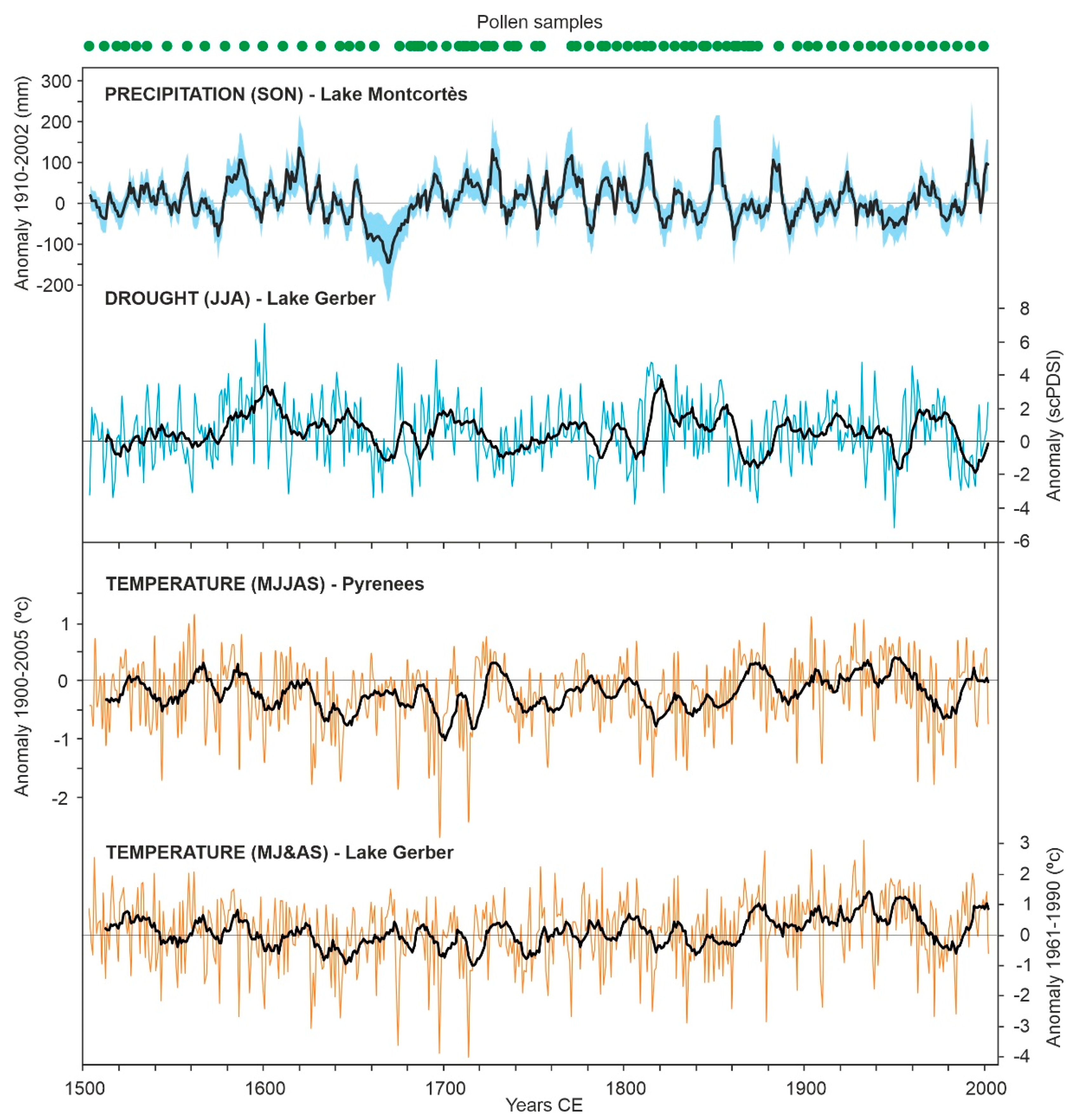
Figure 6.
Paleoclimatic reconstructions inferred from pollen-independent proxies in the sediments of Lake Montcortès and other Pyrenean lakes. Values are provided in terms of anomalies with respect to the instrumental records of the periods indicated. In the case of summer drought intensity, the anomalies are relative to the self-calibrated Palmer drought indices (scPDSIs) for the Mediterranean region (see the original reference). Samples for pollen analysis are indicated in the upper part for reference. Precipitation (Lake Montocrtès) after ref. [46], drought (Lake Gerber) after ref. [44], upper temperature series (Pyrenees) after ref. [43] and lower temperature series (Lake Gerber) after ref. [44]. SON, September–October–November; JJA, June–July–August; MJJAS, May–June–July–August–September; MJ&AS, May–June, and August–September.

Figure 7.
Gaussian curve displaying a hypothetical unimodal response of a species with respect to an environmental variable. The gray bands represent subranges of the environmental variable where the response may appear nearly linear. Redrawn and modified from [54].
Figure 7.
Gaussian curve displaying a hypothetical unimodal response of a species with respect to an environmental variable. The gray bands represent subranges of the environmental variable where the response may appear nearly linear. Redrawn and modified from [54].

Figure 8.
Forest taxa with significant Gaussian responses to climatic reconstructions.

Figure 9.
Forest taxa with significant Gaussian responses to anthropogenic drivers.

Figure 10.
Examples of forest taxa with nonsignificant and/or misleading responses to external factors.
Figure 10.
Examples of forest taxa with nonsignificant and/or misleading responses to external factors.

Figure 11.
Response lags of the major forest components with respect to the climatic drivers. Only linear correlations have been considered in this case. The dotted lines represent the significant correlation values at p < 0.05, which show a slow increase as the number of samples decreases.
Figure 11.
Response lags of the major forest components with respect to the climatic drivers. Only linear correlations have been considered in this case. The dotted lines represent the significant correlation values at p < 0.05, which show a slow increase as the number of samples decreases.

Figure 12.
Cluster analysis of forest-tree pollen elements performed using the Pearson coefficient and the UPGMA clustering approach [57,58]. The dominant taxa of each forest assemblage are in bold. A1, assemblage 1; A2, assemblage 2; A3, assemblage 3.

Figure 13.
Successional variations in the forest assemblages defined in Figure 8 and rate of change. SED, standardized Euclidean distance. Rate of change values have been calculated using all taxa of Figure 4.

Figure 14.
Euclidean biplot of the scores of the first three components of the PCA: PC1–PC2 in the upper panel and PC1–PC3 in the lower panel (see Table 3 for details on these components). Vectors corresponding to forest taxa other than Quercus, Pinus, and Betula are too small to be represented. The associations of forest taxa defined previously by cluster analysis (Figure 13) have been represented near the scores of their dominant taxa and are used as attraction domains [60]. Samples have been depicted as dots using a color code that indicates the century to which they belong. Colored arrows represent the approximate successional trajectories for each century obtained using the ages of samples and the same color code.

Figure 15.
Scatter plot generated using the scores of the significant axes obtained in the RDA. Black arrows are the environmental variables, open diamonds are the selected taxa (B, Betula; P, Pinus; Qd, deciduous Quercus; Qe, evergreen Quercus), and colored dots are the sample scores, using the same color code as in Figure 14. The gray arrow indicates the general successional trends. Samples corresponding to the phase of maximum deforestation (1740–1770 CE; Figure 4) are connected by a dark-yellow line.

Figure 16.
Successional trends of Montcortès forests, as represented by the main successional stages (in bubbles), the external drivers analyzed in this paper (brown text), and the information from historical documentation (green text). Centuries are indicated by blue text.
Figure 16.
Successional trends of Montcortès forests, as represented by the main successional stages (in bubbles), the external drivers analyzed in this paper (brown text), and the information from historical documentation (green text). Centuries are indicated by blue text.


Table 1.
Temporal resolution of the available vegetation reconstructions using pollen analysis in the central Iberian Pyrenees (Figure 1). L, lake; B, peat bog; A, abbreviations; E, elevation; AR, age range; NS, number of samples; YS, years per sampling interval.
Table 1.
Temporal resolution of the available vegetation reconstructions using pollen analysis in the central Iberian Pyrenees (Figure 1). L, lake; B, peat bog; A, abbreviations; E, elevation; AR, age range; NS, number of samples; YS, years per sampling interval.
| Sites | A | E (m) | AR (yr) | NS | YS | Resolution | References |
|---|---|---|---|---|---|---|---|
| Marboré (L) | Mb | 2612 | 15,000 | 80 | 188 | Bicentennial | [11] |
| Forcat (L) | Ft | 2531 | 9500 | 105 | 90 | Centennial | [12] |
| Estany Blau (L) | EB | 2471 | 1200 | 40 | 30 | Multidecadal | [12] |
| Serra Mitjana (B) | SM | 2406 | 1500 | 15 | 100 | Centennial | [13] |
| Riu dels Orris (B) | RO | 2390 | 8000 | 60 | 133 | Centennial | [14] |
| Orris del Seut (B) | OS | 2300 | 3700 | 32 | 116 | Centennial | [14] |
| Estanilles (B) | Et | 2247 | 12,000 | 90 | 133 | Centennial | [15] |
| Redon (L) | Rn | 2240 | 10,000 | 130 | 77 | Subcentennial | [16,17] |
| Planells de Perafita (B) | PP | 2240 | 10,000 | 50 | 200 | Bicentennial | [12] |
| Bosc dels Estanyons (B) | BE | 2180 | 12,000 | 90 | 133 | Centennial | [14,18] |
| Ibón de las Ranas (L) | IR | 2092 | 10,000 | 40 | 250 | Bicentennial | [19] |
| Pradell (B) | Pd | 1975 | 1400 | 37 | 38 | Multidecadal | [20] |
| Sant Maurici (L) | Ma | 1914 | 2000 | 71 | 28 | Multidecadal | [21] |
| Basa de la Mora (L) | BM | 1914 | 15,000 | 140 | 107 | Centennial | [22] |
| Bassa Nera (B) | BN | 1891 | 7000 | 110 | 64 | Subcentennial | [23,24] |
| Coma de Burg (L) | CB | 1821 | 10,000 | 70 | 143 | Centennial | [25] |
| Tramacastilla (L) | Tm | 1668 | 15,000 | 150 | 100 | Centennial | [19] |
| Llebreta (L) | Ll | 1619 | 3600 | 240 | 15 | Bidecadal | [26] |
| Prats de Vila (B) | PV | 1150 | 2200 | 30 | 73 | Subcentennial | [27] |
| Estanya (L) | Es | 670 | 20,000 | 65 | 308 | Multicentennial | [28,29] |
Table 2.
Linear (normal font) and exponential (italics) correlation coefficients between the forest taxa and the external drivers that were significant in the Gaussian response analysis (Figure 10 and Figure 11). In most significant cases, the linear and exponential models showed very similar correlation coefficients, and the higher values were chosen. Correlations significant at p < 0.05 are in bold.
| Quercus (d) | Betula | Quercus (e) | Pinus | |
|---|---|---|---|---|
| Temp1 | 0.374 | 0.251 | 0.104 | −0.014 |
| Temp2 | 0.322 | 0.133 | 0.118 | −0.180 |
| PPT | −0.089 | −0.288 | 0.231 | −0.039 |
| DGT | −0.036 | −0.064 | −0.225 | −0.032 |
| Olea | 0.220 | 0.292 | −0.195 | −0.408 |
| Cereals | −0.325 | −0.207 | −0.367 | −0.343 |
| Sporormiella | −0.330 | 0.170 | −0.295 | −0.334 |
| Charcoal | −0.402 | 0.064 | −0.293 | −0.114 |
Table 3.
PCA variable loadings and variance explained by the three significant components (PC1 to PC3), according to Kaiser’s rule [62]. The highest loadings are in bold.
Table 3.
PCA variable loadings and variance explained by the three significant components (PC1 to PC3), according to Kaiser’s rule [62]. The highest loadings are in bold.
| PC1 | PC2 | PC3 | |
|---|---|---|---|
| Quercus (d) | −0.082 | 0.452 | 0.841 |
| Betula | −0.068 | 0.019 | 0.285 |
| Cornus | −0.004 | 0.014 | −0.013 |
| Salix | −0.012 | −0.030 | 0.006 |
| Alnus | 0.008 | −0.001 | 0.021 |
| Tilia | −0.002 | 0.004 | −0.005 |
| Quercus (e) | 0.120 | 0.886 | −0.414 |
| Corylus | 0.006 | 0.068 | −0.123 |
| Fagus | 0.013 | 0.006 | −0.057 |
| Abies | 0.000 | 0.003 | −0.005 |
| Pinus | 0.987 | −0.070 | 0.142 |
| Morus | 0.009 | 0.004 | −0.007 |
| Ulmus | 0.020 | 0.019 | 0.001 |
| Populus | 0.002 | 0.006 | 0.000 |
| Fraxinus | 0.004 | −0.001 | −0.008 |
| Cumulative variance (%) | 52.329 | 76.639 | 91.075 |
Publisher’s Note: MDPI stays neutral with regard to jurisdictional claims in published maps and institutional affiliations. |
© 2022 by the authors. Licensee MDPI, Basel, Switzerland. This article is an open access article distributed under the terms and conditions of the Creative Commons Attribution (CC BY) license (https://creativecommons.org/licenses/by/4.0/).
Share and Cite
MDPI and ACS Style
Rull, V.; Vegas-Vilarrúbia, T. Climatic and Anthropogenic Drivers of Forest Succession in the Iberian Pyrenees during the Last 500 Years: A Statistical Approach. Forests 2022, 13, 622. https://0-doi-org.brum.beds.ac.uk/10.3390/f13040622
AMA Style
Rull V, Vegas-Vilarrúbia T. Climatic and Anthropogenic Drivers of Forest Succession in the Iberian Pyrenees during the Last 500 Years: A Statistical Approach. Forests. 2022; 13(4):622. https://0-doi-org.brum.beds.ac.uk/10.3390/f13040622
Chicago/Turabian StyleRull, Valentí, and Teresa Vegas-Vilarrúbia. 2022. "Climatic and Anthropogenic Drivers of Forest Succession in the Iberian Pyrenees during the Last 500 Years: A Statistical Approach" Forests 13, no. 4: 622. https://0-doi-org.brum.beds.ac.uk/10.3390/f13040622
Note that from the first issue of 2016, this journal uses article numbers instead of page numbers. See further details here.