
Computation of Strip Road Networks Based on Harvester Location Data


Metsäteho Oy, Vernissakatu 1, 01300 Vantaa, Finland
*
Author to whom correspondence should be addressed.
Forests 2022, 13(5), 782; https://0-doi-org.brum.beds.ac.uk/10.3390/f13050782
Submission received: 31 March 2022
/
Revised: 12 May 2022
/
Accepted: 13 May 2022
/
Published: 18 May 2022
(This article belongs to the Special Issue Recent Advances in Wood Harvesting, Timber Logistics and Road Planning)
Abstract
:The location information of strip roads in thinnings and the numerical variables of strip roads are one aspect of timber harvest quality information. The ideal of automatic quality management for mechanized logging is that the quality of the harvest is calculated and reported based on data collected by forest machines. At present, quality data is collected by means of laborious, manual, field-based, post-harvest measurements. The aim of this study was to develop an automatic method to compute the strip roads of the harvested stands after harvesting, based on the stem-specific location data of the harvester. Subsequently, the strip road variables were computed from the strip road networks. The computed strip road networks were validated with 21 manually recorded field references. The method was also applied to operational stand data, including 544 harvested stands collected from Southern Finland. The results showed that the computation method produces well-located, stand-specific strip road networks from which strip road variables can be accurately determined, covering the whole stand. Thus, the method promotes the automation of quality management and reporting. The computed strip road networks can also support harvester operator work during the harvesting and, later, the automation of harvesting operations.
1. Introduction
Cut-to-length (CTL) thinning operations are performed using strip roads cut through the forest [1]. A harvester operator plans the directions of the strip roads and cuts them through the area to be thinned during the work. The aim for the average strip road spacing is to be 20 m or more [2]. The length of the boom of the harvester is typically 9–11 m, which means that the area between the strip roads can be reached from the strip roads, and the harvester does not have to make any kind of short spur trails to the area between the strip roads. The default is that the forwarder also uses the same strip roads as the harvester in the forwarding phase.
The goodness of a strip road plan and its implementation is assessed on the basis of the strip road density (m/ha), the average strip road spacing (m) and the strip road width (m). The width of the strip road should not be too wide, because the growth space of the trees will be otherwise be lost for the strip road. On the other hand, the strip road cannot be too narrow, because the machines working on the strip road can easily damage the trees at the side of the strip road. The recommended width of a strip road is 4–4.5 m [2]. It is worth noting that the area of the strip road network represents the area needed for the harvester and forwarder to move on the stand, and the movements are limited by the strip road edge trees [3]. It differs from the contribution of the strip road network’s area to the wood-productive area of the stand. The loss of wood-productive area along a strip road is typically less than 2 m wide [4].
Strip road spacing is also an important part of the goodness of the strip road implementation. Strip road spacing is defined as the distance between the center lines of two parallel strip roads [2]. Too short strip road spacing wastes tree growth space under the strip road network, and too wide strip road spacing, in turn, leads to the use of spur trails and a decrease in the productivity of harvesting. In thinnings, the limit for incorrect spacing is 19 m or less [5]. Typically, strip road density correlates with strip road spacing. Therefore, from the point of view of profitable forestry, it is important to implement strip road networks according to recommendations.
In Finland, the goodness of a strip road network is measured in regional monitoring based on random stand sampling where a certain number of stands is selected for monitoring in a certain geographical area [6]. In addition, the wood procurement units of the forest companies also make control measurements on their harvesting sites and give feedback to the harvesting contractors or harvester operators. Regional monitoring is conducted continuously, and the results are published once a year. Monitoring by forest companies occurs soon after harvesting and it can be used for instant harvester operator feedback.
Typically, when a stand is selected for manual control measurement, a systematic network of sample plots is used to determine the characteristics of the strip road [5]. However, manual measurements of the strip road network are time consuming and expensive. In addition, a sample-based assessment is not comprehensive: it includes samples of individual stands that are generalized to represent the success of harvesting throughout the whole geographical area. In addition, if the aim is to improve harvester operator quality of work, then feedback should be more real-time, provided on every cut stand.
To tackle the challenge of the laborious field measurements involved in obtaining data on harvest quality, there is a need for comprehensive, automated and more real-time strip road network information. Such information would benefit both the quality monitoring of harvesting work and forwarder operator guidance, which could become part of operative routines. In the long run, computed strip road networks facilitate automation of forwarder work, or automation of the next harvesting operation in subsequent thinnings by assisting the operator. Comprehensiveness of the data on strip road variables in time and geography is a prerequisite for large-scale verification of the realized harvesting quality.
Early research on strip roads discussed the concept of strip road width, area and its influence on tree growth, e.g., [4,7,8]. These studies were continued by measuring and predicting rut depths on strip roads caused by forest machines [9,10]. The trafficability of the strip roads has been determined on the basis of the spatial information [11,12]. Recently, research has focused on the preplanning of main extraction roads on stands by using geospatial methods. The aim is to assist the forest machine operators in placing the main extraction roads [13,14,15,16,17].
In this work, a novel approach to generate strip road information for quality assessment purposes is proposed, utilizing the location information of harvesters. In contrast to earlier research related to the preplanning of main extraction routes, the current method concentrates on obtaining information on the realized strip road network after harvesting.
Determination of a strip road network via geoprocessing computations requires a sufficient number of location point observations of the harvester route. The determination of harvester locations is commonly based on global satellite navigation system (GNSS) technology, which requires harvesters to have a GNSS receiver. The receiver is usually placed upon the roof of the harvester, where the best possible connection to the satellites can be made in forest circumstances. The location accuracy of typical GNSS receivers used on harvesters varies from a few to several meters under the forest canopy [18,19]. Location points can be saved to files according to the forest machine standard StanForD [20]. In Finland, approximately 90% of operative harvesters use the StanForD standard [21].
Currently in Finland, there are two automatic recording methods for harvester locations. In the first method, the location points of the harvester are stored directly through a forest company’s wood procurement system by means of the so-called “recording function” (Figure 1a). A new location point is saved whenever the spatial or temporal distance from the previous location point becomes large enough, after which, all the points are converted into a route line. In this method, using the StanForD2010 standard, the strip road recorded by the harvester can be saved into the tracking structure of an HPR file, whereas the forwarder records its driving routes into the similar tracking structure of an FPR file [20]. In this method, there is variation between company systems and, therefore, in the details of the recording, such as sampling frequency, basis of recordings, positioning accuracy, and raw data processing, which may have been performed in the intermediate stages. The recorded route enables visualization of the rough location of strip road network afterwards, but the recording is often too sparse to determine the more detailed location of strip roads.
The second method is to store the location of the harvester for every processed stem (Figure 1b). When a stem is felled and processed by a harvester, the location information is stored automatically in a stem (STM) or harvester production (HPR) file, following the StanForD2010 standard [20]. It is worth noting that the location of the harvester is stored instead of the location of the harvested stem, as the GNSS receiver is located on the roof of the machine. With this storage method, the locations of the harvester are clustered into sets of locations on the map, as several stems are typically felled from the same working location without the harvester driving between the stems to be felled. The location of the harvester can vary from a few meters to over 10 m depending on the accuracy of the receiver [22].
When considering the computation of strip road networks based on the stored locations of harvesters, some common challenges are identified for the two recording methods of locations. The harvester sometimes drives the same strip road back and forth several times. For example, when changing operator shifts, the harvester is typically driven to a roadside storage location for service. This kind of operative driving causes, in the first route recording method, the total length of the recorded strip road to not be directly usable, since the harvester records all the driving times separately. In the second, stem-wise-based location storing method, only one strip road route is desired for the computed strip road network at each location, regardless of how many times a certain strip road has been driven through.
Positioning inaccuracy in GNSS also affects both location recording methods. In general, the satellite positioning technique sometimes shifts the apparent GNSS locations of consecutive observations due to terrain obstacles or the movement of satellites, resulting a systematic local deviation of locations. Pointwise inaccuracy causes the location points to jump back and forth by several meters in relation to the real position of the harvester. In sparse sampling of the first method, the location accuracy of the recorded strip road varies along the accuracy of the single location points. In the second location recording method, the felling order of the stems cannot be used to directly calculate the strip road. However, the stem numbers, i.e., information on the progress of the harvesting work, generally helps to form the strip roads.
Strip road computation based on HPR data is also a relevant part of the software called hprGallring, which is developed by Skogforsk in Sweden [23]. The software is used to estimate harvesting quality and assist harvester operators at thinnings. Köppler [24] presents details on how strip roads are computed in hprGallring. They obtained somewhat shorter computed strip road lengths than the references. In addition, they found the following challenges in their strip road generation algorithm:
- The strip road crossings were not included in the strip road network.
- The algorithm failed to unite the strip road parts of the straight strip road.
- Sometimes, parallel, duplicate strip road parts were generated beside the actual strip road network.
- Strip roads were partly formed outside the stand.
Here, the first two points provide a reason to produce topologically unified strip road networks. The observation of the third bullet refers to the issue of several separate driving times being recorded on the same strip roads.
The main aim of this study was to develop a method for computing strip roads based on stem-wise harvester location data, taking into account the identified properties of the data and the desired strip road networks. The focus was on determining the location of the strip road network as correctly as possible. The locations of the computed networks were validated with manual field recordings by using a comparison tool of strip road networks developed for the purpose. The descriptive variables of the strip road networks could then be calculated from the location-validated network. To calculate strip road network variables, two alternative tools for determining strip road spacing are presented: one that mimics the quality control measurement performed in the field using ten sample points, and one that samples more densely through the whole strip road network.
2. Materials and Methods
The overall framework of assessing the harvesting quality in this work is presented in Figure 2, including both the manual strip road measurements in the forest and the automated approach. The aim of this work—developing an automated strip road computation method and the calculation of strip road variables—consists of several separate geoprocessing blocks that were run for the harvester data. The validation of the strip road generation is also shown in Figure 2. The arrows in the flow chart (Figure 2) show how the main lines in the available datasets were processed in this work.
2.1. Harvester Data
The harvester data of the study were recorded during operational logging from August 2015–September 2016. The harvesting sites were located in the Uusimaa region in Southern Finland (Figure 3), including various features of the landscape, nature and land use.
Six harvesters from three different machine manufacturers participated in the study. Four harvesters were from Ponsse (Vieremä, Finland), one from Komatsu Forest (Umeå, Sweden) and one from John Deere (Moline, IL, USA). The harvester data was collected from STM files and contained 455 harvested objects and 634,656 stems in total. A harvested object corresponds to an operational unit of field work in wood procurement. One harvested object can include many smaller harvesting sites with the same harvesting method, to which forest machines are relocated from the previous harvesting area/object.
The STM files contained the location points of the harvester for each felled stem. The identifiers of the harvested object and the starting time of the object were also available. In addition, detailed information on stems, e.g., dimension measurements and tree species, was stored in the STM files.
The stem-wise harvester coordinates and object data were extracted from the STM files. The information was inserted into a relation database, from which it was further exported into a geographical information system program, QGIS (Open Source Geospatial Foundation, [25]). The harvester data was originally recorded in the WGS84 (EPSG:4326) coordinate system, and the data was reprojected in the QGIS program into the Finnish metric coordinate system known as ETRS89/ETRS-TM35FIN (EPSG:3067). An automatically produced label identified the harvested objects (for details, see [22]). The stems were identified in the data by a unique, continuous “StemNumber” recorded by the harvester. Attribute StemNumber also represents the felling order of the stems.
However, the STM files do not contain the harvesting methods of the objects. For this reason, the harvesting method was separately obtained from the forest companies and manually added into the location data. It is worth noting that the HPR files, when compared to STM files, contained harvesting methods in their data accordant with the StanForD2010 standard [20] and could, therefore, be used as stand-alone data sources for strip road computation.
A harvested object is an operational unit of field work, compiled from site of wood procurement. One harvested object can include many harvested stands, which correspond to typical forest inventory stands and can be observed at the harvesting sites. In this work, the harvested stands were more useful than the harvested objects, since the strip road networks are, in practice, implemented at the marked stands, not at the harvested objects. In addition to several stands, harvested objects may contain stems harvested outside of the marked stands. Such stems are harvested from, e.g., external strip roads, which lead from stands to roadside storages.
To convert the harvested objects into harvested stands (the areas of the harvested sites), the stem-wise harvester data was run through an automated stand-delineation method by Metsäteho Oy [22]. This method converts the stem location datapoints of harvested objects into accurate polygon geometries of the harvested stands. One harvested object can turn into several separate harvested stands, depending on how the object was originally compiled. This method also separated external strip roads from stands for roadside storage, which were excluded in this work. Stem point classification, which also results from the stand-delineation method, indicated which stems were harvested from a certain stand and, thus, provided the stand-wise groups of stems. At the same time, the external strip road points were separated from the stem-wise data. Since they were not part of the stand itself, they were left out of the scope of the current work. The exclusion of these points helped to target the strip road computation for the area of the harvested stand. The stand-delineation method resulted, altogether, in 544 stands, which were delineated from 455 objects for the most common harvesting methods from the data of this study (see Table 1). The same stand area classification was used as in a previous publication [22].
In addition to the harvester location data, a dataset of strip road route recordings of harvesters was separately obtained from the forest companies. Those recordings partly covered the same harvesting sites as the STM files. However, they were not recorded according to the StanForD2010 standard; rather, they were delivered as individual geospatial information system files. The distance interval of this method recorded points that were too long for the accurate determination of strip road locations; for example, see Figure 1a, in which the average interval is 17.7 m.
2.2. The Reference Data
The reference strip road field data was collected in spring 2018, two years after the harvesting operations. Altogether, 21 first thinnings were recorded by walking along the middle lines of the strip roads with a mapping-grade GNSS receiver placed at a height of 2.5 m at the top of the mapping stick. A Trimble Geo 7X receiver (Trimble, Sunnyvale, CA, USA) with VRS H-Star correction was used, for which the accuracy estimated by the manufacturer is approximately 0.1 m in good conditions [26]. However, it is known from many studies [27,28,29] that, under a forest canopy, mapping-grade GNSS receivers are about 2–5 m accurate, and recreation-grade receivers 6–10 m accurate. The sampling interval of the receiver position was one second, which corresponded to a line node interval of approximately 1 m or less in the data. In practice, the strip road network was recorded in parts: the beginning and endpoints of certain strip road parts were estimated as realistically as possible. The Trimble Geo 7X receiver records a horizontal precision value for each location point. Based on these horizontal precision values, an average horizontal precision value was calculated for each thinning stand.
The reference harvesting sites were selected from the harvested stands of this study by the area of the stands. Only first thinnings were considered, since no previous strip roads should exist at those stands. An important requirement in the reference stands was also a good overall correspondence between the harvested stand (i.e., harvester data) and the realized outcome in the field. For example, certain strip roads, or even some parts of the stand that were harvested at the site, are sometimes not included in the harvester data. The shape of the reference stand was also considered: a network of strip roads was preferred rather than a couple of long, parallel strip road lines at the stand. After all, the stand area classes were rather evenly represented in the set of reference sites: 5, 4, 8 and 4 stands of 18, 8, 11 and 5 possible stands were included, respectively (see Table 1).
After the field work, the mapping-grade GNSS data was manually checked in the QGIS program. The dense sampling interval of the data and GNSS inaccuracy caused, to some extent, small loops in the line geometries. These loops had to be manually straightened. In some cases, the beginning/endpoints of the strip road parts were recorded notably outside of the stand, especially in the case of external strip roads leading to stands. For this reason, the external route parts that lay clearly outside of the marked stand were removed. The intervals of the line nodes of the reference recordings were manually adjusted to approximately 5–8 m per node interval, which roughly corresponds to the length of a typical harvester.
2.3. Strip Road Network Computation Method
The computation of the strip road network was a fully automated, four-phase geoprocessing method (Figure 4). The input data were the harvester location points of one harvested stand, obtained with the stand-delineation method. The points were averaged, and then the strip road sequences of the strip road were identified. Strip road lines for the sequences were produced, and finally, the lines were connected into a strip road network.
A pilot version of the computation method was implemented using Python geoprocessing scripts in the QGIS 2.14 program [25]. This environment also provided access to the spatial processing libraries SAGA [30] and Shapely [31].
2.3.1. Phase 1. Averaging of the Location Points
At first, all the raw location points of the HPR file were averaged to reduce the error from the GNSS positioning inaccuracy, which was present in each recorded location. The averaging was performed spatially, i.e., the points used in averaging were selected according to the distance from the study point. The selected points were searched for one study point at a time from the raw locations. Both the x and y coordinates were averaged arithmetically since the locations were reprojected into the Finnish metric coordinate system during preprocessing of the harvester data. The new, averaged locations of the study points were saved separately for further use. The intensity of the averaging was adjusted by the averaging radius. The value of the averaging radius was 3 m in final fellings and 4 m in thinnings when the GNSS positioning of the object was computationally estimated “more accurate” (see Appendix A in reference [22]). For objects where the computationally estimated GNSS accuracy was “less accurate”, the radius of the averaging was 12 m for all harvesting methods, depending on the harvesting method (see Appendix A in reference [22]).
The benefit of spatial averaging is that it was independent of the felling order of the stems as well as of separate driving times. This approach also allowed us to utilize single location points originating from the felling of a few stems while driving from the landing to and off the stand, e.g., for changing work shifts and refueling. Each recorded point provided information about the strip road’s location, as the harvester drove along the same strip road network in any case. Altogether, using all the datapoints improved the accuracy of the averaged datapoints and, further, the accuracy of the resulting strip road network with respect to the raw data. If averaging was performed based solely on the felling order, corresponding to one driving time, these single locations would either skew the averaged result or be excluded completely from the averaging. The problem of several different driving times was also recognized in [24], where duplicate lines appeared next to the strip road lines since the harvester had operated two times along the same strip road, but data from only one driving time was used to compute the strip road.
2.3.2. Phase 2. Identifying the Strip Road Sequences
The progress of harvesting work on the site was relevant background information for successful computation of the strip road networks. The progress depends on prevailing harvesting conditions, planning of forwarding and the personal preferences of the harvester operator.
Within one strip road sequence, the stem felling location points were often rearranged from the felling order (StemNumbers) due to GNSS positioning error. This appears when looking closely the StemNumbers of the points along the course of the strip road (Figure 5). However, the mutual distances of the points remained short enough, and that allowed us to identify the strip road sequences computationally from the harvester data. For this reason, the felling order of individual stems is not directly applicable to depicting the progress of the harvesting.
To that end, the concept of “strip road sequence” was created. The strip road sequence is a set of consecutively felled, averaged stem points that are close enough to each other (15 m) that they could have been harvested from the same strip road. Strip road sequences, therefore, provide somewhat coarse-grained but still adequate information on the progress of the work at the harvesting site.
In this phase, the strip road sequences were identified from the averaged point data. The points of each sequence were labeled by attribute.
2.3.3. Phase 3. Creating the Strip Road Lines for the Strip Road Sequences
The strip road lines were computed for each strip road sequence at a time. They already resembled the final result and formed the backbone of the complete strip road network that was obtained from the process. This phase ensured that only one strip road line was produced for a certain location, regardless of how many times the harvester drove or felled trees from that strip road sequence (cf. [24]). This feature was crucial for obtaining spatially “clean” strip road networks.
The strip road lines were drawn by creating single line segments for the entire strip road sequence. At first, the beginning point of the strip road sequence was determined by finding the furthest endpoints of the sequence. The following step was to find the next position, far enough in the strip road sequence to further smooth the GNSS inaccuracies that can still be, in some degree, present in averaged location data. The direction of the harvester’s movement was predicted to estimate the likely area in the search for the next point. When the next point was found from the proximity of the searching location, a line segment was added between the two points. Subsequently, the next new point was searched for, and the drawing proceeded iteratively, segment by segment, until the entire strip road sequence was gone through. The length of the created line segments was limited to 12 m, and no crossing to other lines was allowed. Limiting the maximum length of the segments helped the strip road line to follow better the datapoints, e.g., in curves of the strip roads.
In drawing the lines, it was assumed that the harvester could turn its driving direction only rather slightly when driving along the strip road. This assumption relates, to some degree, to Kalman filtering [32], where the trajectory of a vehicle is predicted and updated with dynamic location measurements. However, in this case, the time dimension becomes irrelevant, and only the locations mattered in obtaining the spatial features of the strip roads. The uncertainty of the GNSS location measurements, explicitly present in Kalman filtering, was handled in this work indirectly by averaging the raw location points of the harvester and keeping the averaged results as the “certain” positions for simplicity.
Spur trails were produced together with strip road lines. A spur trail was added perpendicularly to the strip road line if some averaged points were located further than 6 m away at the side of the computed strip road. The selected value of the spur trail length was determined visually and reflects the length of the harvester, taking into account that the spur trail was identified from the averaged points. This way, the spur trail occurred when the harvester drove away from the strip road, not when the harvester barely turned its front or rear part outside of the strip road. After all the strip road lines of the sequences were ready, the spur trails were redirected to the nearest strip road line. This improved the outcome: the spur trails became more realistic and the effects of single erroneous locations and computational artefacts diminished.
2.3.4. Phase 4. Merging of the Strip Road Network
At the last phase, the separate strip road lines were connected into a strip road network. Here, the strip road network describes the spatial layout of the routes at the stands—it does not provide information on how many times a strip road was driven through during harvesting work.
To compile the strip road network, the endpoints of the strip road lines were identified. Often, some single points remained outside the vicinity of the strip road lines. They lay so far from the other points that spatial averaging did not alter their location, and they did not connect directly to the strip road lines. In the merging phase, these single points were collected into the strip road network. If the distance of such a point to a strip road endpoint was within 6 to 15 m, the strip road line was continued until that single point. The strip road endpoints were then updated.
For the merging, the mutual distances of the strip road endpoints were studied two points at a time. If the distance between two endpoints was less than 18 m, a line segment was created between them. The limit distance allowed us to couple together two single strip road endpoints whose location was not altered in the spatial averaging. One endpoint could be joined to only one other endpoint in order to avoid excessive connections in the resulting strip road network. The strip road lines may not be completely connected to each other in the network. However, in reality, the harvester also drove, somehow, to nonconnected sequences of the strip road network. It is also possible that the method sometimes generated strip road endpoint connections that the harvester did not drive along. Information about where the harvester actually drove between the strip road endpoints was not available in the harvester data based on felled stems.
2.4. Calculation of Strip Road Variables
In the sections below, the methodology and all calculated variables and comparisons of this work are presented. The strip road variables were calculated in a similar manner to both reference and computed strip roads networks.
2.4.1. Strip Road Variables from Whole Stand
The following numerical variables were calculated for the computed strip road networks (units given in parentheses):
- -
- The total length and density of the strip road network (m, m/ha);
- -
- The relative area of the strip road network of the stand area, assuming a constant width (4.5 m) of strip roads (%);
- -
- The average strip road spacing (m).
The area of the harvested stand was needed in these calculations, and it was obtained from the automated stand delineation. The total length of the strip road network was obtained directly from the line geometries of the network and it was converted into hectare-wise value by the stand area.
The area of the strip road network was obtained by buffering the line geometry with constant width and then determining the area of buffered geometry. In this study, a strip road width of 4.5 m was used. The relative area of the strip road network on the stand was calculated using the area of the harvested stand.
The average strip road spacing and its standard deviation (SD) were calculated extensively for the whole computed strip road network. The average strip road spacing means perpendicular distance between two parallel strip road center lines. The spacing of each non-crossing line segment was obtained by measuring the perpendicular distances from the center point of the line segment to nearest adjacent strip roads (Figure 6). If an adjacent strip road was found at both sides of the line segment under study, the average of the two distance values was registered as the strip road spacing for that segment. In cases of finding only one adjacent strip road, that distance value was the strip road spacing for that line segment. A maximum value of distance was used to limit the range from which the adjacent strip roads were considered in this calculation.
To exclude crossings from the strip road spacing calculation, they were automatically identified and marked, since their strip road spacing was not realistic. In addition, the location inaccuracies at crossings often appeared to be somewhat larger than in the middle of strip road sequences. The reason for this probably originates from datapoints recorded at different driving times that were not completely overlapping on the map. Typically, more moving space is needed in crossings for forest machines, which enables slightly different driving locations.
2.4.2. Automation of Manual Control Measurements with Systematic Sampling Plots
The systematic sampling of the strip road networks according to forest management recommendations [5] typically takes place in the field, when the harvesting site is measured manually for quality control. In this work, the traditional sampling method was automated by implementing it as a geoprocessing script in the QGIS program. The input data of the automated sampling measurement are stand geometries and strip road networks. The detailed stages of the process are explained below.
At first, the longest diagonal within the stand polygon was determined (Figure 6). For that, the boundary line of the stand polygon was split into short segments of constant length. The whole boundary was gone through when searching for the longest perpendicular diagonal line; inner boundaries of polygons were neglected. After this diagonal was found, the exact positions of the diagonal endpoints were allowed to slightly shift in both directions to find the longest diagonal, i.e., sampling line, which is not necessarily perpendicular to the stand boundary.
The crossings of the sampling line and the strip road network were studied to ensure sampling of at least two different interjacent areas between strip roads. If this condition was met, 10 sampling points with equal intervals were set along the sampling line. The interval of points was 1/11th of the sampling line’s length to exclude areas near stand boundaries.
Subsequently, the strip road spacings at the sampling points were measured with the help of another line geometry. This line was searched for in order to pass through the center of the sampling point and, at the same time, be the shortest line to adjacent strip roads (see also Figure 2 of [5]). Then, the goodness of the sampling geometry was studied by the following conditions: The segments of the nearest strip road lines could deviate, at most, by 35 degrees; the shortest line could be located at an angle under 30 degrees with respect to the strip road segments; the total length of the shortest line had to remain under 35 m; and both the strip road segments could not be crossings of the network. If all these conditions were met, the sampling point was accepted, and the strip road spacing value for the sampling point was determined as a length of the shortest line.
In the case of obtaining less than 10 accepted observations from the diagonal sampling line, additional sample points were generated randomly at the sides of the sampling line one by one until 10 samples were obtained. The generated points had to be located in a two-dimensional grid in the stand with the same intervals to other points (Figure 6). A zone of 20 m inwards from the stand boundary was, however, forbidden from locating the generated sampling points. If all the possible sampling grid locations were looped through without gaining 10 accepted samples, the sampling was ended. The stand-wise results included the average strip road spacing of samples, its standard deviation, the number of accepted samples, as well as sample point intervals.
The automation of the quality control measurement allowed us to compare its results with the strip road spacings sampled from the whole stand. The spacing values of the computational and systematic sampling network were compared statistically using the Mann–Whitney U-test (M-W) with SPSS version 26 (IBM, Armonk, NY, USA), because the number of observations was small and not normally distributed. For analyses, the significance level was set at p < 0.05. The automated systematic sampling could not be performed for all stands, for example, if the stand was very small or the strip road network was irregular.
2.5. Validation of Strip Road Networks
The validity of the computed strip road network to the GNSS recorded field reference was studied by comparing the spatial correspondence of the two networks in detail. In Section 2.3, attention was paid to generating the strip road lines to the averaged, best possible locations with respect to the harvester data. Therefore, the validation essentially concerns indicating the goodness of the GNSS positioning of the harvester as well as detecting possible location deviations caused by the strip road computation method.
An example of a systematic GNSS positioning error in harvester locations within one stand can be visually observed in Figure 7. In some parts of the stand, the location points lie, on average, in balance over the reference strip road network line, while at other parts of the stand, the points are on the side of the reference network line.
To find possible displacements in the strip roads, the counterparts of the reference and computed strip road networks were compared by sampling the line segments of the computed strip road network, in a similar fashion to determining the strip road spacings (see Section 2.4.1). However, here, the perpendicular distance to the reference network was measured for each sampling segment, representing the displacement of the computed strip road.
The stand-level spatial match was estimated from the displacement distance values by calculating the root mean square error (RMSE) of displacements:
where di = ith displacement distance value, and N is the total number of the distance values. The larger the RMSE value is, the more the locations of the strip road networks deviate from each other.
To quantitatively study the local systematic displacements of the computed strip roads at the sub-stand level, the displacement distances were averaged for the individual strip road sequences that form the network. A minimum requirement of five distance observations per strip road sequence was set for averaging. This helped to target the analysis for longer continuous strip road sequences, which are typical for operational harvesting work.
For strip road sequences, displacement distance values close to zero indicate that the computed strip road is rather evenly distributed on both sides of the reference line (see Figure 7). Subsequently, the computed strip road can be close to the reference, indicating good correspondence. Alternatively, it can be displaced further from the reference in such a manner that deviations cancel each other in average; i.e., the computed strip road is at different sides of the reference. If the value of the average displacement distance is, for example, several meters, the computed strip road is systematically displaced to one side of the reference.
In addition to validating the spatial correspondence of the strip road networks, the strip road variables were calculated. The lengths were converted into relative lengths by dividing the length of the computed strip road network by the length of the reference strip road network. The average spacings were compared by using the values that were obtained as described in Section 2.4.1.
3. Results
This section has two parts. First, the comparison of the results of the computed strip road networks to the field-recorded reference strip roads are detailed. Then, the characteristic variables for all strip road networks of the whole harvester dataset are presented.
3.1. The Correspondence of the Computed and Reference Strip Road Networks
The spatial accuracy of the computed strip road networks was determined by comparing the result networks to the field recorded strip roads of 21 reference sites from first thinning stands. The most important results are presented below, and all the results are compiled in Table 2.
Overall, the computed strip road networks corresponded well with the references (Figure 8; see also Table 2). The spatial accuracy of the results was mainly good. The average RMSE of the displacement distances of the strip road networks was 2.7 m, which means that, in this context of the GNSS positioning of harvesters, local displacements from the reference networks were observed at certain strip road sequences. The average of horizontal precision values for all 21 reference thinnings was 0.62 m.
The total lengths of the strip road networks corresponded well to the reference lengths. The relative average length of the strip road networks was 106.5% (Figure 9). The results show that, when the RMSE value is small, the length of the computed strip road is also close to the length of the reference strip road network. This finding indicates that when the location of the computed strip road corresponds well to the reference, the total length is also reproduced well from the network.
The stand-wise average strip road spacings were calculated for both the computed strip road networks and the reference strip roads. The difference was then obtained by subtracting the average strip road spacings. The results are presented for all 21 stands in Figure 10. The average difference of the strip road spacings in this data was 0.5 m. The larger stand size improves the correspondence of the calculated average strip road spacing with respect to the average spacing of the reference strip road network (Figure 10). For stands that had fewer displacements in the computed strip road networks, the average spacings were also more accurately obtained. Example stands are shown in Figure 11.
3.2. The Strip Road Variables of the Whole Harvester Data
In the whole harvester data, the strip road variables were managed to calculate for 517 out of 544 stands. The results of the whole data are presented in Table 3, averaged separately for thinnings (here including both first and later thinnings) and regeneration fellings (clear cuttings, seed tree and shelter tree cuttings). The results are separately presented for different stand area classes in Table 3. Additionally, the stand-wise average strip road spacings of the dataset are presented in Figure 12. The sampling densities of the strip road spacing at stands varied roughly within 50 to 80 sample locations per hectare; for average sampling densities in stand area classes, see Table 3.
The average strip road spacing for all thinnings was 19.4 m and 17.1 m for all regeneration fellings when sampled from the whole strip road network, and 21.4 m and 18.6 m, respectively, when systematically sampled, similar to the quality control measurement described in Section 2.4.2. Note that the number of stands in Table 3 is smaller than in Table 1, since the strip road network and its variables could not be determined for all stands.
The results indicated that the variation of the strip road spacings depends on the stand size for both sampling alternatives. At stands below 0.75 ha, the strip road spacings vary greatly (Figure 12); some of the stand-wise averages are clearly not within a reasonable range of values. For stands over 0.75 ha, the variation of the strip road spacings decreased notably, and the results better represent the properties of the computed strip road network. Visual inspection of the computed strip road networks supports these findings.
The automated systematic sampling of 10 sample plots, which, in practice, correspond to the quality control measurement in the field, resulted in larger than average strip road spacings than the sampling of the whole strip road network (Table 3). The average spacing values and the systematically sampled spacing values of the whole computed strip road networks differed statistically from each other in thinnings (M-W, p < 0.001), final fellings (M-W, p < 0.001) and in all stands together (M-W, p < 0.001). The spacings are, however, consistent with each other, as can be seen in Figure 13. Pearson’s correlation coefficient of the two spacing values in thinnings was 0.515 (p < 0.01); in final fellings 0.584 (p < 0.01); and for all stands together, 0.611 (p < 0.01). The stand-wise variation of the systematically sampled spacings is larger than in sampling of the whole strip road network.
Automated systematic sampling could not be performed for 25 stands (14%) under 0.75 ha due to the small size or shape of the stand or irregularity of the strip road network. Additionally, the average numbers of the accepted sampling points are clearly lower for stands under 0.75 ha than for the other stand area classes.
The representativeness of the reference dataset can be observed from the results in Table 3. The strip road densities (m/ha) in first thinnings were very similar in all area classes. The average strip road spacings of reference stands were slightly larger than in the whole harvester data. This is assumed to originate from selection of the reference stands, where all the stand area classes were evenly represented, whereas in the harvester dataset, the number of smallest stands (area under 0.75 ha) was larger. With regard to the smallest stands, the results of the automatically calculated strip road spacings have lower reliability than larger stands, as discussed above, and the stand shapes and strip road networks can be more irregular than those in the larger stands.
4. Discussion
In this work, an automated method to compute stand-wise strip road networks from operational stem-wise harvester location datapoints was presented. The computed strip road networks provide detailed information of the locations of strip roads in the harvested stands. They also allowed us to extensively determine the strip road variables for the whole stand. The benefit of this approach is that the strip road variables, obtained from the computed strip road networks, are mutually comparable, since they are independent of the harvester brand or the settings of the strip road recordings. As such, the current recordings of strip road routes by harvesters cannot be used to estimate the length of the strip road network, because their sampling density is generally very low compared to the stem-wise data, and recording settings vary in the background. Moreover, the recordings also include all back and forth driving times at the stand.
To validate the computed strip road networks, their locations were compared, in a detailed manner, to the actual reference networks. The results indicated that the location accuracy of the computed strip roads is good in general. One aim of the work was to locate the computed strip road networks well enough that the calculation of the variables can be performed with good accuracy. In accordance with this, the total lengths of the strip road networks corresponded well to the references. The average strip road spacings were also quite well reproduced from the computed networks with respect to the references.
Some local displacements were observed in the computed strip road networks, which affected the average strip road spacings to some degree. The correctness of the location depends on several factors: the GNSS accuracy of the harvester, the GNSS satellite geometry of the locating time, the features of the terrain at the harvesting site, the working order of the harvesting and the parameter values of the strip road computation method. Further, the overall level of GNSS accuracy depends, indirectly, on the harvester brand, model and age.
Many environmental factors are known to affect location measurements under tree canopies [29,33,34]. For this reason, the reference strip road networks may have contained errors. In the study of Purfürst [33], the horizontal precision value of under-canopy measurements was 2.49 m (0.62 m in this study) using a similar Trimble Geo 7X receiver. It is, therefore, obvious that positioning errors exist in the reference recordings, and they influence the results. However, their impact is estimated to be minor, as the overall level of accuracy for forest machine work is sufficient. Some details of the strip road network, such as short spur trails, may have remained unobserved in the field. The collection of the reference data was limited to first thinnings in order to avoid disturbances of previously existing strip roads at the harvesting sites.
The results of the whole harvester dataset showed that the average strip road spacing is different for thinnings and regeneration fellings. In thinnings, the compliance to the recommended strip road variable values was clearly observed. Based on the results, it is obvious that the reliability of the computed strip road results depends on the stand size. This relates to difficulties in placing regular strip road networks in small stands, even during harvesting, as well as computationally obtaining the details of such networks. For stands over 0.75 ha, the automated strip road computing method and calculation of the variables worked well. The lower reliability of small stands is not considered a problem because, according to inspection guidelines of harvesting quality, strip road spacing is measured only on stands with an area of at least one hectare. Additionally, the shape of the inspected stands has to allow for the implementation of a regular strip road network, and at least 600 trees per hectare have to remain after harvesting [5].
The applicability of the reference dataset was studied with respect to the whole harvester data. The reference data concentrated on stands larger than 0.75 ha and represented the harvester dataset quite well. It is also relevant to consider that stands under 0.75 ha have lower reliability for the calculated strip road variables, which supports the representativeness of the selected reference stands.
In this study, the average strip road spacing was calculated by densely sampling the computed strip road network of the whole stand. This contrasts with the typical manual measurement method of harvesting quality in Finland, in which the number of sampling points is at a maximum of 10 in one stand. Therefore, this work also included the automation of that systematic sampling method of spacing values as a geoprocessing calculation tool. The averages of this systematic, 10-point, manual-style sampling are higher than those obtained from whole stands. A reason for this is that most of the 10 systematic samples are primarily searched for in the middle areas of the stand, and the strip roads near stand boundaries are located in less regular networks, which affects their spacing. The placement of the diagonal sampling line in automated sampling may not be the genuinely longest diagonal, although it is, by visual observation, long enough and well placed. It is also noteworthy that the same situation with placing the diagonal sampling line may occur at field measurements of quality control; therefore, the exact location of the diagonal line is not seen as a crucial factor in the systematic sampling. Overall, dense sampling provides a much more comprehensive result and is not subject to randomness in the way the sampling points are placed in the stand.
The number of accepted sample plots in the automated systematic quality measurement was, on average, roughly five to seven for small stands under 0.75 ha. The computed strip road spacings of the same stands in the whole stand sample were averaged, roughly, from twenty samples. For larger stands, the number of sample plots in the automated systematic quality sampling was typically between eight and ten in this dataset, and several tens or hundreds in whole-stand sampling. During practical field measurements, obtaining eight accepted samples is regarded as adequate. The sample numbers support the conclusion that determining the computed strip road spacings for stands over 0.75 ha provides more reliable results than sampling methods based on a maximum of ten samples. The results from the reference stands also show a better agreement between the densely sampled two networks (computed and reference) than the same (reference) network sampled using two alternative samplings. Thus, the larger sample number of whole stand sampling improves the reliability of the results and reduces the significance of local displacements due to positioning errors.
On the whole, the strip road computation method and the automated calculation of variables worked well. A strip road network could be generated for almost all stands. It was only for some of the smallest stands that it was not possible, and often in such cases, it is not even reasonable to obtain a strip road network. To analyze networks, the calculation of the average strip road spacing is also directly applicable for strip road networks other than the computed one. For example, in this work, the manually recorded reference strip road networks were run through the same computation.
This strip road computation method introduces a novel approach to create a network of point locations. In the literature, there are previously presented techniques to connect parallel route lines into a single route line [35,36], which relate to the current computational problem. The route recordings could be used, in principle, in such a manner, but their low density of sampling from the locations introduces large uncertainties into the results. In this study, the dense set of location points turned out to be crucial for the method to work well.
The properties of the harvester data and computation method affected the resulting strip road networks. Firstly, the method was developed using the harvester dataset described in Section 2.1. In the computational method, results are adjusted by parameter values, and therefore, the choices of the values affect the properties of the computed strip road networks. The values of the parameters were selected to obtain the best possible fit of the location of the computed strip road to the current data. In particular, good fitting of the computed results was relevant in the curves of the strip roads. The applicability of the parameters was visually evaluated, so it is possible that the estimates are, to some degree, subjective. In this work, the averaging radii were shorter than in the work of Köppler [24], which probably improved the location accuracy of the computed strip road network with respect to the input data and increased the total length of the network when compared to Köppler’s results. Additionally, here, the selected parameter values were based on visual observations and quite tolerant to small changes, meaning that no major differences in the results appeared due to slight adjustments of the parameters. Further, this fact implies that the used values were rather suitable.
The harvester data covered one region of Finland. Although a good amount of test data for this work, the data is a very minor sample of the operational harvester data on the scale of a country, also taking into account the temporal dimension. Further inspection and possible adjustment of the parameters is recommended using more data from other geographical areas of Finland.
The details of the data and computation method typically introduced local errors into the strip road network. In this method, all harvester locations are handled with equal weight. Despite the numerical efforts to reduce the GNSS location errors of the datapoints, some errors may remain. Single points, apart from the others, may also result from the working conditions of the harvesting. Such single points lead into rather sharp turns on the strip roads.
Another typical feature that appears in the computed strip road networks is that all the strip road segments do not necessarily merge into a complete network. However, in reality, the harvester drove along some route from one strip road segment to another, but this kind of point data cannot provide information about such driving routes. The same problem was recognized in [24], where the crossings and some straight parts of the strip roads were not merged. In the current work, these were mainly (but not completely) solved by additional merging in Phase 4 of the method. On the other hand, sometimes the automated method connected the wrong strip road segments together, based on visual examination of the results. Both these occasions relate to mainly using the stem-wise point data in generating the strip road network instead of the felling order of the stems. Inspection of the results implies that the total length of the strip road network is well reproduced, although some line segments of the network are in the wrong location. In the future, strip road network can be complemented with harvester route recordings to include the routes driven by the harvester without felling stems. However, sparse sampling density of harvester locations and the possible use of different GNSS receivers in the recordings have to be addressed.
The density of the strip road spacing samples (i.e., the lengths of the automatically drawn segments) vary, but only within a rather fixed region. It would also be possible to split the strip road network’s geometry into equal length segments. However, visual inspection of the results indicates that the lengths of the drawn segments are rather similar at the middle, direct parts of the strip roads. Thus, the sampling density of the most interesting parts of the strip road network remains rather constant when directly using the line segments available. The varying length of the drawn segments also provides flexibility in strip road line geometries.
The point-wise harvester data and this strip road computation method cannot provide information on strip road width. Therefore, a constant value of width, 4.5 m, was assumed when determining the area of the strip road networks. This area represents the area needed to drive with the harvester and forwarder on the harvesting site. The areal contribution of the strip road network to the wood production capability of the stand is smaller than the nominal area of the strip road network because the trees at the side of the strip road use the growing space of the strip road opening.
The strip road area calculation can be improved by taking the soil type into account. For peatlands, the constant width of the strip road can be increased to the recommended value of 5 m instead of the 4.5 m that is used for mineral soils. If a forwarder route recording from the site is available, the assumed width can be decreased for those spur trails that are only used by the harvester. The route recordings of harvester and forwarder can thus have a role in improving computational strip road networks and their variables. To enhance their usability, it is recommended that the recordings should be stored in HPR and FPR files according to the StanForD2010 standard [20] instead of the information systems forest companies currently use. Increasing and harmonizing the sampling intervals would increase accuracy in the computing of strip road networks based on route recordings.
5. Conclusions
Strip road computation and the calculation of descriptive variables are useful tools for the automated quality assessment of harvesting. They work well for stands that are suitable for implementing a regular network of strip roads. They provide fast and efficient results that have unprecedented accuracy and are not prone to subjectiveness. Both properties are in contrast with the current quality monitoring of manual field measurements. Combining these methods with operational harvester data is a key action in obtaining the great potential they provide for comprehensive quality reporting. These methods are uniformly applicable with data from all harvesters using the StanForD2010 standard [20], which means that they are suitable for use in an operative scale. The goal is that automatically generated strip road quality information should serve nationwide timber harvesting quality management. Simultaneous use of automated stand-delineation [22] is recommended to obtain accurate stand areas and boundaries.
The computed strip roads can be transferred from the harvester to the forwarder on a site-by-site basis. The automated computation of strip road networks improves the accuracy of the strip road location information and assists the forwarder driver in planning the forwarding work in more detail. The strip roads of the first thinnings can also be used as auxiliary information for later thinning operations. In the short term, the method contributes to the automation of quality management in timber harvesting and, in the longer term, to the automation of harvesting operations.
Author Contributions
Conceptualization, H.O.; Methodology, H.O. and K.R.; Software, H.O. and K.R.; Validation, K.R.; Formal Analysis, H.O. and K.R.; Investigation, H.O. and K.R.; Resources, H.O.; Data Curation, K.R.; Writing—Original Draft Preparation, H.O. and K.R.; Writing—Review and Editing, H.O. and K.R.; Visualization, K.R.; Supervision, Metsäteho Oy; Project Administration, H.O.; Funding Acquisition, Metsäteho Oy. All authors have read and agreed to the published version of the manuscript.
Funding
This research was partially funded by the Ministry of Agriculture and Forestry of Finland (grant number 173/03.02.02.00/2016).
Data Availability Statement
Restrictions apply to the availability of these data. The data is owned by stakeholders of Metsäteho Oy and is granted for the current purpose.
Acknowledgments
The authors thank Metsäteho’s owners—Stora Enso Oyj (Helsinki, Finland), Metsä Group (Espoo, Finland) and United Paper Mills UPM Corporation (Helsinki, Finland)—and their contractors for their help with logging preparations and their excellent cooperation during the logging. Forest machine manufacturers Ponsse, Komatsu Forest and John Deere are acknowledged for their assistance with the data collection. Mika Vahtila is gratefully acknowledged for careful recording of field reference data. In addition, the authors thank Asko Poikela, Timo Melkas, Juha-Antti Sorsa, Heikki Pajuoja, Jukka Malinen and Jarmo Hämäläinen from Metsäteho Oy for all the support to the work.
Conflicts of Interest
The authors declare no conflict of interest.
References
- Nurminen, T.; Korpunen, H.; Uusitalo, J. Time consumption analysis of the mechanized cut-to-length harvesting system. Silva Fenn. 2006, 40, 346. [Google Scholar] [CrossRef] [Green Version]
- Äijälä, O.; Koistinen, A.; Sved, J.; Vanhatalo, K.; Väisänen, P. Metsänhoidon Suositukset. (Best Practices for Sustainable Forest Management). Tapion Julkaisuja; Tapio Oy: Helsinki, Finland, 2019; Available online: https://tapio.fi/wp-content/uploads/2020/09/Metsanhoidon_suositukset_Tapio_2019.pdf (accessed on 1 March 2022). (In Finnish)
- Ovaskainen, H.; Uusitalo, J.; Sassi, T. Effect of Edge Trees on Harvester Positioning in Thinning. For. Sci. 2006, 52, 659–669. [Google Scholar]
- Isomäki, A.; Niemistö, P. Ajourien vaikutus puuston kasvuun Etelä-Suomen nuorissa kuusikoissa. (Effect of strip roads on the growth and yield of young spruce stands in Southern Finland). Folia For. 1990, 756, 36, (In Finnish with Abstract in English). [Google Scholar]
- Leivo, J.; Partanen, J.; Hytönen, H.; Haataja, L.; Pirkonen, J.; Partamies, M.; Santapukki, R.; Nousiainen, M. Maastotarkastusohje. [Field Inspection Guide]. Metsäkeskus, Finland. 2021. Available online: https://www.metsakeskus.fi/sites/default/files/document/tarkastusohje.pdf (accessed on 1 March 2022). (In Finnish).
- Maa-ja Metsätalousministeriö, Määräys (Ministry of Agriculture and Forestry, Ordinance) Nr. 3/21, VN/30591/2021-MMM-1. 2021. Available online: https://www.finlex.fi/fi/viranomaiset/normi/400001/47699 (accessed on 1 March 2022). (In Finnish).
- Sondell, J. Mätning av stickvägsareal. Forskningsstiftelsen Skogsarbeten. Stencil 1974, 12, 23. (In Swedish) [Google Scholar]
- Diggle, P.; Knutell, H. “Kniggle”—En ny Metod för Skattning av Stickvägsbredd. “Kniggle”—A New Method for Estimating Strip Road Width; Rapport 4; Sveriges Lantbruksuniversitet, Institutionen för Skogsteknik: Sweden, Garbenberg, 1979; 59p, (In Swedish with Summary in English). [Google Scholar]
- Sirén, M.; Salmivaara, A.; Ala-Ilomäki, J.; Launiainen, S.; Lindeman, H.; Uusitalo, J.; Sutinen, R.; Hänninen, P. Predicting forwarder rut formation on fine-grained mineral soils. Scand. J. For. Res. 2019, 34, 145–154. [Google Scholar] [CrossRef]
- Uusitalo, J.; Ala-Ilomäki, J.; Lindeman, H.; Toivio, J.; Siren, M. Predicting rut depth induced by an 8-wheeled forwarder in fine-grained boreal forest soils. Ann. For. Sci. 2020, 77, 42. [Google Scholar] [CrossRef] [Green Version]
- Ala-Ilomäki, J.; Salmivaara, A.; Launiainen, S.; Lindeman, H.; Kulju, S.; Finér, L.; Heikkonen, J.; Uusitalo, J. Assessing extraction trail trafficability using harvester CAN-bus data. J. For. Eng. 2020, 31, 138–145. [Google Scholar] [CrossRef]
- Salmivaara, A.; Launiainen, S.; Perttunen, J.; Nevalainen, P.; Pohjankukka, J.; Ala-Ilomäki, J.; Sirén, M.; Laurén, A.; Tuominen, S.; Uusitalo, J.; et al. Towards dynamic forest trafficability prediction using open spatial data, hydrological modelling and sensor technology. Forestry 2020, 93, 662–674. [Google Scholar] [CrossRef]
- Suvinen, A. A GIS-based simulation model for terrain tractability. J. Terramech. 2006, 43, 427–449. [Google Scholar] [CrossRef]
- Willén, E.; Friberg, G.; Flisberg, P.; Frisk, M. Bestway—Beslutsstöd för Förslag till Huvudbasvägar för Skotare. Demonstrationsrapport Södra. Arbetsrapport 959, Skogforsk, Sweden. 2017. Available online: https://www.skogforsk.se/cd_20190114162652/contentassets/dfa86cbff378473293a799a9ac19a350/arbetsrapport-959-2017.pdf (accessed on 1 March 2022). (In Swedish with Summary in English).
- Willén, E.; Davidsson, A.; Frisk, M.; Flisberg, P.; Rönnqvist, M. Decision Support for Proposing Main Extraction Routes in Final Felling. Demonstration Report: Södra. Arbetsrapport 1020–2019 (English Version). Skogforsk, Sweden. 2019. Available online: https://www.skogforsk.se/cd_20190627094517/contentassets/e39c7a92aa344b25a05ed8c11274949a/arbetsrapport-1020-2019---engelsk-version.pdf (accessed on 1 March 2022).
- Ovaskainen, H.; Hämäläinen, J.; Poikela, A.; Räsänen, T.; Määttälä, M.; Sarjakoski, S.; Lahti, M.; Salo, M. Ajourakone—Hakkuukoneen Kuljettajan Apuväline Korjuun Suunnitteluun. Metsätehon Tuloskalvosarja 11/2019; Metsäteho: Vantaa, Finland, 2019; Available online: https://www.metsateho.fi/ajourakone-hakkuukoneen-kuljettajan-apuvaline-korjuun-suunnitteluun/ (accessed on 1 March 2022). (In Finnish)
- Flisberg, P.; Rönnqvist, M.; Willén, E.; Frisk, M.; Friberg, G. Spatial optimization of ground-based primary extraction routes using the BestWay decision support system. Can. J. For. Res. 2020, 51, 675–691. [Google Scholar] [CrossRef]
- Kaartinen, H.; Hyyppä, J.; Vastaranta, M.; Kukko, A.; Jaakkola, A.; Yu, X.; Pyörälä, J.; Liang, X.; Liu, J.; Wang, Y.; et al. Accuracy of Kinematic Positioning Using Global Satellite Navigation Systems under Forest Canopies. Forests 2015, 6, 3218–3236. [Google Scholar] [CrossRef]
- Saukkola, A.; Melkas, T.; Riekki, K.; Sirparanta, S.; Peuhkurinen, J.; Holopainen, M.; Hyyppä, J.; Vastaranta, M. Predicting Forest Inventory Attributes Using Airborne Laser Scanning, Aerial Imagery, and Harvester Data. Remote Sens. 2019, 11, 797. [Google Scholar] [CrossRef] [Green Version]
- StanForD2010—Standard for Forest Machine Data and Communication. Skogforsk, Sweden. 2022. Available online: http://www.skogforsk.se/english/projects/stanford/ (accessed on 30 March 2022).
- Viitamäki, K.; Laitila, J.; Malinen, J.; Väätäinen, K. Metsäkoneiden Vuotuiset käyttötunnit ja Vaihtokonemarkkinoiden Rakenne Euroopassa. Luonnonvarakeskus, Helsinki. 2015. Available online: https://jukuri.luke.fi/bitstream/handle/10024/486127/luke-luobio_37_2015.pdf?sequence=6 (accessed on 30 March 2022). (In Finnish).
- Melkas, T.; Riekki, K.; Sorsa, J.-A. Automated Method for Delineating Harvested Stands Based on Harvester Location Data. Remote Sens. 2020, 12, 2754. [Google Scholar] [CrossRef]
- Hannrup, B.; Möller, J.; Bhuiyan, N. Automatiserad Gallringsuppföljning—Användargrupp för hprGallring. [Automated Follow-Up of Thinning—User Group for hprGallring]. Skogforsk, Arbetsrapport nr. 901-2016, Skogforsk, Sweden. 2016. Available online: https://www.skogforsk.se/contentassets/110122875a374a55a924eb87e73fb9b3/automatiserad-gallringsuppfoljning-anvandargrupp-for-hprgallring-arbetsrapport-901-2016.pdf (accessed on 1 March 2022).
- Köppler, L. Automatisk Gallringsuppföljning—Utvärdering av Stickvägslängd Beräknad från Skördarnas Produktionsdata. [Automated Follow-Up of Thinning—Evaluation of Strip Road Length Calculated from Production Data]; Arbetsrapport 19, 2017, Examensarbete, Jägmästarprogrammet; SLU: Uppsala, Sweden, 2017; 34p, Available online: https://stud.epsilon.slu.se/12858/ (accessed on 29 March 2022).
- QGIS Development Team. QGIS Geographic Information System. Open Source Geospatial Foundation Project. Available online: http://qgis.osgeo.org (accessed on 29 March 2022).
- Trimble Geo 7X Product Description. Trimble, Sunnyvale, CA, USA. 2022. Available online: https://geospatial.trimble.com/products-and-solutions/geo-7x-gnss (accessed on 1 March 2022).
- Ransom, M.D.; Rhynold, J.; Bettinger, P. Performance of Mapping-Grade GPS Receivers in Southeastern Forest Conditions. RURALS Rev. Undergrad. Res. Agric. Life Sci. 2010, 5, 2. [Google Scholar]
- Wing, M.G. Consumer-Grade GPS Receiver Measurement Accuracy in Varying Forest Conditions. Res. J. For. 2011, 5, 78–88. [Google Scholar] [CrossRef] [Green Version]
- Ordóñez Galán, C.; Rodríguez-Pérez, J.; Martínez, J.; Garcia Nieto, P.J. Analysis of the influence of forest environments on the accuracy of GPS measurements by using genetic algorithms. Math. Comput. Model. 2011, 54, 1829–1834. [Google Scholar] [CrossRef]
- Conrad, O.; Bechtel, B.; Bock, M.; Dietrich, H.; Fischer, E.; Gerlitz, L.; Wehberg, J.; Wichmann, V.; Böhner, J. System for Automated Geoscientific Analyses (SAGA) v. 2.1.4. Geosci. Model Dev. 2015, 8, 1991–2007. [Google Scholar] [CrossRef] [Green Version]
- Gillies, S.; Bierbaum, A.; Lautaportti, K.; Tonnhofer, O. Shapely: Manipulation and Analysis of Geometric Objects. Toblerity.org. 2007. Available online: https://github.com/Toblerity/Shapely (accessed on 29 March 2022).
- Kalman, R.E. A New Approach to Linear Filtering and Prediction Problems. J. Basic Eng. 1960, 82, 35–45. [Google Scholar] [CrossRef] [Green Version]
- Purfürst, T. Evaluation of Static Autonomous GNSS Positioning Accuracy Using Single-, Dual-, and Tri-Frequency Smartphones in Forest Canopy Environments. Sensors 2022, 22, 1289. [Google Scholar] [CrossRef]
- Valbuena, R.; Mauro, F.; Rodriguez-Solano, R.; Manzanera, J.A. Accuracy and precision of GPS receivers under forest canopies in a mountainous environment. Span. J. Agric. Res. 2010, 8, 1047–1057. [Google Scholar] [CrossRef]
- Lee, J.G.; Han, J.; Whang, K.Y. Trajectory clustering: A partition-and-group framework. In Proceedings of the 2007 ACM SIGMOD International Conference on Management of Data, Beijing, China, 11–14 June 2007; ACM: New York, NY, USA, 2007; pp. 593–604. [Google Scholar] [CrossRef]
- Gariel, M.; Srivastava, A.N.; Feron, E. Trajectory Clustering and an Application to Airspace Monitoring. IEEE Trans. Intell. Transp. Syst. 2011, 12, 1511–1524. [Google Scholar] [CrossRef] [Green Version]
Figure 1.
An example of a harvester route in a thinning. (a) The route recorded by harvester’s recording function.; (b) the harvester locations stored for each felled stem. Aerial image © National Land Survey of Finland.
Figure 1.
An example of a harvester route in a thinning. (a) The route recorded by harvester’s recording function.; (b) the harvester locations stored for each felled stem. Aerial image © National Land Survey of Finland.

Figure 2.
The workflow of the processes in this study: automated quality assessment, manual quality assessment and validation of strip road generation. The gray-shaded boxes indicate manual processes and the brown boxes indicate automated processes. White parallelogram boxes indicate data objects.
Figure 2.
The workflow of the processes in this study: automated quality assessment, manual quality assessment and validation of strip road generation. The gray-shaded boxes indicate manual processes and the brown boxes indicate automated processes. White parallelogram boxes indicate data objects.

Figure 3.
The locations of the harvested study stands. Base map © National Land Survey of Finland.

Figure 4.
The input data and four phases of computing the strip road network. Note that in the last figure, the raw datapoints are shown in the background of the network for easier comparison between the raw data and the network.
Figure 4.
The input data and four phases of computing the strip road network. Note that in the last figure, the raw datapoints are shown in the background of the network for easier comparison between the raw data and the network.

Figure 5.
Example of the StemNumbers of individual harvester location points. The StemNumbers correspond, in principle, with the felling order of trees, but sometimes they can vary with respect to the course of the strip road. In this example, the harvester drove from top right to the left. Note the scale of the figure.

Figure 6.
Example of sampling the stand for the calculation of strip road spacing. The sampling locations of the whole strip road network are shown with turquoise dots. In this sampling, the center point of the line segment under study is calculated (red dot). The perpendicular distances between two adjacent strip roads are also determined (yellow dots). The spacing value for the segment is the average of the two distances at both sides of the segment. For comparison, the purple diagonal line and dots indicate systematic sampling with ten points at most (see Section 2.4.2), which corresponds to the field measurement of harvesting quality.

Figure 7.
An example of systematic displacements in strip road sequences at one harvested stand. The strip road sequences are indicated by the numbers. At strip road sequence number 10, a clear local displacement is observed. The displacement values are given in the table for those strip road sequences for which the averaging could be performed (minimum of five observations were found).

Figure 8.
The RMSE of displacement distances in the strip road networks as a function of the area of the harvested stand.
Figure 8.
The RMSE of displacement distances in the strip road networks as a function of the area of the harvested stand.

Figure 9.
The lengths of the computed strip road networks with respect to the references. (a) The relative total length as a function of the area of the harvested stand.; (b) the relative total length as a function of RMSE of the displacement distances between the two strip road networks.
Figure 9.
The lengths of the computed strip road networks with respect to the references. (a) The relative total length as a function of the area of the harvested stand.; (b) the relative total length as a function of RMSE of the displacement distances between the two strip road networks.

Figure 10.
The differences between the average strip road spacings of the computed and reference strip road networks. (a) Difference as a function of the stand area.; (b) difference as a function of the RMSE of the strip road displacements.
Figure 10.
The differences between the average strip road spacings of the computed and reference strip road networks. (a) Difference as a function of the stand area.; (b) difference as a function of the RMSE of the strip road displacements.

Figure 11.
Two examples of reference stands. The histograms show the distributions of strip road spacing values calculated for both computed and field-recorded reference strip road networks. The average spacings are 20.6 m and 21.7 m for the stand on the left, and 20.2 m and 22.9 m for the stand one right, with reference networks having the larger averages. Note the different scales of the histograms.

Figure 12.
The stand-wise average strip road spacings shown separately for thinnings and regeneration fellings in different stand area classes.
Figure 12.
The stand-wise average strip road spacings shown separately for thinnings and regeneration fellings in different stand area classes.

Figure 13.
The average strip road spacings obtained by two different samplings. On the horizontal axis are the spacings that were sampled from the whole strip road network. On the vertical axis are the spacings using the systematic sampling of quality control measurements, where a maximum of 10 samples was collected.


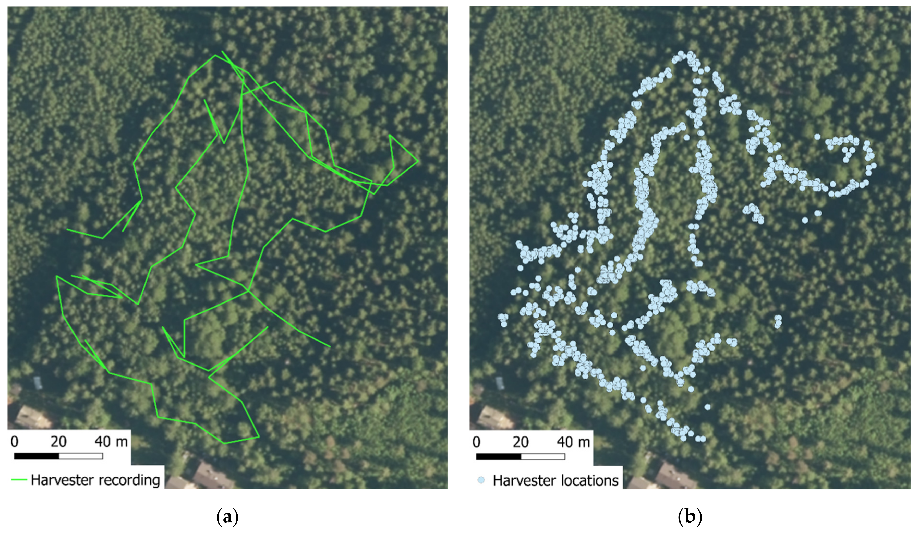
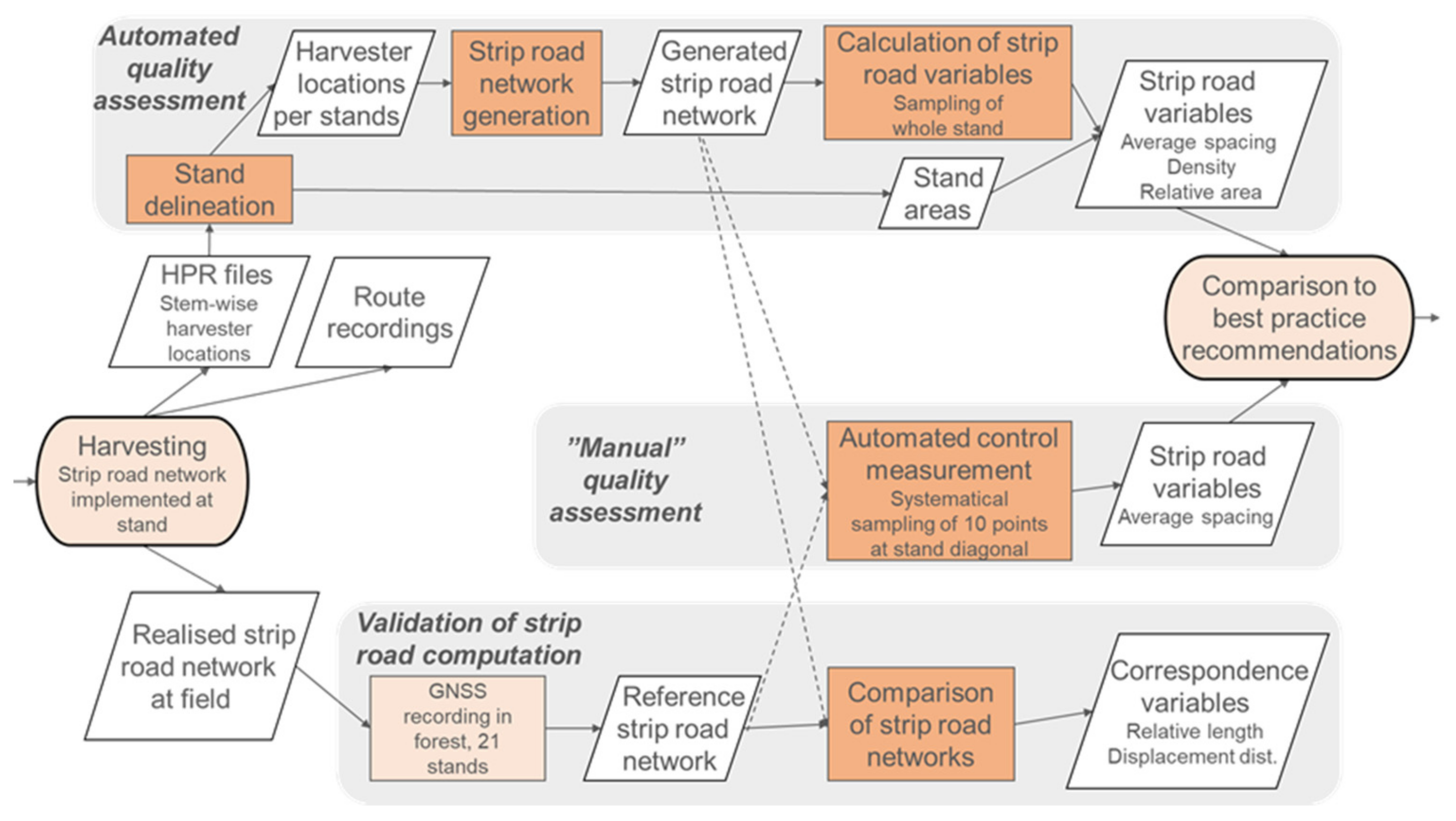
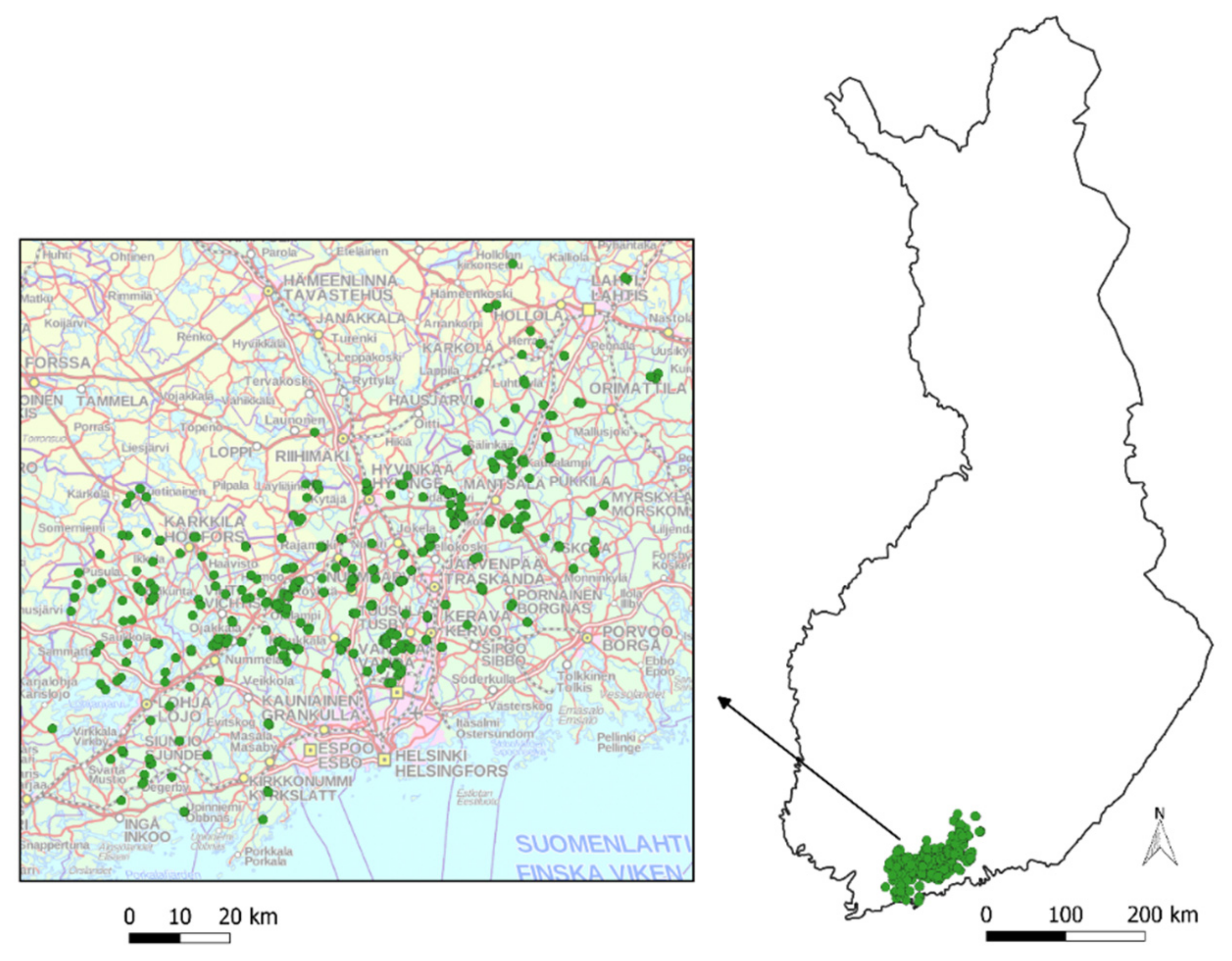
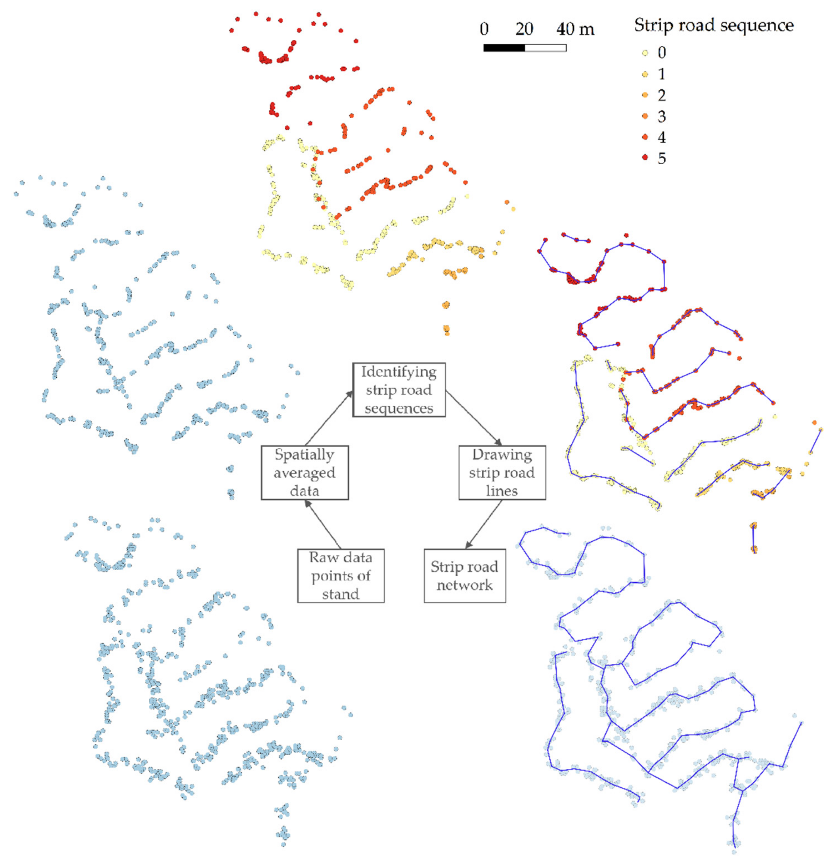
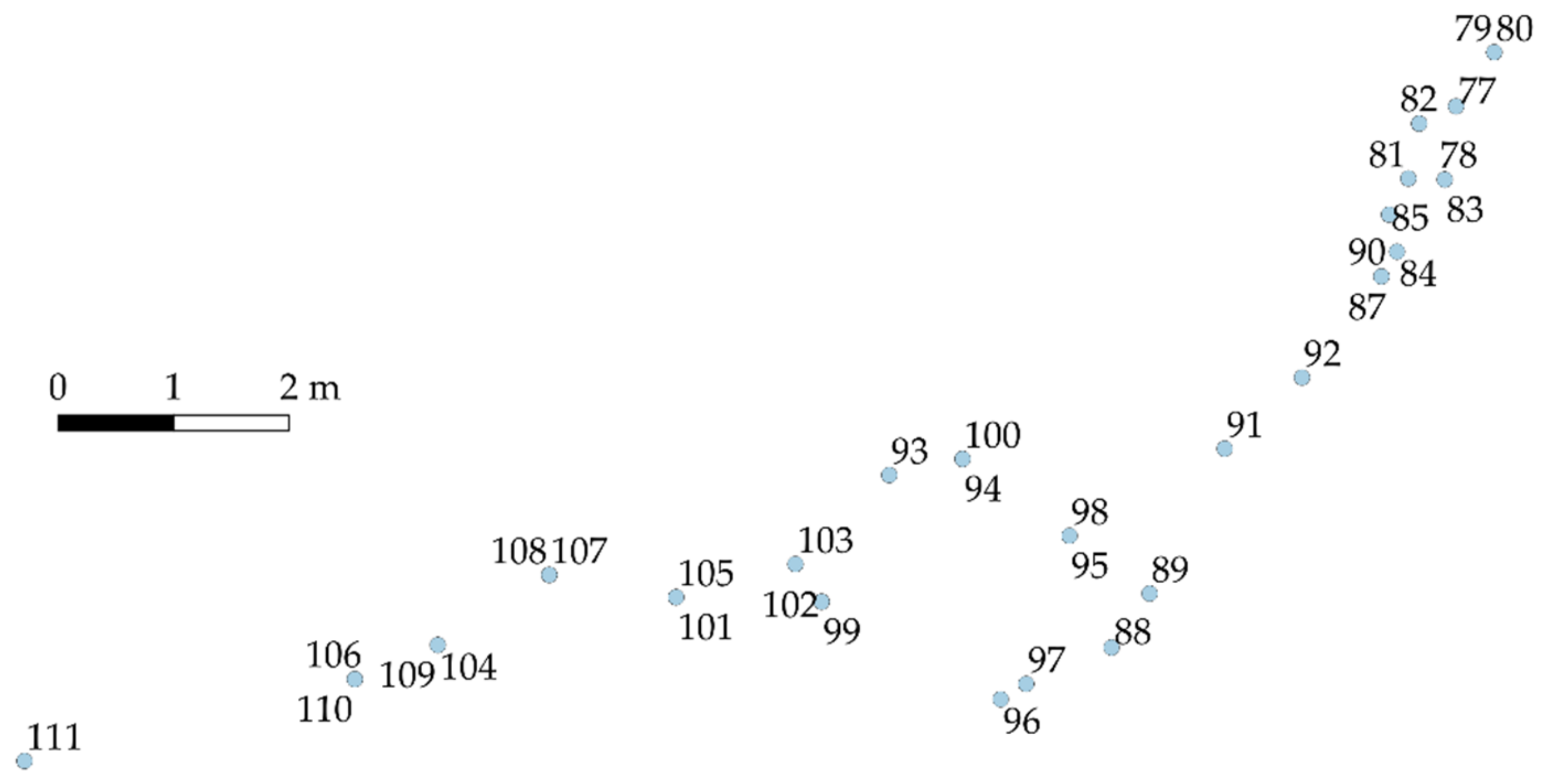
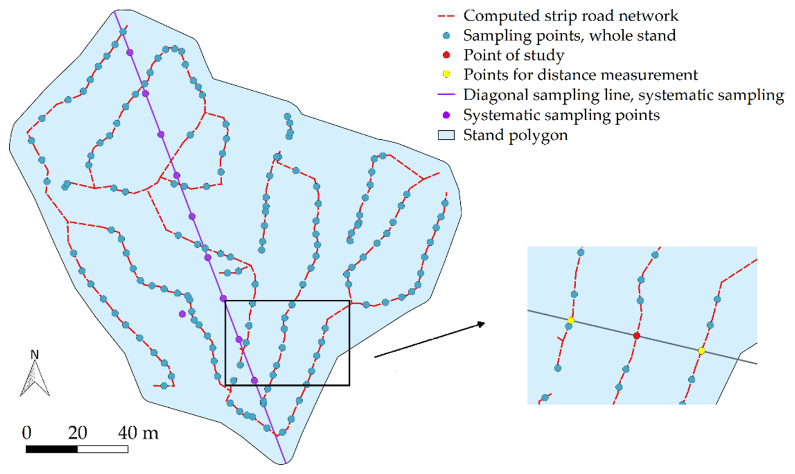
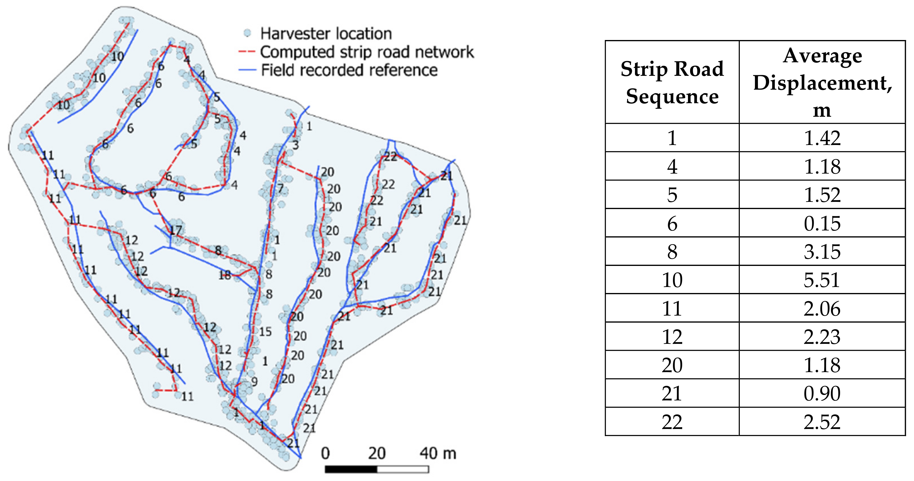
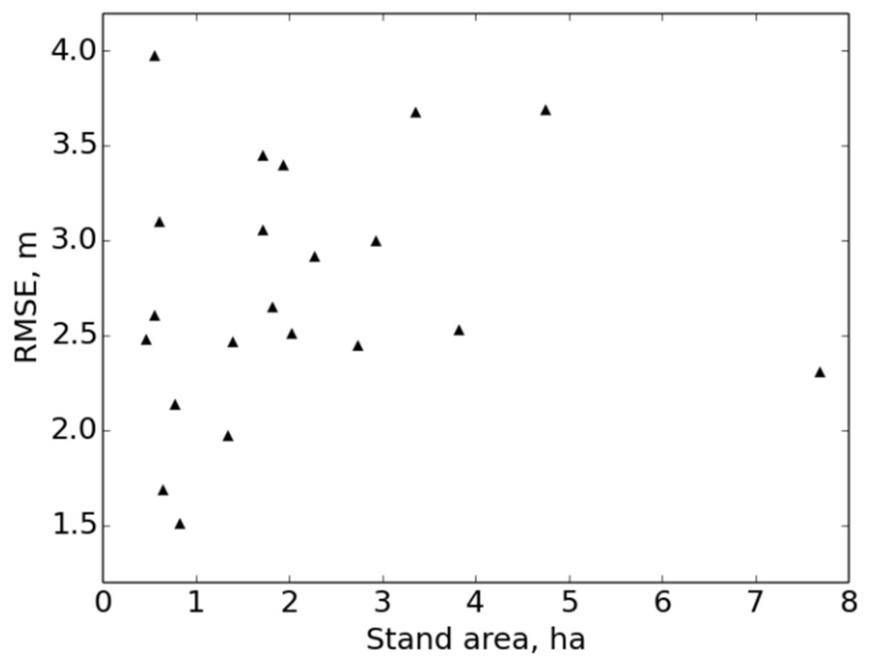
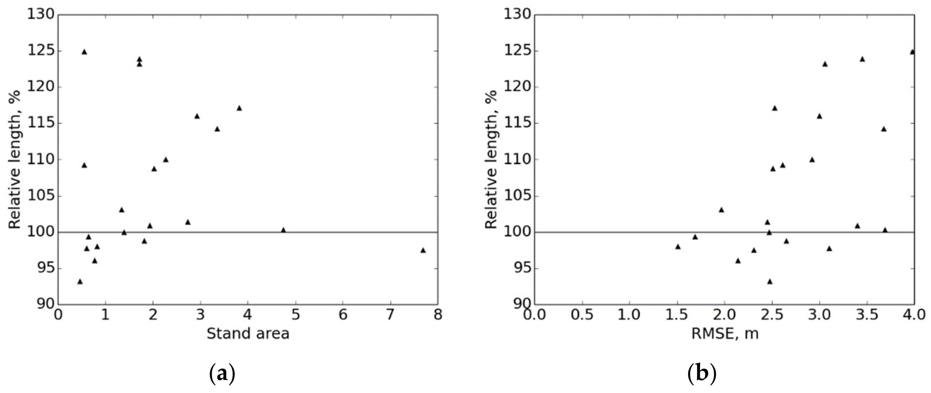
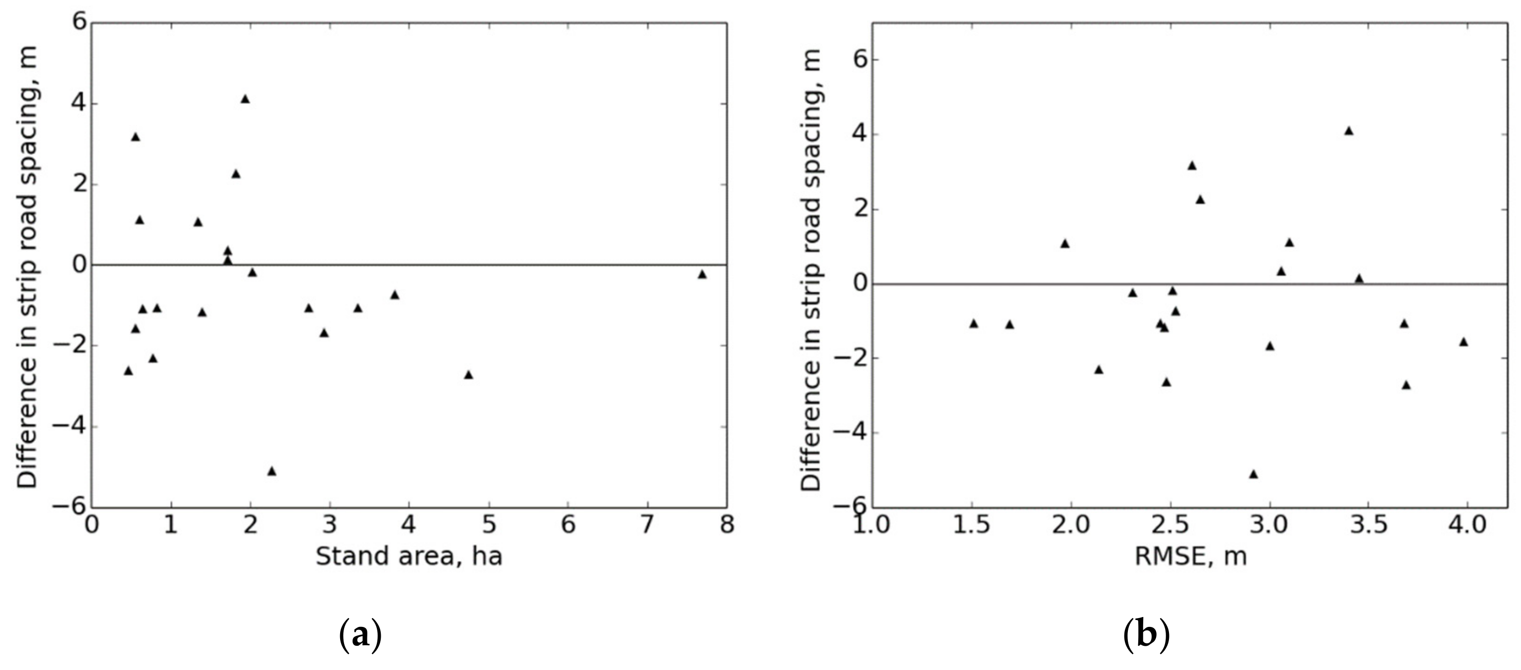
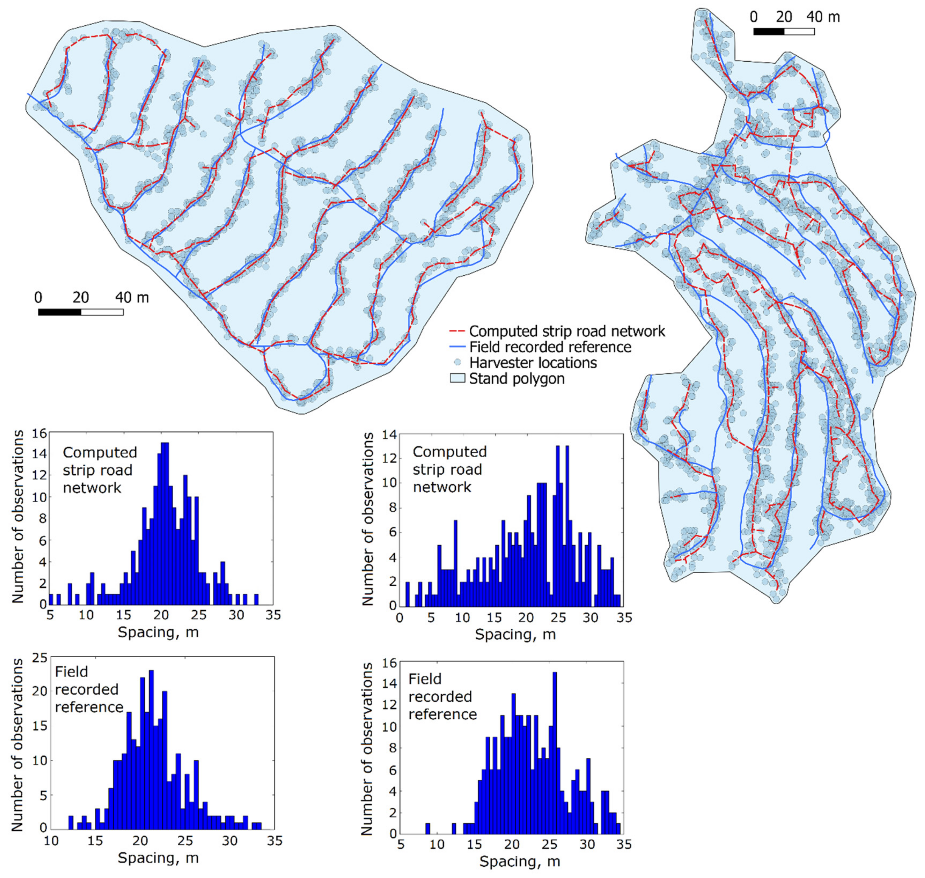
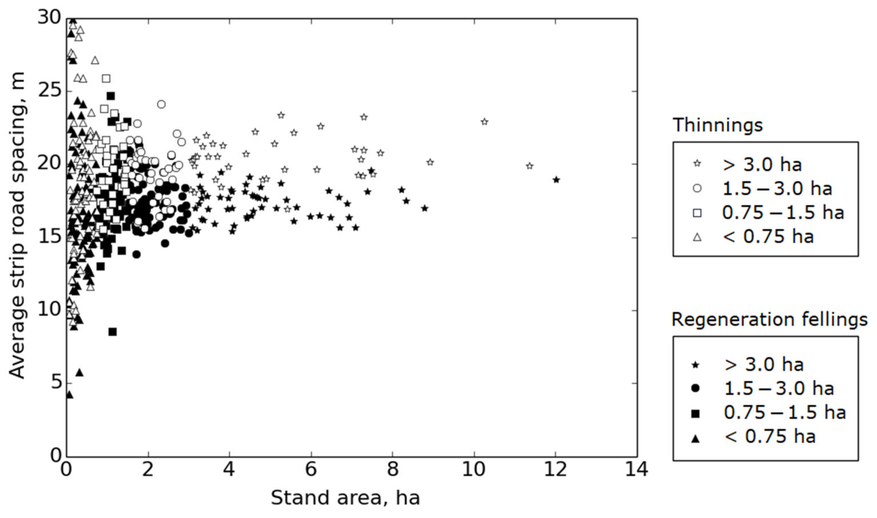
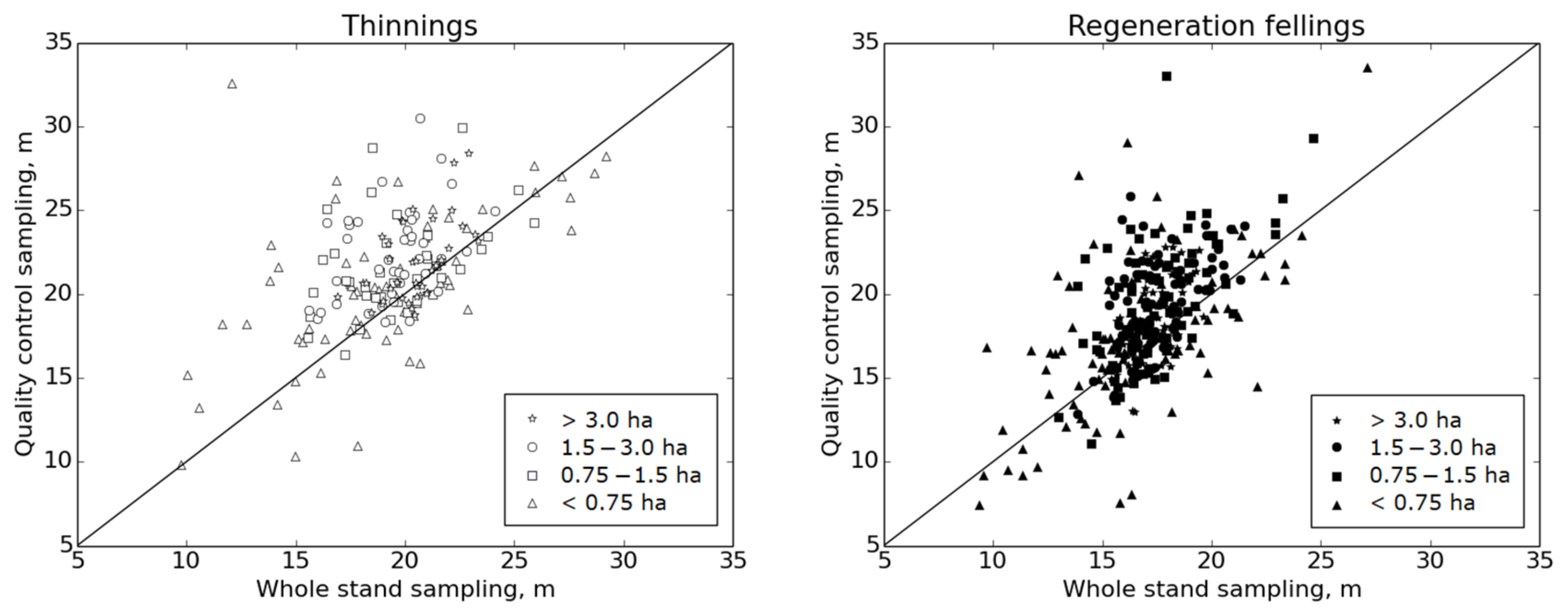
Table 1.
The number of automatically delineated stands in this study by harvesting method and stand area class.
Table 1.
The number of automatically delineated stands in this study by harvesting method and stand area class.
| Harvesting Method | Number of Stands | ||||
|---|---|---|---|---|---|
| <0.75 ha | 0.75–1.5 ha | 1.5–3 ha | >3 ha | Total | |
| First thinning | 18 | 8 | 11 | 5 | 42 |
| Later thinning | 59 | 29 | 29 | 35 | 152 |
| Clear cutting | 104 | 66 | 74 | 49 | 293 |
| Seed tree or shelter tree cutting | 21 | 18 | 10 | 8 | 57 |
| Total | 202 | 121 | 124 | 97 | 544 |
Table 2.
Detailed strip road variables of the reference dataset. The number of sampling points refers to the comparison of the strip road network geometries. Note that, for the reference strip road networks, the average spacing is also sampled using the systematic quality control measurement method, in addition to sampling the whole stand. The strip road route recordings by harvester were available only for five stands; therefore, some of the values of the “Strip road length recorded by harvester, m” column are left empty.
| StandID | Stand Area, ha | Strip Road Length, m | Relative Length, % | Number of Sampling Points | RMSE of Displacement Distances, m | Average Spacing of Strip Road, m | Strip Road per Stand Area, m/ha | |||||
|---|---|---|---|---|---|---|---|---|---|---|---|---|
| Computed | Reference | Recorded by Harvester (% of Reference) | Per Stand | Per 100 m Reference | Whole Stand Sampling | Reference with Systematic 10-Point Sampling | ||||||
| Computed | Reference | |||||||||||
| 1_2 | 0.82 | 444 | 453 | 780 (172%) | 98.0 | 86 | 19.0 | 1.51 | 20.5 | 21.5 | 21.5 | 541.5 |
| 1_1 | 0.65 | 347 | 349 | 562 (161%) | 99.4 | 69 | 19.8 | 1.69 | 20.7 | 21.8 | 22.8 | 533.8 |
| 231_1 | 1.34 | 742 | 720 | 938 (130%) | 103.1 | 141 | 19.6 | 1.97 | 21.8 | 20.8 | 19.1 | 553.7 |
| 23_1 | 0.78 | 448 | 466 | 96.1 | 78 | 16.7 | 2.14 | 17.7 | 20 | 18.6 | 574.4 | |
| 400_1 | 7.69 | 4446 | 4560 | 97.5 | 857 | 18.8 | 2.31 | 19.3 | 19.6 | 20.0 | 578.2 | |
| 252_1 | 2.74 | 1623 | 1601 | 101.4 | 367 | 22.9 | 2.45 | 20.6 | 21.7 | 21.4 | 592.3 | |
| 337_1 | 1.39 | 840 | 840 | 100.0 | 143 | 17.0 | 2.47 | 21.2 | 22.4 | 19.6 | 604.3 | |
| 20_1 | 0.47 | 259 | 278 | 93.2 | 67 | 24.1 | 2.48 | 17.5 | 20.1 | 24.4 | 551.1 | |
| 361_1 | 2.03 | 1283 | 1179 | 108.8 | 233 | 19.8 | 2.51 | 19.1 | 19.3 | 16.7 | 632.0 | |
| 370_11 | 3.82 | 2352 | 2009 | 117.1 | 428 | 21.3 | 2.53 | 19.1 | 19.8 | 18.9 | 615.7 | |
| 83_1 | 0.56 | 342 | 313 | 1274 (407%) | 109.3 | 73 | 23.3 | 2.61 | 21.6 | 18.4 | 17.9 | 610.7 |
| 168_2 | 1.82 | 1099 | 1112 | 98.8 | 213 | 19.2 | 2.65 | 19.4 | 17.1 | 19.6 | 603.8 | |
| 326_1 | 2.27 | 1414 | 1285 | 110.0 | 258 | 20.1 | 2.92 | 16.9 | 22 | 23.2 | 622.9 | |
| 310_1 | 2.93 | 1976 | 1703 | 3405 (200%) | 116.0 | 444 | 26.1 | 3.00 | 18.8 | 20.5 | 18.8 | 674.4 |
| 370_12 | 1.72 | 1087 | 882 | 123.2 | 185 | 21.0 | 3.06 | 19.4 | 19 | 20.4 | 632.0 | |
| 30_1 | 0.61 | 357 | 365 | 97.8 | 54 | 14.8 | 3.10 | 23.5 | 22.4 | 22.8 | 585.2 | |
| 375_1 | 1.93 | 1159 | 1149 | 100.9 | 235 | 20.5 | 3.40 | 22.4 | 18.3 | 17.9 | 600.5 | |
| 384_1 | 1.71 | 1068 | 862 | 123.9 | 174 | 20.2 | 3.45 | 20.4 | 20.3 | 23.3 | 624.6 | |
| 401_1 | 3.35 | 2119 | 1854 | 114.3 | 404 | 21.8 | 3.68 | 18.2 | 19.3 | 18.1 | 632.5 | |
| 61_1 | 4.75 | 2381 | 2374 | 100.3 | 454 | 19.1 | 3.69 | 20.2 | 22.9 | 24.0 | 501.3 | |
| 405_5 | 0.55 | 421 | 337 | 124.9 | 103 | 30.6 | 3.98 | 14.4 | 15.9 | 20.1 | 765.5 | |
| Average | 2.1 | 1212 | 1143 | 106.5 | 235 | 20.8 | 2.7 | 19.7 | 20.2 | 20.4 | 601 | |
Table 3.
Average strip road variables by stand area class and harvesting method. The standard deviations are provided in parentheses, and in this table, they describe the variation of the stand-wise values of the variable within each area class.
Table 3.
Average strip road variables by stand area class and harvesting method. The standard deviations are provided in parentheses, and in this table, they describe the variation of the stand-wise values of the variable within each area class.
| Harvesting Method | Area Class, ha | Number of Stands 1 | Strip Road Density, m/ha | Whole Stand Sampling | Systematic Sampling of Quality Control | Relative Area of Strip Road Network, % | ||
|---|---|---|---|---|---|---|---|---|
| Average Spacing, m | Sample Number Average 2 | Average Spacing, m | Sample Number Average 2 | |||||
| First thinning | <0.75 | 17 (16) | 618 (85) | 18.1 (3.4) | 23 (15) | 20.0 (3.5) | 6.9 (2.6) | 27.8 (3.6) |
| 0.75–1.5 | 8 | 587 (35) | 19.2 (1.6) | 76 (11) | 21.1 (2.1) | 8.8 (1.9) | 26.3 (1.5) | |
| 1.5–3 | 11 | 627 (49) | 18.5 (1.8) | 135 (23) | 21.7 (2.3) | 8.6 (1.9) | 27.6 (2.0) | |
| >3 | 5 | 604 (20) | 19.5 (0.8) | 379 (142) | 20.3 (0.4) | 10 (0.0) | 26.8 (0.7) | |
| Later thinning | <0.75 | 52 (47) | 562 (89) | 18.9 (5.1) | 17 (13) | 20.6 (4.8) | 4.9 (2.7) | 25.5 (3.7) |
| 0.75–1.5 | 29 | 546 (72) | 19.7 (2.8) | 67 (30) | 21.8 (3.1) | 8.1 (2.7) | 24.4 (2.9) | |
| 1.5–3 | 29 | 543 (77) | 19.8 (1.8) | 117 (46) | 22.6 (2.9) | 9.0 (1.6) | 24.2 (3.3) | |
| >3 | 35 | 561 (60) | 20.6 (1.4) | 291 (124) | 22.0 (2.4) | 9.6 (1.1) | 24.9 (2.5) | |
| Clear cutting | <0.75 | 91 (77) | 655 (111) | 16.1 (3.8) | 22 (17) | 17.1 (4.7) | 5.5 (2.8) | 29.5 (4.6) |
| 0.75–1.5 | 66 | 671 (88) | 17.1 (1.7) | 79 (24) | 18.9 (3.2) | 8.2 (2.3) | 29.7 (3.8) | |
| 1.5–3 | 74 | 650 (72) | 17.3 (1.4) | 148 (53) | 19.0 (2.8) | 8.8 (2.0) | 28.8 (3.1) | |
| >3 | 49 | 683 (58) | 17.2 (1.1) | 391 (146) | 18.1 (2.3) | 9.8 (0.7) | 30.1 (2.5) | |
| Seed tree or shelter tree cutting | <0.75 | 15 (10) | 521 (108) | 18.9 (6.3) | 15 (12) | 19.7 (4.4) | 5.6 (3.1) | 23.9 (4.7) |
| 0.75–1.5 | 18 (16) | 545 (188) | 18.3 (3.5) | 54 (29) | 21.1 (4.9) | 6.8 (3.5) | 24.3 (8.1) | |
| 1.5–3 | 10 | 609 (105) | 18.9 (2.0) | 135 (64) | 20.5 (2.2) | 8.5 (2.6) | 27.0 (4.6) | |
| >3 | 8 | 673 (44) | 18.0 (0.8) | 344 (93) | 20.2 (1.6) | 9.3 (2.0) | 29.8 (1.8) | |
1 The number of stands from which the systematical sampling of strip road spacing could be performed automatically is in parentheses if it differs from the number of stands in the area category. 2 Note that the standard deviation of the number of sampling points is calculated using an assumption of normal distribution, although the maximum number of samples is 10.
Publisher’s Note: MDPI stays neutral with regard to jurisdictional claims in published maps and institutional affiliations. |
© 2022 by the authors. Licensee MDPI, Basel, Switzerland. This article is an open access article distributed under the terms and conditions of the Creative Commons Attribution (CC BY) license (https://creativecommons.org/licenses/by/4.0/).
Share and Cite
MDPI and ACS Style
Ovaskainen, H.; Riekki, K. Computation of Strip Road Networks Based on Harvester Location Data. Forests 2022, 13, 782. https://0-doi-org.brum.beds.ac.uk/10.3390/f13050782
AMA Style
Ovaskainen H, Riekki K. Computation of Strip Road Networks Based on Harvester Location Data. Forests. 2022; 13(5):782. https://0-doi-org.brum.beds.ac.uk/10.3390/f13050782
Chicago/Turabian StyleOvaskainen, Heikki, and Kirsi Riekki. 2022. "Computation of Strip Road Networks Based on Harvester Location Data" Forests 13, no. 5: 782. https://0-doi-org.brum.beds.ac.uk/10.3390/f13050782
Note that from the first issue of 2016, this journal uses article numbers instead of page numbers. See further details here.