
Modeling of Hydrogen Production by Applying Biomass Gasification: Artificial Neural Network Modeling Approach


 and
and
Abstract
:1. Introduction
2. Material and Methods
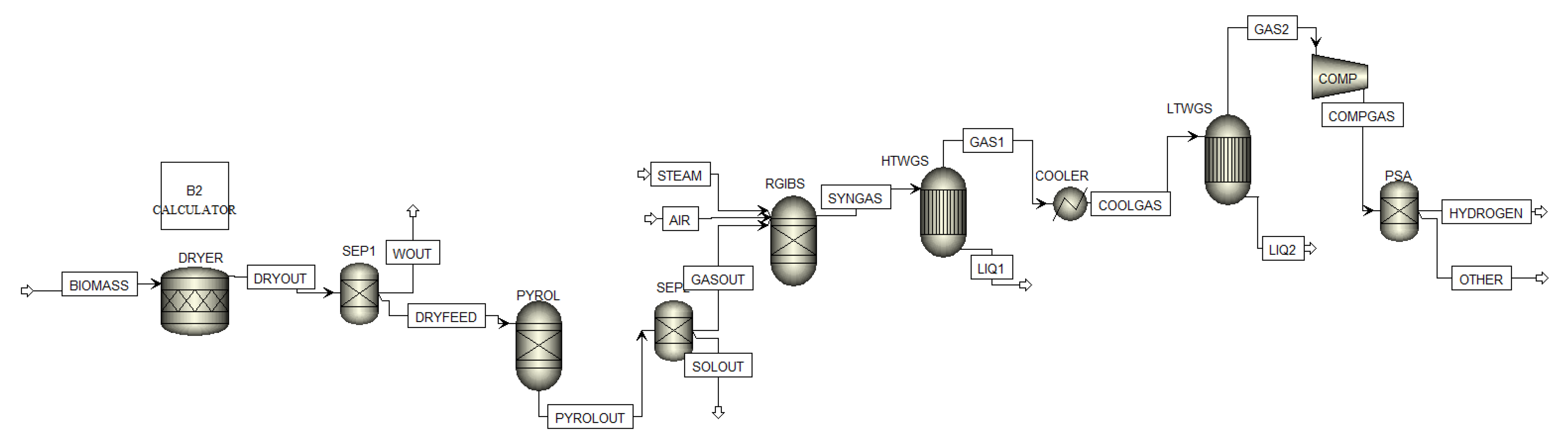
2.1. Method of Simulation
2.1.1. Gasification Module
2.1.2. Water–Gas Shift Module
2.1.3. Separation Unit Module
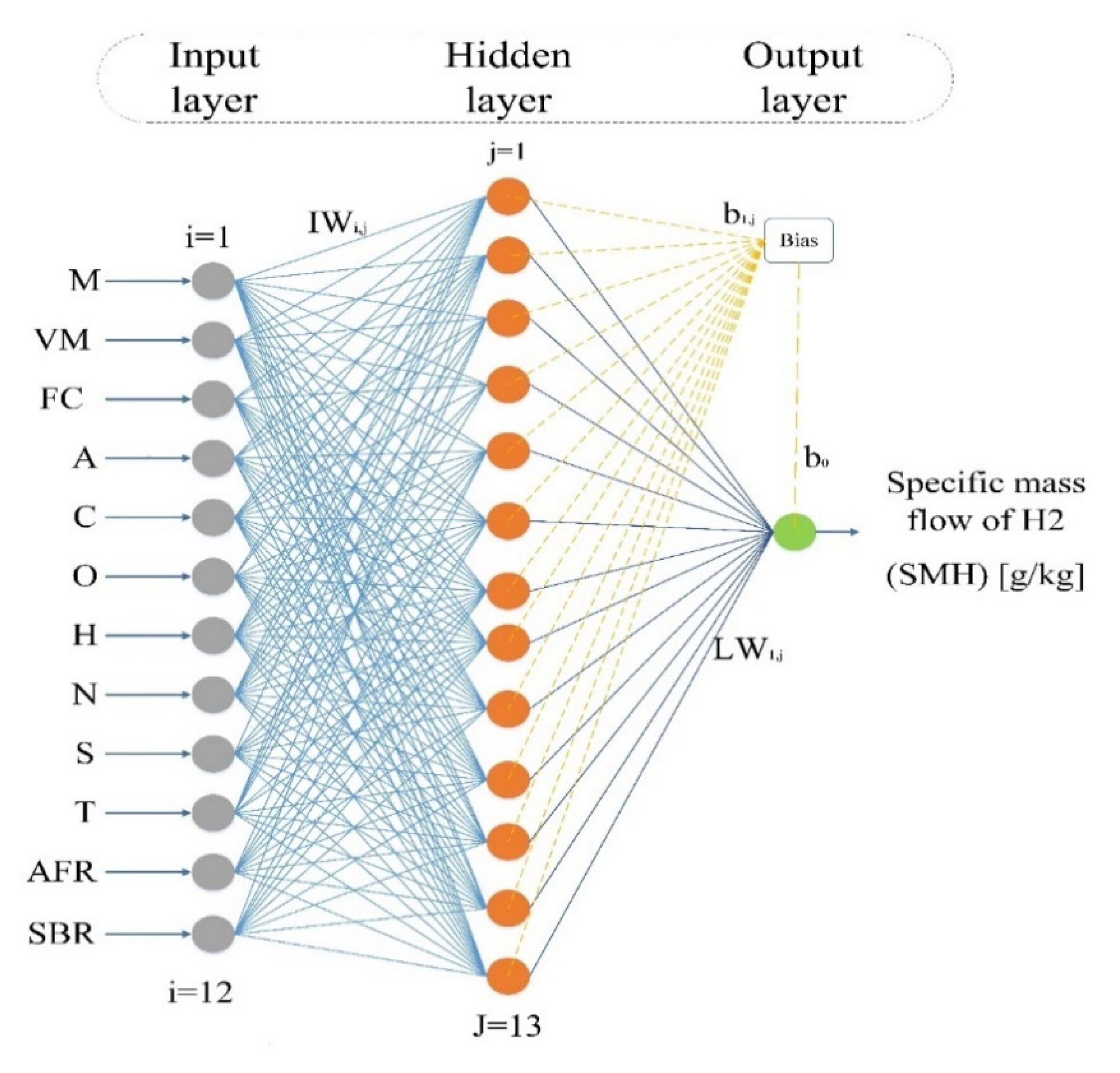
2.2. Concept of the Developed ANN Model
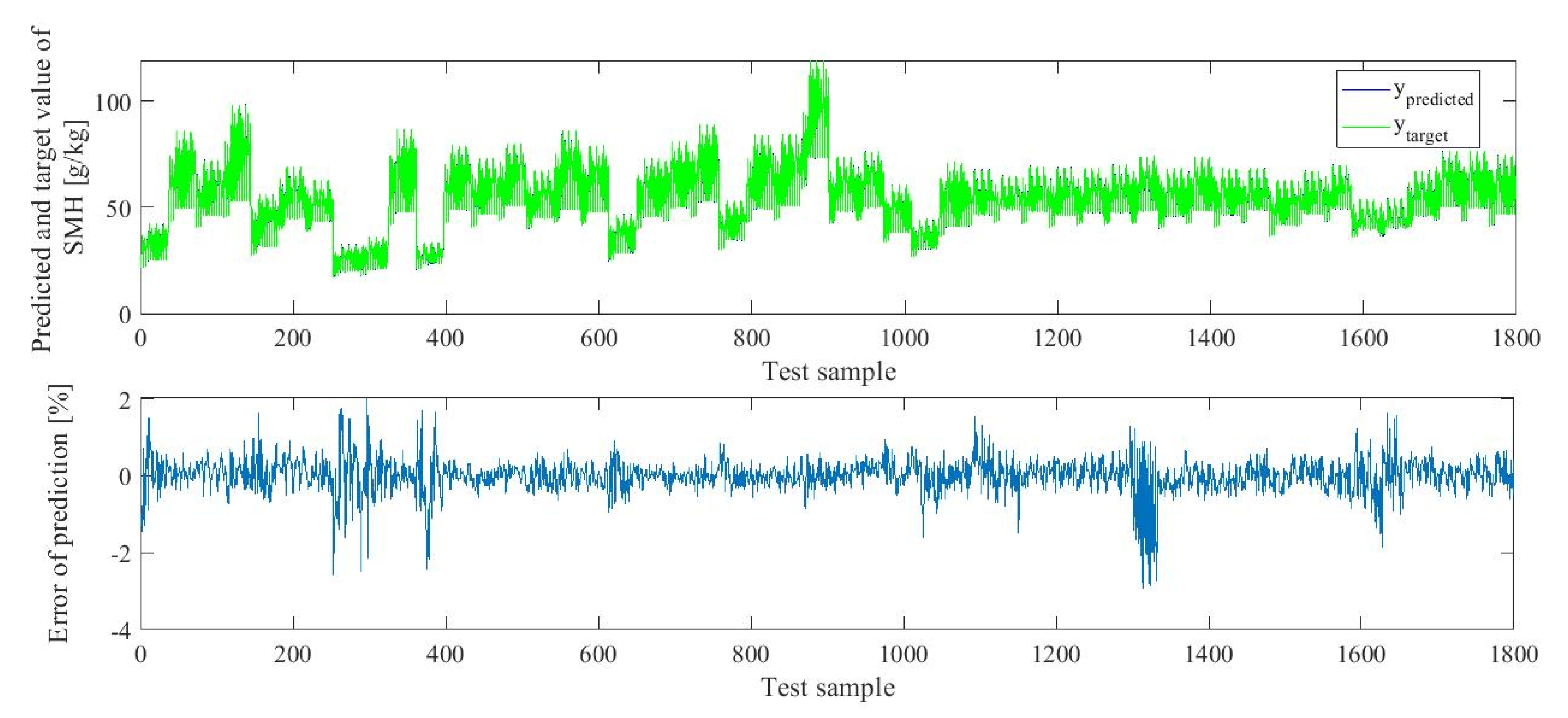
2.3. Training and Testing of the ANN-Based Model
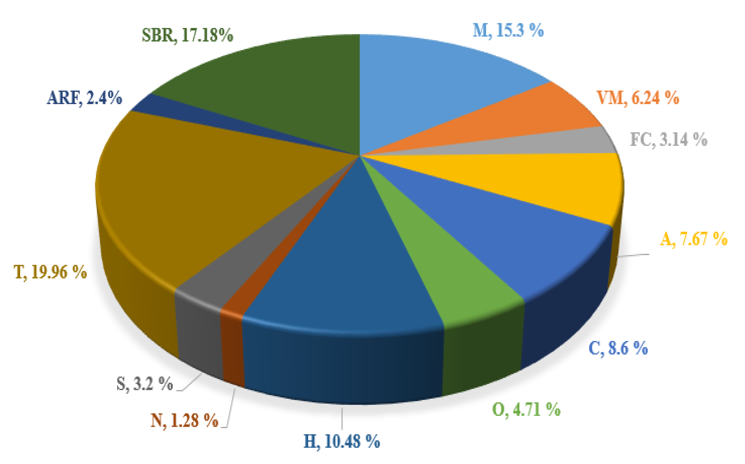
2.4. Calculation of Relative Impact of Inputs on the Output
3. Results and Discussion
4. Conclusions
Author Contributions
Funding
Institutional Review Board Statement
Informed Consent Statement
Data Availability Statement
Conflicts of Interest
References
- Safarian, S.; Khodaparast, P.; Kateb, M. Modeling and technical-economic optimization of electricity supply network by three photovoltaic systems. J. Sol. Energy Eng. 2014, 136, 024501. [Google Scholar] [CrossRef]
- Rajaeifar, M.A.; Akram, A.; Ghobadian, B.; Rafiee, S.; Heijungs, R.; Tabatabaei, M. Environmental impact assessment of olive pomace oil biodiesel production and consumption: A comparative lifecycle assessment. Energy 2016, 106, 87–102. [Google Scholar] [CrossRef]
- Talebnia, F.; Karakashev, D.; Angelidaki, I. Production of bioethanol from wheat straw: An overview on pretreatment, hydrolysis and fermentation. Bioresour. Technol. 2010, 101, 4744–4753. [Google Scholar] [CrossRef]
- Safarian, S.; Unnthorsson, R.; Richter, C. Techno-economic analysis of power production by using waste biomass gasification. J. Power Energy Eng. 2020, 8, 1–8. [Google Scholar] [CrossRef]
- Zeng, J.; Xiao, R.; Zhang, H.; Wang, Y.; Zeng, D.; Ma, Z. Chemical looping pyrolysis-gasification of biomass for high h2/co syngas production. Fuel Process. Technol. 2017, 168, 116–122. [Google Scholar] [CrossRef]
- Luo, H.; Lin, W.; Song, W.; Li, S.; Dam-Johansen, K.; Wu, H. Three dimensional full-loop cfd simulation of hydrodynamics in a pilot-scale dual fluidized bed system for biomass gasification. Fuel Process. Technol. 2019, 195, 106146. [Google Scholar] [CrossRef]
- Kumar, B.; Bhardwaj, N.; Agrawal, K.; Chaturvedi, V.; Verma, P. Current perspective on pretreatment technologies using lignocellulosic biomass: An emerging biorefinery concept. Fuel Process. Technol. 2020, 199, 106244. [Google Scholar] [CrossRef]
- Safarian, S.; Sattari, S.; Hamidzadeh, Z. Sustainability assessment of biodiesel supply chain from various biomasses and conversion technologies. Biophys. Econ. Resour. Qual. 2018, 3, 6. [Google Scholar] [CrossRef]
- Safarian, S.; Sattari, S.; Unnthorsson, R.; Hamidzadeh, Z. Prioritization of bioethanol production systems from agricultural and waste agricultural biomass using multi-criteria decision making. Biophys. Econ. Resour. Qual. 2019, 4, 4. [Google Scholar] [CrossRef]
- Safarian, S.; Unnthorsson, R. An assessment of the sustainability of lignocellulosic bioethanol production from wastes in iceland. Energies 2018, 11, 1493. [Google Scholar] [CrossRef] [Green Version]
- Nguyen, T.L.T.; Hermansen, J.E.; Nielsen, R.G. Environmental assessment of gasification technology for biomass conversion to energy in comparison with other alternatives: The case of wheat straw. J. Clean. Prod. 2013, 53, 138–148. [Google Scholar] [CrossRef]
- Huda, A.; Mekhilef, S.; Ahsan, A. Biomass energy in bangladesh: Current status and prospects. Renew. Sustain. Energy Rev. 2014, 30, 504–517. [Google Scholar] [CrossRef]
- Safarian, S.; Unnþórsson, R.; Richter, C. A review of biomass gasification modelling. Renew. Sustain. Energy Rev. 2019, 110, 378–391. [Google Scholar] [CrossRef]
- Inayat, A.; Raza, M.; Khan, Z.; Ghenai, C.; Aslam, M.; Shahbaz, M.; Ayoub, M. Flowsheet modeling and simulation of biomass steam gasification for hydrogen production. Chem. Eng. Technol. 2020, 43, 649–660. [Google Scholar] [CrossRef]
- Safarian, S.; Saryazdi, S.M.E.; Unnthorsson, R.; Richter, C. Artificial neural network integrated with thermodynamic equilibrium modeling of downdraft biomass gasification-power production plant. Energy 2020, 213, 118800. [Google Scholar] [CrossRef]
- Safarian, S.; Unnthorsson, R.; Richter, C. The equivalence of stoichiometric and non-stoichiometric methods for modeling gasification and other reaction equilibria. Renew. Sustain. Energy Rev. 2020, 131, 109982. [Google Scholar] [CrossRef]
- All Power Laboratories. Available online: http://www.allpowerlabs.com/ (accessed on 12 December 2019).
- Safarian, S.; Unnthorsson, R.; Richter, C. Simulation and performance analysis of integrated gasification–syngas fermentation plant for lignocellulosic ethanol production. Fermentation 2020, 6, 68. [Google Scholar] [CrossRef]
- Marcantonio, V.; De Falco, M.; Capocelli, M.; Bocci, E.; Colantoni, A.; Villarini, M. Process analysis of hydrogen production from biomass gasification in fluidized bed reactor with different separation systems. Int. J. Hydrog. Energy 2019, 44, 10350–10360. [Google Scholar] [CrossRef]
- Safarian, S.; Unnthorsson, R.; Richter, C. Gasification of Woody Biomasses and Forestry Residues: Simulation, Performance Analysis, and Environmental Impact. Energy 2020, 197, 117268. [Google Scholar] [CrossRef]
- Balat, H.; Kırtay, E. Hydrogen from biomass–present scenario and future prospects. Int. J. Hydrog. Energy 2010, 35, 7416–7426. [Google Scholar] [CrossRef]
- Martin, M.; Svensson, N.; Fonseca, J.; Eklund, M. Quantifying the environmental performance of integrated bioethanol and biogas production. Renew. Energy 2014, 61, 109–116. [Google Scholar] [CrossRef]
- Yoon, S.J.; Son, Y.-I.; Kim, Y.-K.; Lee, J.-G. Gasification and power generation characteristics of rice husk and rice husk pellet using a downdraft fixed-bed gasifier. Renew. Energy 2012, 42, 163–167. [Google Scholar] [CrossRef]
- Safarian, S.; Saboohi, Y.; Kateb, M. Evaluation of energy recovery and potential of hydrogen production in iranian natural gas transmission network. Energy Policy 2013, 61, 65–77. [Google Scholar] [CrossRef]
- Çağlar, A.; Demirbaş, A. Hydrogen rich gas mixture from olive husk via pyrolysis. Energy Convers. Manag. 2002, 43, 109–117. [Google Scholar] [CrossRef]
- Frigo, S.; Spazzafumo, G. Cogeneration of power and substitute of natural gas using biomass and electrolytic hydrogen. Int. J. Hydrog. Energy 2018, 43, 11696–11705. [Google Scholar] [CrossRef]
- Li, Q.; Song, G.; Xiao, J.; Sun, T.; Yang, K. Exergy analysis of biomass staged-gasification for hydrogen-rich syngas. Int. J. Hydrog. Energy 2019, 44, 2569–2579. [Google Scholar] [CrossRef]
- Safarian, S.; Richter, C.; Unnthorsson, R. Waste biomass gasification simulation using aspen plus: Performance evaluation of wood chips, sawdust and mixed paper wastes. J. Power Energy Eng. 2019, 7, 12–30. [Google Scholar] [CrossRef] [Green Version]
- Safarian, S.; Unnthorsson, R.; Richter, C. Performance analysis and environmental assessment of small-scale waste biomass gasification integrated chp in iceland. Fermentation 2020, 7, 61. [Google Scholar] [CrossRef]
- Safarian, S.; Unnthorsson, R.; Richter, C. Simulation of small-scale waste biomass gasification integrated power production: A comparative performance analysis for timber and wood waste. Int. J. Appl. Power Eng. IJAPE 2020, 9, 147–152. [Google Scholar] [CrossRef]
- Safarian, S.; Unnthorsson, R.; Richter, C. Techno-economic and environmental assessment of power supply chain by using waste biomass gasification in iceland. Biophys. Econ. Sustain. 2020, 5, 7. [Google Scholar] [CrossRef]
- Damartzis, T.; Michailos, S.; Zabaniotou, A. Energetic assessment of a combined heat and power integrated biomass gasification–internal combustion engine system by using aspen plus®. Fuel Process. Technol. 2012, 95, 37–44. [Google Scholar] [CrossRef]
- Kobayashi, N.; Tanaka, M.; Piao, G.; Kobayashi, J.; Hatano, S.; Itaya, Y.; Mori, S. High temperature air-blown woody biomass gasification model for the estimation of an entrained down-flow gasifier. Waste Manag. 2009, 29, 245–251. [Google Scholar] [CrossRef]
- Porcu, A.; Sollai, S.; Marotto, D.; Mureddu, M.; Ferrara, F.; Pettinau, A. Techno-economic analysis of a small-scale biomass-to-energy bfb gasification-based system. Energies 2019, 12, 494. [Google Scholar] [CrossRef] [Green Version]
- Roy, D.; Samanta, S.; Ghosh, S. Thermo-economic assessment of biomass gasification-based power generation system consists of solid oxide fuel cell, supercritical carbon dioxide cycle and indirectly heated air turbine. Clean Technol. Environ. Policy 2019, 21, 827–845. [Google Scholar] [CrossRef]
- Safarianbana, S.; Unnthorsson, R.; Richter, C. Development of a new stoichiometric equilibrium-based model for wood chips and mixed paper wastes gasification by aspen plus. In ASME International Mechanical Engineering Congress and Exposition; American Society of Mechanical Engineers: Salt Lake City, UT, USA, 2019; p. V006T006A00. [Google Scholar]
- Shayan, E.; Zare, V.; Mirzaee, I. Hydrogen production from biomass gasification; a theoretical comparison of using different gasification agents. Energy Convers. Manag. 2018, 159, 30–41. [Google Scholar] [CrossRef]
- Gil, J.; Corella, J.; Aznar, M.A.P.; Caballero, M.A. Biomass gasification in atmospheric and bubbling fluidized bed: Effect of the type of gasifying agent on the product distribution. Biomass Bioenergy 1999, 17, 389–403. [Google Scholar] [CrossRef]
- George, J.; Arun, P.; Muraleedharan, C. Assessment of producer gas composition in air gasification of biomass using artificial neural network model. Int. J. Hydrog. Energy 2018, 43, 9558–9568. [Google Scholar] [CrossRef]
- Nasir, V.; Nourian, S.; Avramidis, S.; Cool, J. Classification of thermally treated wood using machine learning techniques. Wood Sci. Technol. 2019, 53, 275–288. [Google Scholar] [CrossRef]
- Nasir, V.; Nourian, S.; Avramidis, S.; Cool, J. Prediction of physical and mechanical properties of thermally modified wood based on color change evaluated by means of “group method of data handling” (gmdh) neural network. Holzforschung 2019, 73, 381–392. [Google Scholar] [CrossRef]
- Rostampour, V.; Motlagh, A.M.; Komarizadeh, M.H.; Sadeghi, M.; Bernousi, I.; Ghanbari, T. Using artificial neural network (ann) technique for prediction of apple bruise damage. Aust. J. Crop Sci. 2013, 7, 1442–1448. [Google Scholar]
- Capizzi, G.; Sciuto, G.L.; Napoli, C.; Woźniak, M.; Susi, G. A spiking neural network-based long-term prediction system for biogas production. Neural Netw. 2020, 129, 271–279. [Google Scholar] [CrossRef] [PubMed]
- Baruah, D.; Baruah, D.; Hazarika, M. Artificial neural network based modeling of biomass gasification in fixed bed downdraft gasifiers. Biomass Bioenergy 2017, 98, 264–271. [Google Scholar] [CrossRef]
- Puig-Arnavat, M.; Hernández, J.A.; Bruno, J.C.; Coronas, A. Artificial neural network models for biomass gasification in fluidized bed gasifiers. Biomass Bioenergy 2013, 49, 279–289. [Google Scholar] [CrossRef]
- Schmidt, A.; Creason, W.; Law, B.E. Estimating regional effects of climate change and altered land use on biosphere carbon fluxes using distributed time delay neural networks with bayesian regularized learning. Neural Netw. 2018, 108, 97–113. [Google Scholar] [CrossRef] [PubMed]
- Safarian, S.; Saryazdi, S.M.E.; Unnthorsson, R.; Richter, C. Artificial neural network modeling of bioethanol production via syngas fermentation. Biophys. Econ. Sustain. 2021, 6, 1–13. [Google Scholar] [CrossRef]
- Safarian, S.; Bararzadeh, M. Exergy analysis of high-performance cycles for gas turbine with air-bottoming. J. Mech. Eng. Res. 2012, 5, 38–49. [Google Scholar]
- Safarian, S.; Unnthorsson, R.; Richter, C. Performance analysis of power generation by wood and woody biomass gasification in a downdraft gasifier. J. Appl. Power Eng. 2021, 10, 80–88. [Google Scholar]
- Vassilev, S.V.; Baxter, D.; Andersen, L.K.; Vassileva, C.G. An overview of the chemical composition of biomass. Fuel 2010, 89, 913–933. [Google Scholar] [CrossRef]
- Miles, T.; Baxter, L.; Bryers, R.; Jenkins, B.; Oden, L. Alkali deposits found in biomass power plants: A preliminary investigation of their extent and nature. Alkalis Altern. Fuels 1995. [Google Scholar] [CrossRef] [Green Version]
- Bryers, R.W. Fireside slagging, fouling, and high-temperature corrosion of heat-transfer surface due to impurities in steam-raising fuels. Prog. Energy Combust. Sci. 1996, 22, 29–120. [Google Scholar] [CrossRef]
- Theis, M.; Skrifvars, B.-J.; Hupa, M.; Tran, H. Fouling tendency of ash resulting from burning mixtures of biofuels. Part 1: Deposition rates. Fuel 2006, 85, 1125–1130. [Google Scholar] [CrossRef]
- Theis, M.; Skrifvars, B.-J.; Zevenhoven, M.; Hupa, M.; Tran, H. Fouling tendency of ash resulting from burning mixtures of biofuels. Part 2: Deposit chemistry. Fuel 2006, 85, 1992–2001. [Google Scholar] [CrossRef]
- Zevenhoven-Onderwater, M.; Backman, R.; Skrifvars, B.-J.; Hupa, M. The ash chemistry in fluidised bed gasification of biomass fuels. Part i: Predicting the chemistry of melting ashes and ash–bed material interaction. Fuel 2001, 80, 1489–1502. [Google Scholar] [CrossRef]
- Zevenhoven-Onderwater, M.; Blomquist, J.-P.; Skrifvars, B.-J.; Backman, R.; Hupa, M. The prediction of behaviour of ashes from five different solid fuels in fluidised bed combustion. Fuel 2000, 79, 1353–1361. [Google Scholar] [CrossRef]
- Demirbas, A. Combustion characteristics of different biomass fuels. Prog. Energy Combust. Sci. 2004, 30, 219–230. [Google Scholar] [CrossRef]
- Vamvuka, D.; Zografos, D. Predicting the behaviour of ash from agricultural wastes during combustion. Fuel 2004, 83, 2051–2057. [Google Scholar] [CrossRef]
- Vamvuka, D.; Zografos, D.; Alevizos, G. Control methods for mitigating biomass ash-related problems in fluidized beds. Bioresour. Technol. 2008, 99, 3534–3544. [Google Scholar] [CrossRef]
- Moilanen, A. Thermogravimetric Characterisations of Biomass and Waste for Gasification Processes; VTT: Espoo, Finland, 2006; Available online: https://www.vttresearch.com/sites/default/files/pdf/publications/2006/P607.pdf (accessed on 1 May 2019).
- Masiá, A.T.; Buhre, B.; Gupta, R.; Wall, T. Characterising ash of biomass and waste. Fuel Process. Technol. 2007, 88, 1071–1081. [Google Scholar] [CrossRef]
- Lapuerta, M.; Hernández, J.J.; Pazo, A.; López, J. Gasification and co-gasification of biomass wastes: Effect of the biomass origin and the gasifier operating conditions. Fuel Process. Technol. 2008, 89, 828–837. [Google Scholar] [CrossRef]
- Tillman, D.A. Biomass cofiring: The technology, the experience, the combustion consequences. Biomass Bioenergy 2000, 19, 365–384. [Google Scholar] [CrossRef]
- Demirbas, A. Potential applications of renewable energy sources, biomass combustion problems in boiler power systems and combustion related environmental issues. Prog. Energy Combust. Sci. 2005, 31, 171–192. [Google Scholar] [CrossRef]
- Wei, X.; Schnell, U.; Hein, K.R. Behaviour of gaseous chlorine and alkali metals during biomass thermal utilisation. Fuel 2005, 84, 841–848. [Google Scholar] [CrossRef] [Green Version]
- Scurlock, J.M.; Dayton, D.C.; Hames, B. Bamboo: An overlooked biomass resource? Biomass Bioenergy 2000, 19, 229–244. [Google Scholar] [CrossRef] [Green Version]
- Risnes, H.; Fjellerup, J.; Henriksen, U.; Moilanen, A.; Norby, P.; Papadakis, K.; Posselt, D.; Sørensen, L. Calcium addition in straw gasification☆. Fuel 2003, 82, 641–651. [Google Scholar] [CrossRef]
- Thy, P.; Jenkins, B.; Grundvig, S.; Shiraki, R.; Lesher, C. High temperature elemental losses and mineralogical changes in common biomass ashes. Fuel 2006, 85, 783–795. [Google Scholar] [CrossRef]
- Thy, P.; Lesher, C.; Jenkins, B. Experimental determination of high-temperature elemental losses from biomass slag. Fuel 2000, 79, 693–700. [Google Scholar] [CrossRef]
- Wieck-Hansen, K.; Overgaard, P.; Larsen, O.H. Cofiring coal and straw in a 150 mwe power boiler experiences. Biomass Bioenergy 2000, 19, 395–409. [Google Scholar] [CrossRef]
- Nutalapati, D.; Gupta, R.; Moghtaderi, B.; Wall, T. Assessing slagging and fouling during biomass combustion: A thermodynamic approach allowing for alkali/ash reactions. Fuel Process. Technol. 2007, 88, 1044–1052. [Google Scholar] [CrossRef]
- Werther, J.; Saenger, M.; Hartge, E.-U.; Ogada, T.; Siagi, Z. Combustion of agricultural residues. Prog. Energy Combust. Sci. 2000, 26, 1–27. [Google Scholar] [CrossRef]
- Srikanth, S.; Das, S.K.; Ravikumar, B.; Rao, D.; Nandakumar, K.; Vijayan, P. Nature of fireside deposits in a bagasse and groundnut shell fired 20 mw thermal boiler. Biomass Bioenergy 2004, 27, 375–384. [Google Scholar] [CrossRef]
- Madhiyanon, T.; Sathitruangsak, P.; Soponronnarit, S. Co-combustion of rice husk with coal in a cyclonic fluidized-bed combustor (ψ-fbc). Fuel 2009, 88, 132–138. [Google Scholar] [CrossRef]
- Pettersson, A.; Zevenhoven, M.; Steenari, B.-M.; Åmand, L.-E. Application of chemical fractionation methods for characterisation of biofuels, waste derived fuels and cfb co-combustion fly ashes. Fuel 2008, 87, 3183–3193. [Google Scholar] [CrossRef]
- Tite, M.S.; Shortland, A.; Maniatis, Y.; Kavoussanaki, D.; Harris, S. The composition of the soda-rich and mixed alkali plant ashes used in the production of glass. J. Archaeol. Sci. 2006, 33, 1284–1292. [Google Scholar] [CrossRef]
- Ross, A.; Jones, J.; Kubacki, M.; Bridgeman, T. Classification of macroalgae as fuel and its thermochemical behaviour. Bioresour. Technol. 2008, 99, 6494–6504. [Google Scholar] [CrossRef]
- Vassilev, S.V.; Vassileva, C.G. A new approach for the combined chemical and mineral classification of the inorganic matter in coal. 1. Chemical and mineral classification systems. Fuel 2009, 88, 235–245. [Google Scholar] [CrossRef]
- Safarian, S.; Saryazdi, S.M.E.; Unnthorsson, R.; Richter, C. Dataset of biomass characteristics and net output power from downdraft biomass gasifier integrated power production unit. Data Brief 2020, 33, 106390. [Google Scholar] [CrossRef]
- Tauqir, W.; Zubair, M.; Nazir, H. Parametric analysis of a steady state equilibrium-based biomass gasification model for syngas and biochar production and heat generation. Energy Convers. Manag. 2019, 199, 111954. [Google Scholar] [CrossRef]
- Preciado, J.E.; Ortiz-Martinez, J.J.; Gonzalez-Rivera, J.C.; Sierra-Ramirez, R.; Gordillo, G. Simulation of synthesis gas production from steam oxygen gasification of colombian coal using aspen plus®. Energies 2012, 5, 4924–4940. [Google Scholar] [CrossRef] [Green Version]
- Sjardin, M.; Damen, K.; Faaij, A. Techno-economic prospects of small-scale membrane reactors in a future hydrogen-fuelled transportation sector. Energy 2006, 31, 2523–2555. [Google Scholar] [CrossRef] [Green Version]
- Li, A.; Liang, W.; Hughes, R. The effect of carbon monoxide and steam on the hydrogen permeability of a pd/stainless steel membrane. J. Membr. Sci. 2000, 165, 135–141. [Google Scholar] [CrossRef]
- Carrara, A.; Perdichizzi, A.; Barigozzi, G. Simulation of an hydrogen production steam reforming industrial plant for energetic performance prediction. Int. J. Hydrog. Energy 2010, 35, 3499–3508. [Google Scholar] [CrossRef]
- Sircar, S.; Waldron, W.E.; Anand, M.; Rao, M.B. Hydrogen Recovery by Pressure Swing Adsorption Integrated with Adsorbent Membranes. U.S. Patent 5753010, 19 May 1998. [Google Scholar]
- Pallozzi, V.; Di Carlo, A.; Bocci, E.; Villarini, M.; Foscolo, P.; Carlini, M. Performance evaluation at different process parameters of an innovative prototype of biomass gasification system aimed to hydrogen production. Energy Convers. Manag. 2016, 130, 34–43. [Google Scholar] [CrossRef]
- Honeywell, Uop. Years of Psa Technology for h2 Purification. 2016. Available online: https://uop.honeywell.com/en/industry-solutions/refining/hydrogen-recovery/polybed-psa-systems (accessed on 21 January 2021).
- Antonopoulos, I.-S.; Karagiannidis, A.; Gkouletsos, A.; Perkoulidis, G. Modelling of a downdraft gasifier fed by agricultural residues. Waste Manag. 2012, 32, 710–718. [Google Scholar] [CrossRef] [PubMed]
- Elmaz, F.; Yücel, Ö.; Mutlu, A.Y. Predictive modeling of biomass gasification with machine learning-based regression methods. Energy 2020, 191, 116541. [Google Scholar] [CrossRef]
- Li, H.; Xu, Q.; Xiao, K.; Yang, J.; Liang, S.; Hu, J.; Hou, H.; Liu, B. Predicting the higher heating value of syngas pyrolyzed from sewage sludge using an artificial neural network. Environ. Sci. Pollut. Res. 2020, 27, 785–797. [Google Scholar] [CrossRef]
- Neill, S.P.; Hashemi, M.R. Fundamentals of Ocean Renewable Energy: Generating Electricity from the Sea; Academic Press: Cambridge, MA, USA; Elsevier: Amsterdam, The Netherlands, 2018. [Google Scholar]
- Serrano, D.; Golpour, I.; Sánchez-Delgado, S. Predicting the effect of bed materials in bubbling fluidized bed gasification using artificial neural networks (anns) modeling approach. Fuel 2020, 266, 117021. [Google Scholar] [CrossRef]
- Pandey, D.S.; Das, S.; Pan, I.; Leahy, J.J.; Kwapinski, W. Artificial neural network based modelling approach for municipal solid waste gasification in a fluidized bed reactor. Waste Manag. 2016, 58, 202–213. [Google Scholar] [CrossRef] [Green Version]


| Inputs to ANN | Range |
| Moisture (%) | 4.4–62.9 |
| Volatile Components (%) | 62.3–86.3 |
| Fixed Carbon (%) | 12.3–26.3 |
| Ash (%) | 0.1–20.1 |
| C (%) | 40.03–55.8 |
| O (%) | 30.65–44.01 |
| H (%) | 4.55–9.7 |
| N (%) | 0.096–2.65 |
| S (%) | 0–0.446 |
| Gasifier Temperature (°C) | 600–1500 |
| Air to Fuel Ratio (kg/kg) | 1.8–2.3 |
| Steam to Biomass Ratio (kg/kg) | 0.1–0.9 |
| Output Variable for the ANN | Range |
| Specific Mass Flow Rate of Hydrogen (g/kg) | 17.25–119.13 |
| Number of Neurons in Hidden Layer | RMSE |
|---|---|
| 5 | 0.711 |
| 7 | 0.534 |
| 11 | 0.307 |
| 13 | 0.246 |
| 17 | 0.247 |
| 33 | 0.246 |
| 45 | 0.248 |
| 60 | 0.251 |
| Neuron | M [%] | VM [%] | FC [%] | A [%] | C [%] | O [%] | H [%] | N [%] | S [%] | T [°C] | ARF | SBR |
|---|---|---|---|---|---|---|---|---|---|---|---|---|
| 1 | −0.01 | −0.09 | −0.05 | −0.12 | −0.03 | −0.04 | −0.22 | 0.02 | 0.04 | 0.05 | −0.01 | −0.46 |
| 2 | −0.64 | 0.06 | 0.01 | 0.34 | −0.30 | 0.48 | −0.32 | 0.11 | 0.12 | −0.02 | 0.17 | −0.10 |
| 3 | 0.13 | −0.06 | −0.03 | 0.02 | −0.13 | 0.10 | −0.19 | 0.01 | 0.03 | 0.52 | 0.08 | −0.04 |
| 4 | −0.13 | 0.33 | 0.23 | 0.31 | 0.61 | −0.14 | 0.09 | 0.04 | −0.05 | −1.57 | −0.21 | −1.05 |
| 5 | −0.07 | 0.13 | 0.08 | 0.17 | 0.16 | −0.02 | 0.15 | 0.00 | 0.01 | 2.43 | −0.06 | 0.00 |
| 6 | 0.03 | −0.09 | −0.06 | 0.07 | −0.41 | 0.28 | 0.02 | 0.02 | 0.03 | −0.03 | 0.14 | 1.24 |
| 7 | 0.14 | 0.1 | 0.06 | −0.00 | 0.35 | −0.21 | −0.01 | −0.02 | −0.03 | −0.12 | −0.11 | −0.9 |
| 8 | −0.07 | 0.09 | 0.05 | 0.09 | 0.13 | −0.05 | 0.14 | 0.00 | 0.00 | 1.45 | −0.05 | 0.01 |
| 9 | −0.23 | 0.12 | 0.07 | 0.15 | 0.09 | 0.03 | 0.21 | −0.01 | −0.03 | 0.04 | −0.01 | 0.33 |
| 10 | 0.17 | 0.11 | 0.06 | 0.08 | 0.27 | −0.11 | −0.02 | −0.03 | −0.03 | 0.42 | −0.06 | −0.88 |
| 11 | −2.92 | 0.50 | 0.15 | 0.80 | 0.66 | 0.28 | −1.06 | 0.21 | 0.57 | 0.01 | 0.04 | 0.08 |
| 12 | 2.45 | −0.49 | −0.18 | −0.81 | −0.60 | −0.28 | 0.84 | −0.17 | −0.44 | −0.01 | −0.03 | −0.06 |
| 13 | 0.12 | 0.06 | 0.03 | −0.00 | 0.17 | −0.08 | −0.01 | −0.01 | 0.02 | −0.11 | 1.49 | −0.37 |
| Hidden Layer | Neuron | Weights to Output Layer | Bias |
| 1 | 1.1628 | 0.5408 | |
| 2 | −0.1604 | −0.8705 | |
| 3 | −0.6471 | 0.1494 | |
| 4 | −0.1117 | −1.7707 | |
| 5 | −0.9983 | −0.7854 | |
| 6 | −0.7558 | 0.1433 | |
| 7 | −0.9249 | −0.3068 | |
| 8 | 1.3991 | −0.4846 | |
| 9 | 1.7991 | −0.7057 | |
| 10 | −0.2568 | −0.5060 | |
| 11 | 0.8289 | −3.1088 | |
| 12 | 1.9675 | 3.1332 | |
| 13 | 0.0355 | −0.1756 | |
| Output Layer | 1 | - | −1.1572 |
| Inputs | H2 | C | O | N&S | M | VM | FC | Ash | SBR | T | AFR |
|---|---|---|---|---|---|---|---|---|---|---|---|
| Optimal Range | 17–20 | 45–55 | 30–35 | <1 | <5 | 64–86 | 12–26 | <15 | 0.7–0.8 | 900–1100 | 1.8–2.3 |
Publisher’s Note: MDPI stays neutral with regard to jurisdictional claims in published maps and institutional affiliations. |
© 2021 by the authors. Licensee MDPI, Basel, Switzerland. This article is an open access article distributed under the terms and conditions of the Creative Commons Attribution (CC BY) license (https://creativecommons.org/licenses/by/4.0/).
Share and Cite
Safarian, S.; Ebrahimi Saryazdi, S.M.; Unnthorsson, R.; Richter, C. Modeling of Hydrogen Production by Applying Biomass Gasification: Artificial Neural Network Modeling Approach. Fermentation 2021, 7, 71. https://0-doi-org.brum.beds.ac.uk/10.3390/fermentation7020071
Safarian S, Ebrahimi Saryazdi SM, Unnthorsson R, Richter C. Modeling of Hydrogen Production by Applying Biomass Gasification: Artificial Neural Network Modeling Approach. Fermentation. 2021; 7(2):71. https://0-doi-org.brum.beds.ac.uk/10.3390/fermentation7020071
Chicago/Turabian StyleSafarian, Sahar, Seyed Mohammad Ebrahimi Saryazdi, Runar Unnthorsson, and Christiaan Richter. 2021. "Modeling of Hydrogen Production by Applying Biomass Gasification: Artificial Neural Network Modeling Approach" Fermentation 7, no. 2: 71. https://0-doi-org.brum.beds.ac.uk/10.3390/fermentation7020071