Article

Predicting Fire Propagation across Heterogeneous Landscapes Using WyoFire: A Monte Carlo-Driven Wildfire Model

1
Department of Geology & Geophysics, University of Wyoming, Laramie, WY 82071, USA
2
Texas A & M Forest Service, College Station, TX 77845, USA
3
Advanced Research Computing Center, University of Wyoming Laramie, WY 82071, USA
4
Wyoming Geographic Information Science Center, University of Wyoming, Laramie, WY 82071, USA
*
Author to whom correspondence should be addressed.
Submission received: 29 October 2020 / Revised: 4 December 2020 / Accepted: 8 December 2020 / Published: 11 December 2020
(This article belongs to the Special Issue Wildfire Hazard and Risk Assessment)

Abstract

:
The scope of wildfires over the previous decade has brought these natural hazards to the forefront of risk management. Wildfires threaten human health, safety, and property, and there is a need for comprehensive and readily usable wildfire simulation platforms that can be applied effectively by wildfire experts to help preserve physical infrastructure, biodiversity, and landscape integrity. Evaluating such platforms is important, particularly in determining the platforms’ reliability in forecasting the spatiotemporal trajectories of wildfire events. This study evaluated the predictive performance of a wildfire simulation platform that implements a Monte Carlo-based wildfire model called WyoFire. WyoFire was used to predict the growth of 10 wildfires that occurred in Wyoming, USA, in 2017 and 2019. The predictive quality of this model was determined by comparing disagreement and agreement areas between the observed and simulated wildfire boundaries. Overestimation–underestimation was greatest in grassland fires (>32) and lowest in mixed-forest, woodland, and shrub-steppe fires (<−2.5). Spatial and statistical analyses of observed and predicted fire perimeters were conducted to measure the accuracy of the predicated outputs. The results indicate that simulations of wildfires that occurred in shrubland- and grassland-dominated environments had the tendency to over-predict, while simulations of fires that took place within forested and woodland-dominated environments displayed the tendency to under-predict.

1. Introduction

Wildfires have increased in size, frequency, and severity in the past decades as global temperatures have continued to warm, leading to an elevated concern about the health and safety of individuals who inhabit areas prone to wildfire activity [1,2,3,4]. Climatic changes have triggered ecosystem alterations in the form of significant vegetation shifts, which have ultimately led to more acreage being burned by wildfires [1,5]. The effects of changes in wildland fire regimes have warranted the development of dynamic wildfire propagation models amongst scientific modelling communities [6].
Wildfire modelling has evolved from the initial deterministic fire models based on the fundamental equations proposed by Rothermel [7]. These models typically generate empirical results that do not account for variability in the input measurements. Wildfires are impelled by dynamic variations in weather and fuel conditions that can produce a chain reaction in local environmental conditions such as fuel moisture, vapour deficits, and wind patterns. Deterministic fire models can use snapshot observations as inputs, and these data are statically accurate but limited to the moments of the observations. Moving from a “static” to a dynamic wildfire modelling environment can follow two solution paths. The first path is to automate the collection of observational data that could be used to initialize the wildfire spread models. This reduces the time required to gather the required datasets and initiate a model run. Rapid initialization is desirable when fire models are used as risk assessment tools during active fires, but model run times might limit the utility of the results as real-world conditions change [8]. The second path is for models that operate in near real time. Near-real-time modelling is a computational approach, which dynamically captures new observations (such as remotely sensed fuel moisture, wind direction, and temperature) while simultaneously forward-projecting results between input data updates. If a model is run during an actual fire event the output should represent a close approximation of fire trajectory based on current conditions and potential behaviour until the next input data update. Regardless of the modelling pathway, the approach used for any model needs to be validated to make it useful in the field or to explore simulated fire behaviour.
While recent increases in model development have provided wildfire scientists with multiple tools for fire research, there has been limited consistent use of appropriate evaluation procedures and performance metrics to effectively quantify the performance of spatially explicit fire spread models [6]. Despite the availability of a framework that can account for varying levels of stochasticity present within meteorological data, fuel-bed conditions, and the overall burnable environment, it remains challenging to predict the propagation of wildfire in near real time due to each event being so unique and transient [6]. The utilization of an effective evaluation process to assess predictive performance requires comprehensive knowledge of the specific model type used [9]. The most effective method for assessing model accuracy and reliability is to test the level of agreement between simulated and observed wildfire perimeters [10]. In order to accomplish this, a set of performance metrics deemed most appropriate for determining the accuracy of model predictions were implemented to quantify performance.
The purpose of this research is to evaluate the predictive performance of a wildfire simulation model called WyoFire, developed at the University of Wyoming as part of a risk assessment tool within the architecture of the Wyoming Wildfire Risk Portal (https://wywrap.wyo.gov/app.html) [8,11]. WyoFire employs a probabilistic approach by implementing a Monte Carlo-driven structure using Gaussian distributions of meteorological and fuel moisture data to account for stochasticity within environments possessing a diverse range of characteristics [8,11,12]. The results of each model run yield a potential or predicted perimeter for individual wildfire simulation that can then be validated against observed fire perimeters. WyoFire overlays the predicted wildfire perimeters from each Monte Carlo simulation and counts the number of times a specific area is predicted as burned to estimate the probability of wildfire front spreading over the study area [8,11]. WyoFire employs a probabilistic approach for generating a range of inputs centred on the observed weather and other environmental data. The input data are variated in line with the degree of randomness apparent in environmental datasets. WyoFire is able to simulate crown fire spread to a certain extent by checking crown fire spread potential for each pixel and the availability of appropriate fuel load [8,11]. WyoFire is able to utilize the updated weather and fuel information during the model execution [8]. However, for this study all the weather and fuel data were downloaded in advance to minimize their effect on the model execution time.
To better understand the strengths and weaknesses of the WyoFire model and assess the predictive accuracy of individual wildfire simulations, we conducted an evaluation that quantifies levels of predictive performance within multiple burnable environments based on Wyoming wildfires that occurred in 2017 and 2019. Our goal was to determine the extent to which WyoFire accurately represents the natural world. We hypothesized that the variance in the predictive performance of the model was the same among different environments based on fuel loading model and terrain complexity. We validated the predictive performance of WyoFire based on statistical indices first utilized by Adhikari et al. [8] throughout the initial developmental phase of our wildfire simulation system.

2. Materials and Methods

2.1. Overview

Wyoming has many favorable characteristics for studying wildfire, including a wide variety of topographies, vegetation types-steppe to alpine, and low population densities so fire can propagate naturally in many cases. We studied nine and one wildfire that occurred in Wyoming and Montana, respectively during the 2017 and 2019 fire seasons for simulation and analysis (Figure 1). The Montana wildfire occurred within a 25-mile buffer outside of the Wyoming border was included because of its potential to cross into Wyoming. The different wildfire events were simulated within their respective environments composed of unique assemblages of vegetation types, degrees of terrain complexity, fuel loadings, and meteorological conditions (i.e., burnable environment). We used the following performance metrics: Overestimation, Underestimation, Intersection, Area Difference Index (ADI), Area Difference Index for Overestimation (ADIoe), Area Difference Index for Underestimation (ADIue), F1 Score, Precision, and Recall. Duff, Chong, and Tolhurst [6] concluded that ADI, ADIoe, and ADIue are the performance indices best suited to assess and portray the specific types of modelling error (e.g., Overestimation or Underestimation). The procedural structure for our performance evaluation was adapted from Duff, Chong, and Tolhurst [6], as their study serves as the foundation for research involving what we considered to be the most widely accepted process for the evaluation of wildfire simulation models.

2.2. Model Description

WyoFire was developed by Adhikari et al. [8] using Python programming language. The model employs mathematical functions developed by Rothermel [7], Wagner [13], and Finney [14] to create elliptical wildfire propagation across different landscapes [8]. WyoFire accounts for natural stochasticity of independent variables within the burnable environment using Gaussian distributions for (1) fuel moisture and (2) High-Resolution Rapid-Refresh (HRRR) meteorological forecast datasets (i.e., relative humidity, temperature, wind direction, and wind speed), which are automatically created by the Monte Carlo structure. Gaussian distributions are then used for model runs to simulate wildfire propagation and estimate natural stochasticity inherent in environmental datasets. The wildfire simulation uses random points of fuel moisture and meteorological HRRR data from the generated Gaussian distributions. WyoFire employs mathematical functions for wildfire spread developed by Rothermel [7], Wagner [13], and Finney [14] to achieve elliptical wildfire propagation across a given landscape [8]. By applying the Huygens Wavelet principle [15], the model created ellipses around each ignition point at the end of each iteration. The ellipses define the extent of each fire propagation which was then buffered by a convex hull using a minimum bounding geometry function [8]. Ignition points can be randomly generated to initiate wildfire propagation; however, we use polygons rendered from observed VIIRS and MODIS hot spot data to identify fire origination of the 10 wildfires used in this study. Ignition points are generated along the active flaming perimeter of the original ignition polygon.

2.3. Data

Table 1 lists the datasets for the wildfire simulations performed in this study. Existing Vegetation Type and Fuel Loading Model datasets were acquired from the United States Geological Survey (USGS) LANDFIRE database. For 2019 wildfire simulations, two datasets were downloaded daily using Python scripts that were scheduled to run automatically using cron. These datasets consisted of HRRR meteorological forecast data from the National Oceanic and Atmospheric Administration (NOAA) and fuel moisture data from the Wyoming State Forestry Division (WSFD). Downloaded HRRR datasets were coded to only index four meteorological variables of wind direction, wind speed, relative humidity, and temperature. The 2017 wildfire datasets consisted of previously archived HRRR raster data accessed from archives at the University of Utah. Previously archived fuel moisture datasets were also integrated into this study to replicate the simulation environments for the 2017 wildfires as previously performed by Adhikari et al. [8].
Observed wildfire perimeters were obtained from the Geospatial Multi-Agency Coordination (GeoMAC) data archives, maintained by the USGS. Observed perimeters were used as control layers to evaluate predictive model performance against the resulting simulated perimeters. Although the new on-site measurements of wildfire perimeter and weather conditions might provide more exact representation of the simulation environment, they were not included in this study as these simulations were performed on the wildfires that already occurred and all the required datasets were downloaded as well as processed beforehand by the python script. For this study, the term burnable environment is defined as the combination of existing vegetation type, dominant fuel loading model, and mean level of terrain complexity within an observed wildfire perimeter. The terrain complexity index value for each wildfire was calculated by running Slope and Focal Statistics functions on Digital Elevation Model data in ArcMap. Time and date stamps attributed to the observed fire perimeters represented in spatial data shapefiles did not always align with the initial time of ignition and propagation of each fire, thus requiring the use of supplemental observed datasets in the form of active hot-spot point data from the VIIRS fire detection satellites. Shapefiles of active hot-spot point data were obtained from the Visible Infrared Imaging Radiometer Suite (VIIRS) data archive published by NASA and were used to interpolate active perimeters that were not available within the GeoMAC database for the date and time of the simulation.

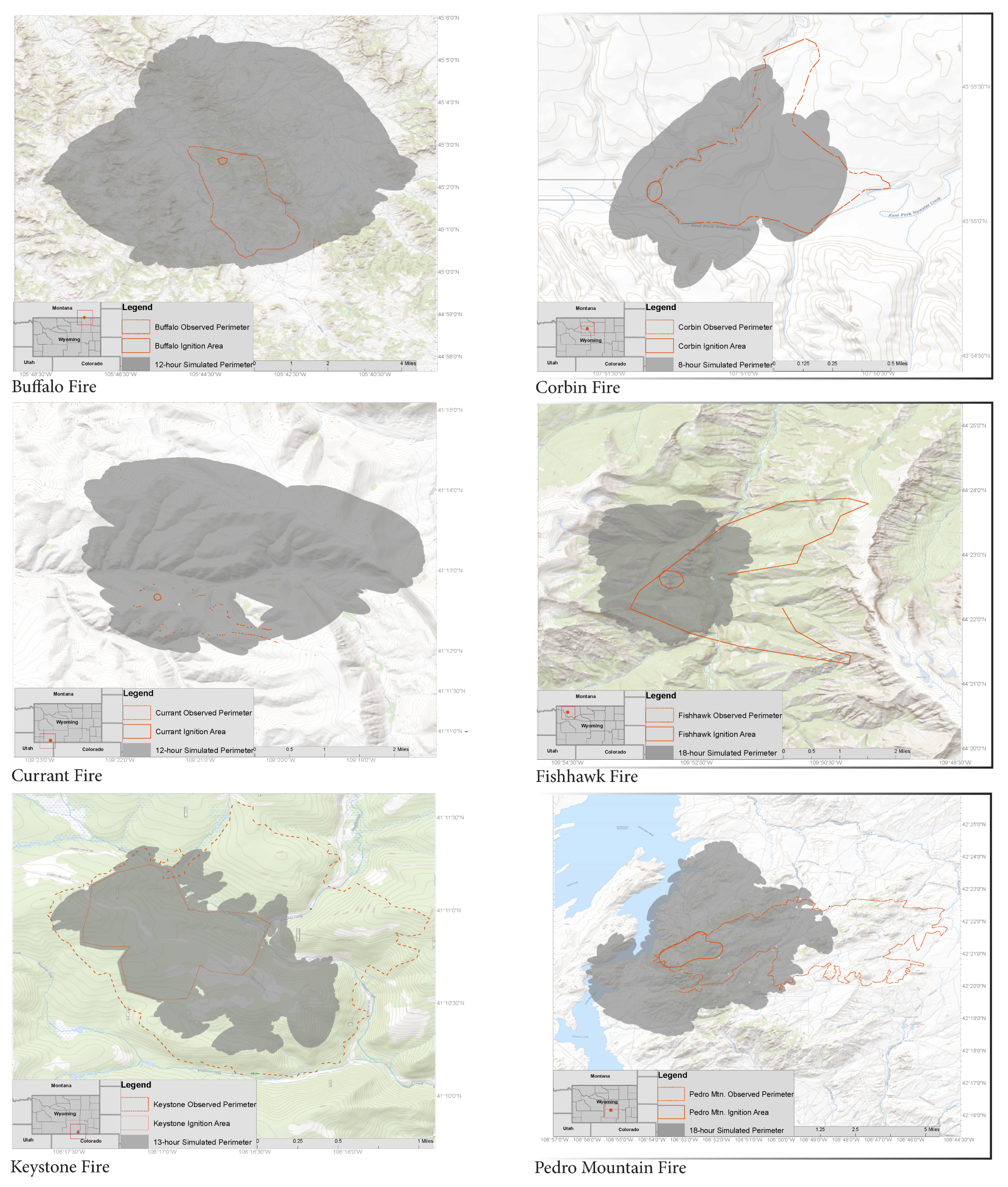
2.4. Wildfire Simulation

Two parameters are coded into the simulation configuration module that can be manually adjusted by individuals operating the model: (1) centroid distances (CD) of generated ellipses surrounding ignition points along the propagative front and (2) time step values in minutes for each iteration completed within a given Monte Carlo run. CD can be defined as the radius of each elliptical polygon generated from individual ignition points established along the flaming front. All simulations were configured to sixty-minute time steps, which is equal to one iteration of one Monte Carlo simulation. For this study, active wildfire perimeters were simulated from fire origination to ~eighteen hours due to availability constraints of the HRRR datasets and availability of their observed perimeter data (Table 2).
An idealized analysis was conducted to train the model and identify which CD value yielded the best performance results across all simulation environments [15]. A direct relationship between CD, dominant fuel loading model, and predictive accuracy was observed throughout this study. As CD increases, a subsequent decrease in predictive accuracy will occur in simulations of wildfires burning in higher fuel loads dominated by canopy fuels. In contrast, predictive accuracy increased when the CD was decreased for simulations of wildfires occurring within those higher canopy fuel loads. Through an iterative analysis, a mean CD of 5 m was identified as optimal across all fires and was used to achieve reported results for the rest of this study.
Simulations were run in Coordinated Universal Time (UTC) to align with the HRRR data format. For terminology purposes, one simulation predicts fire spread for the next x-number of hours. Intermediate or iterative predictions are generated on an hourly basis. Therefore, within a single simulation, there are x-number of iterations. One simulation consists of a simultaneous run of y-number of sample model configurations. Each model execution composed of a unique sample configuration is the equivalent to one Monte Carlo run. Simulated perimeters were evaluated against concurrent observed perimeters to assess variation in model performance for each target fire event. Performance of the WyoFire model was tested across a range of existing vegetation types, terrain complexity values, and fuel loading models in order to identify variables within each burnable environment that induce the greatest variance in the predictive performance of the model.

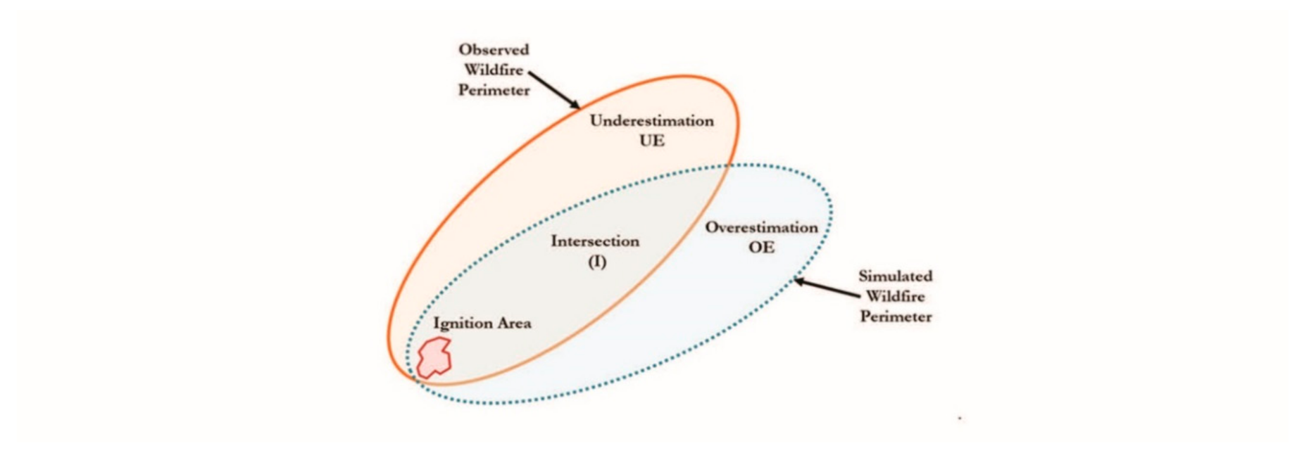
2.5. Assessing Model Performance

Simulation code was run across the High Performance Computing cluster (Teton), managed by the University of Wyoming’s Advanced Research Computing Center. Teton allowed multiple independent simulations to be run concurrently, distributed across multiple nodes, as well as scaling up the number of individual Monte Carlo simulations that could be run in parallel on individual nodes. Where a standard desktop could run 10 simulation queued sequentially, utilizing 4 or 8 cores at one time, the cluster enabled 10 (or more) simulations to be run concurrently, with up to 32 cores (i.e., 32 Monte Carlo simulations) running simultaneously on each node. Utilization of the cluster enabled both vertical (time to run a simulation) and horizontal (number of concurrent simulations) scaling, reducing the computational time from days down to hours. We used simultaneous batch processing of numerous wildfire simulations. Following the conclusion of all wildfire simulation jobs, logged results were transferred from the Linux system to a single-node workstation. Statistical and spatial analysis scripts were written in R-Studio. All data were graphed using R-Studio factoextra and ggplot2 packages. Simulated perimeter data were then analyzed to assess predictive performance by employing a series of spatial and statistical analyses using the aforementioned scripts. In order to calculate performance indices, a spatial intersection was conducted first to identify the critical areas of model Overestimation, Underestimation, and Intersection (Figure 2). The final burned area prediction was calculated using spatial overlay of all predicted wildfire perimeters obtained from each individual Monte Carlo simulation. The multipart polygons and individual polygons that were less than 1sq. meters were removed to generate the final predicted wildfire perimeter. The areas that were predicted to be burned only once were not included in the final perimeter. The results for each simulation were not compared amongst each other in this study due to the inherent randomness of the input weather and fuel conditions generated by the simulation. The resulting area of each predictive zone from the spatial intersection can then be integrated into a series of algebraic formulas to calculate performance indices that are indicative of overall model performance, e.g., Area Difference Index (ADI), Precision, Recall, and F1 Score.
ADI uses an index of incorrect estimation as a ratio of the correctly predicted area of intersection between the simulated and observed wildfire perimeters [6,8,16,17]. All performance indices calculations were conducted in R-Studio. ADI is calculated as:
A D I   t   =   O E   t   +   U E   t / I   t
ADI can also be decomposed into partial metrics which attempt to explain whether the source of the modelling error is a result of net Overestimation or Underestimation being the ADI of Overestimation (ADIoe) and the ADI of Underestimation (ADIue) [6,16]. The partial indices of ADIoe and ADIue are calculated as:
A D I u e   =   U E t / I t
A D I o e   =   O E t / I t
Precision and Recall are also considered in this study as partial metrics that combine to compose the F1 Score statistic [6,16]. Precision is functionally a measure of over-prediction, and Recall is functionally a measure of under-prediction [6,16]. Precision and Recall are calculated as:
P r e c i s i o n   =   I t / I t   +   O E t
R e c a l l   =   I t / I t   +   U E t
F1 Score is a measure of the overall state of agreement between the over- and underestimation of each simulated perimeter and is functionally equivalent to Sorensen’s Familiarity Index, which has been applied in pattern research but not in the discipline of fire science [6,8,16]. F1 Score functions as an evaluative index that essentially combines Precision and Recall values to assess the overall level of predictive agreement between simulated and observed perimeters [6,8,16]. F1 Score is calculated as:
F 1   =   2     I   t / I t   +   U E t   +   I t   +   O E t
Applying an appropriate combination of evaluative indices to assess the predictive performance of the model provides a foundation of computational results to conduct further analyses. Adhikari et al. [8] evaluated three 2017 wildfire events: (1) Keystone, (2) Pole Creek, and (3) Buffalo fires. Here, we apply a paralleled evaluation approach to an additional seven wildfires to increase the sample size and range in diversity of burnable environments tested. Computational results were analyzed in congruence with empirically derived modelling results, e.g., the morphology of predicted perimeters within a GIS platform to determine whether the accuracy of the fire spread model is sufficient for the application of wildfire education. Single-value performance metrics are useful when conducting rapid assessments of model performance for a particular simulation event, but they do not provide a sufficient level of detail regarding the sources of error within each simulation [6,18].

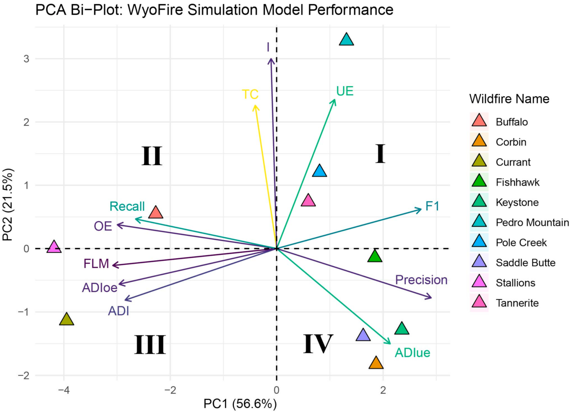
2.6. Principle Components Analysis

A Principal Components Analysis (PCA) was conducted on the simulation results to identify and understand the particular variables that might have induced the most variance on model performance and to identify emergent environmental properties of modeled fire events. Bi-plot visualizations were rendered using the factoextra package within R-Studio.

3. Results

3.1. Statistical Performance

We implemented a series of single-value performance metrics to evaluate how well WyoFire simulations performed across a range of landscapes (Figure 3). Each metric is a unitless index that represent specific facets of simulative model performance and can be formulated to determine rates of Overestimation, Underestimation, and Intersection for each series of the wildfire simulations. Mean performance indices for all simulations are found in Table 3. Performance outcomes for all simulations varied considerably between the 10 wildfire events. The Area Difference Index was designed as a simple metric to describe wildfire model performance, while the closer a value is to being equal to one suggests a less predictive error in simulation results in contrast to values much greater than one, which suggests more significant amounts of predictive modelling error [6,16]. Variables likely driving model over- or under-prediction in different environments are shown in Table 3.
Simulation of wildfire events occurring in environments with medium-to-high total fuel loadings dominated by shrubland and grassland vegetation types, such as the Currant, Stallions, and Buffalo fires, produced the highest rates of overestimation–underestimation (ADIoeADIue) (Table 3). In contrast, simulations of wildfire events occurring in environments with lower fuel loadings, dominated by mixed-forest, woodland, and shrub-steppe vegetation types, such as the Fishhawk, Saddle Butte, and Corbin fires, yielded the lowest rates of overestimation–underestimation. Wildfires that lie in mixed fuel types, Tannerite, Pole Creek, Pedro Mountain, and Keystone fires, displayed the most balanced performance in terms of overestimation and underestimation rates.

3.2. Principle Components Analysis

PCA was conducted on fuel characteristics and balance of predictive performance indices within each respective burnable environment. The first two principle components account for 78 percent of the total variance in model performance (Figure 4). The position of each fire relative to one another in the Bi-Plot (Figure 4) indicates the relative similarity of the models’ performance in predicting actual wildfire perimeters. Examining the burnable environment within each group also helps reveal what vegetation conditions yield over- and under-predictions by WyoFire. PCA yielded three distinct groups of wildfire events (Figure 4). Group 1 consists of the Corbin, Saddle Butte, Keystone, and Fishhawk fires, which can be observed in Quadrant IV of the Principle Components Analysis Bi-Plot. Group 2 is composed of the Currant, Stallions, and Buffalo fires, which can be seen in Quadrants II and III. Lastly, Group 3 consists of the Pole Creek, Tannerite, and Pedro Mountain fires, which can be found in Quadrant I.
The first Principal Component (PC-1) explains 56.6 percent of the variance in model performance across all simulations. Under-prediction indices were prominent along this axis, showing how the model performed within environments containing forested elements. Fuel loading became an emergent variable along this axis, while each group of individuals is ordered along the continuum by existing vegetation type and fuel-bed characteristics. The Fishhawk and Stallions fire simulations form the end members along the PC-1 axis. PC-1 appears to be primarily described by the existing vegetation type and dominant fuel loading models present within each respective burnable environment. WyoFire tended to under-predict in situations where the fuel load was low to medium with poor fuel-bed continuity. The Fishhawk Fire was characterized by low surface fuel loads but higher canopy fuel loads, as it occurred primarily in Rocky Mountain Subalpine Forest and Woodland vegetation types with a low total fuel loading. The Stallions Fire was primarily in North Western Great Plains Mixed Grass Prairie and Inter-Mountain Basin Big Sage Brush Steppe communities, possessing a low total fuel load and poor fuel-bed continuity.
Performance results for Fishhawk fire simulations displayed a much higher rate of underestimation than overestimation, while results for Stallions simulations show a relatively higher rate of overestimation than underestimation. The Fishhawk fire simulations had a greater rate of under-prediction in congruence with its high ratio of the canopy to surface fuels, further suggesting that this model may struggle to accurately model transitions of a flaming front propagating from the surface to canopy fuel types. Both wildfires burned across landscapes with average terrain complexity, as this variable did not prove to have a significant effect on the outcomes for these fire simulations.
The second Principle Component (PC-2) explains 21.5 percent of the variance in the predictive performance of the wildfire simulations. Certain burnable environments for wildfire simulations that possessed greater terrain complexity, meaning that the landscape has a greater degree of localized elevational variance, displayed overestimation rates similar to those with relatively low levels of terrain complexity, such as Pedro Mountain (6) and Corbin (2) fire simulations. Overestimation indices are pointed toward the Stallions, Currant, and Buffalo fire simulations as a result of simulating wildfire in higher fuel load with increased continuity. The Pedro Mountain and Corbin fires burned through similar environments dominated by Inter Mountain Basin Big Sage Brush Steppes and Artemisia tridentata ssp. vaseyana Shrubland Alliances, yet these two fires appear as opposing end members along the PC-2 axis. The significant difference between these two burnable environments is the influence of grassland vegetation present throughout the Corbin Fire but not the Pedro Mountain Fire.
The Pedro Mountain Fire had a strong influence of limber pine and juniper woodland vegetation types interwoven on the burnable landscape. This disparity may reflect that overall predictive performance results can be a product of the general fuel load and the specific fuel type present within the burnable environment. In this case, the presence-or-absence of canopy fuels may have been a driving factor of model error for these two wildfires. Heterogeneity of fuel loading models and the configuration of existing vegetation types across the landscape were the variables that induced the most significant amount of variance on performance results for each series of wildfire simulations.
Fires in Group 1 are characterized by low total fuel load and low degree of fuel-bed continuity, which resulted in higher rates of under-prediction. Simulation results for these four fires displayed the highest rates of under-prediction out of all model runs. The Corbin and Saddle Butte fires burned through sagebrush steppe and semi-arid shrubland vegetation types, while the Keystone and Fishhawk fires burned predominantly through Subalpine forest and woodland vegetation types such as spruce-fir, lodgepole pine, Douglas-fir, aspen, and other mixed conifers. Existing vegetation type(s) is the only significant difference amongst this grouping of individual wildfire environments, as variations in surface fuel loading appear to be the primary driver of model performance. It can be inferred that the most significant rates of under-prediction are yielded when simulating wildfire events in environments with high ratios of canopy-to-surface fuels. Given the discontinuous nature of sagebrush and semi-arid shrubland vegetation communities across the landscape, the interstitial spacing between clusters of burnable vegetation may result in simulations to under-predicting wildfire activity.
Group 2 is characterized by medium-to-high total fuel loadings and a high level of fuel-bed continuity, which resulted in higher rates of over-prediction. In contrast to Group 1, results for the simulations within Group 2 displayed the highest rates of over-prediction across all model simulations. The Buffalo, Currant, and Stallions fires burned in predominantly of Northwestern Great Plains mixed grassland and sagebrush steppe vegetation types. These landscapes are more homogeneous than landscapes present in Groups 1 and 3. Higher rates of overestimation are achieved when modelling wildfire propagation in herb- and grassland-dominated environments. The Currant and Stallions fire simulations yielded substantially higher rates of overestimation than did model runs for Buffalo Fire, which is likely attributable to the relatively lower level of surface fuel loading within the Buffalo Fire. We infer that higher rates of over-prediction are associated with simulative environments dominated by herb and grassland vegetation types with medium-to-high surface fuel loads. Simulations for wildfires that have burned on landscapes dominated by herb and grassland vegetation types possess a more continuous fuel bed, which results in a more uniform propagation pattern. The grassland vegetation types inherent to these simulation environments create a more continuous fuel bed than shrubland, forest, and woodland vegetation types do.
Group 3 is associated with low-to-medium fuel loads with varying levels of fuel-bed continuity, which resulted in a more accurate prediction with minimal over- or under-prediction. It can be inferred that these landscapes possessed a relatively higher degree of heterogeneity among existing vegetation types and fuel loadings due to the diversification of surface and canopy fuel types within these environments. All fires in this group were burned environments consisting of an increased mixture of canopy and surface fuel types. Tannerite Fire simulations yielded a higher rate of over-prediction than simulations of the Pole Creek and Pedro Mountain fires, as this is likely attributable to the presence of Montane–Foothill–Valley Grassland vegetation types across the burnable landscape for the Tannerite Fire. An increased level of heterogeneity among fuel types in these environments allows the model to simulate more transitionary events of the flaming front propagating from surface to canopy. Simulative results for the Pole Creek and Pedro Mountain fires displayed slightly lower rates of overestimation than the simulations for the Tannerite Fire.

4. Discussion

As the scope of wildfire activity and severity continues to increase [1], it has become increasingly important to identify and employ accurate predictive wildfire models to ensure timely interventions and protect property, lives, and biodiversity. In the Central Rocky Mountain Region, forest and woodland areas are typically characterized by steep and highly variable terrain elevation, which poses a series of complex challenges for wildfire models to resolve while integrating datasets with limited spatial resolutions. Our research quantified and evaluated the predictive performance of WyoFire, a Monte Carlo-based wildfire simulation model using a set of evaluative indices and corresponding PCA results to assess how the model performs over a range of diverse landscapes.
The different environments of the 10 wildfire events had unique vegetation type assemblages which helped bring about statistically significant variations in model performance. The significant variations in model performance were supported by statistically testing the accuracy results by using the equation ADIoeADIue to determine ranges in over- and underestimation within particular fuel types and loadings. Fuel loading was found to induce the most variance in model performance of all variables present within the wildfire simulations, while terrain complexity appeared to be the second most import factor on performance.
Simulations of wildfires occurring in shrubland- and grassland-dominated environments displayed the tendency to over-predict, while fire simulations of forested and woodland dominated-environments displayed the tendency to under-predict. In part, these performance differences may reflect interactions of the models used for wildfire spread in WyoFire [7,8,13,14], particularly during fuel condition changes (grassland to forest) or actual historic wind speeds used in our simulations as compared to modelled wind speed restrictions based on the source model assumptions [18,19,20]. This information is pertinent to researchers examining the processes of wildfire propagation across heterogeneous landscapes, as assumptions can be made about expected model performance across heterogeneous environments, as is evident by WyoFires’ output.
The results of this study reveal that, relative to vegetation type and fuel loading, terrain complexity has a minimal effect on predictive modelling performance when employing a Monte Carlo simulation approach. Rates of model overestimation and underestimation can be primarily attributed to fuel loading models and vegetation types within burnable environments. WyoFire displayed its highest rates of underestimation when simulating fires in environments with low surficial fuel loads that also have a low degree of fuel-bed continuity. These results are reasonable as wildfires burning within environments possessing lower degrees of fuel-bed continuity will invoke higher rates of under-prediction due to interstitial spaces between burnable vegetation [21]. In contrast, the highest rates of overestimation occurred when simulating wildfires in environments with medium-to-high total fuel loads that have a higher degree of fuel-bed continuity. This increased rate of overestimation likely occurred due to the increased connectivity of vegetation across the heterogeneous landscape [22]. These results will help us understand the environmental characteristics that lead to the tendencies for wildfire simulation models to over- or-under-predict wildfire behaviour. It should be noted that a range of centre distances should always be tested for each wildfire simulation environment in order to determine which value will yield the most accurate results. After analysing each of the ten fires within this study, we observed that parameterizing WyoFire with a higher CD yielded more favourable results in homogenous grasslands and shrubland landscapes. When parameterizing the model with a lower CD, we observed more favourable prediction results in forested and transitionary fuel types.
In its current state, WyoFire performs exceptionally well across a range of burnable environments as defined by fuel load, vegetation type and terrain complexity characteristics. The most adverse challenge faced in wildfire modelling is accounting for the stochastic nature of natural wildfire caused by internal dynamics, the ability to locally modify winds and fuels, coupled with mesoscale weather conditions that can shift rapidly. By employing a probabilistic approach that uses local historic variability to model wildfire propagation across heterogeneous landscapes, WyoFire incorporates natural stochasticity within each burnable environment. This approach begins to deal with the problem of wildfire simulation models coupled with meteorological forecast datasets maintaining accuracy due to the growth in error with each hour of prediction [23]. Monte Carlo simulation models that account for physical stochasticity within the natural environment are invaluable tools for a better understanding of how wildfires propagate across heterogeneous landscapes. Researchers leveraging deterministic wildfire prediction models for training purposes would benefit from implementing probabilistic Monte Carlo simulation models such as WyoFire.
WyoFire allows the user to parameterize specific model inputs to optimize the quality of predictive performance results regarding characteristics present within the desired burnable environment. If the characteristics associated with the burnable environment are known at the time of simulation, then a general hypothesis can be developed to address whether the simulation will result in over- or under-prediction. This model serves as a practical educational tool that can improve our understanding of wildfire behaviour in the lab and in the classroom. Future improvements to WyoFire largely hinge upon interpretations made from the results of this study, as conducting a comprehensive performance evaluation of model simulation results is pertinent for understanding its strengths and limitations [6,24].

5. Conclusions

In this study, we assessed the predictive performance of a Monte Carlo-driven wildfire simulation model, WyoFire, employing a set of single-value performance metrics and results from a Principal Components Analysis. Ten wildfire events in and around the state of Wyoming were simulated to assess the causes of variance in model performance which were mainly explained by existing vegetation types, fuel loadings, and degrees of terrain complexity variables. The PCA yielded three apparent groups of individual wildfire events based upon a measure of similarity between their resulting performance metric values and the physical characteristics that comprise each burnable environment. The fuel loading model emerged as the variable that induces the most substantial amount of variance on model performance when simulating wildfire events on a particular landscape, while terrain complexity was found to be relatively less significant in altering model performance.
Results from this research further confirm Adhikari et al.’s [8] finding that WyoFire is reliably effective and efficient across various heterogeneous landscapes. The model tends to over-predict fire spread in environments with a higher total fuel load in contrast to under-predicting wildfire activity in environments possessing lower total fuel loads. Results from all optimized simulations suggest that WyoFire performs exceptionally well, as accentuated rates of over- and under-prediction align with the fuel loading model and fuel-bed continuity present within the burnable environment. This model also displays the tendency to over-predict at higher rates when simulating wildfire events occurring on relatively smoother landscapes dominated by grassland vegetation types, in contrast to yielding substantially higher rates of under-prediction in environments dominated by shrubland and woodland vegetation types with a higher level of terrain complexity. WyoFires’ predictive ability across various fuel loading models and vegetation types may prove to be an effective tool to understand potential fire risk and potential processes that affect wildfire behaviour.

Author Contributions

Conceptualization, T.A.M., P.H., C.X.; methodology, B.A., C.W.O., T.A.M., P.H., C.X.; software, C.X., B.A., C.W.O., S.P.A.; formal analysis, C.W.O., S.P.A.; writing—original draft preparation, C.W.O., T.A.M., C.X., P.H., B.A., S.P.A. All authors have read and agreed to the published version of the manuscript.

Funding

This research received no external funding.

Conflicts of Interest

Authors declare no conflict of interest.

References

  1. Garfin, G.; Gonzalez, P.; Breshears, D.; Brooks, K.; Brown, H.; Elias, E.; Gunasekara, A.; Huntly, N.; Maldonado, J.; Mantua, N. Southwest. In Impacts, Risks, and Adaptation in the United States: Fourth National Climate Assessment; Reidmiller, D.R., Avery, C.W., Easterling, D.R., Kunkel, K.E., Lewis, K.L.M., Maycock, T.K., Stewart, B.C., Eds.; U.S. Global Change Research Program: Washington, DC, USA, 2018; Volume II, pp. 1101–1184. [Google Scholar]
  2. Westerling, A.L. Increasing western US forest wildfire activity: Sensitivity to changes in the timing of spring. Philos. Trans. R. Soc. B Biol. Sci. 2016, 371, 20150178. [Google Scholar] [CrossRef] [PubMed]
  3. Stavros, E.N.; Abatzoglou, J.T.; McKenzie, D.; Larkin, N.K. Regional projections of the likelihood of very large wildland fires under a changing climate in the contiguous Western United States. Clim. Chang. 2014, 126, 455–468. [Google Scholar] [CrossRef]
  4. Higuera, P.E.; Abatzoglou, J.T. Record-setting climate enabled the extraordinary 2020 fire season in the western United States. Glob. Chang. Biol. 2020. [Google Scholar] [CrossRef] [PubMed]
  5. McWethy, D.B.; Schoennagel, T.; Higuera, P.E.; Krawchuk, M.; Harvey, B.J.; Metcalf, E.C.; Schultz, C.; Miller, C.; Metcalf, A.L.; Buma, B. Rethinking resilience to wildfire. Nat. Sustain. 2019, 2, 797–804. [Google Scholar] [CrossRef]
  6. Duff, T.J.; Chong, D.M.; Tolhurst, K.G. Indices for the evaluation of wildfire spread simulations using contemporaneous predictions and observations of burnt area. Environ. Model. Softw. 2016, 83, 276–285. [Google Scholar] [CrossRef]
  7. Rothermal, R. A Mathematical Model for Predicting Fire Spread in Wildland Fuels; Intermountain Forest & Range Experiment Station, Forest Service, US Department of Agriculture: Ogden, UT, USA, 1972; 40p. [Google Scholar]
  8. Adhikari, B.; Xu, C.; Hodza, P.; Minckley, T.A. Developing a geospatial data-driven solution for rapid natural wildfire risk assessment. J. Appl. Geogr. In Revision.
  9. Bennett, N.D.; Croke, B.F.; Guariso, G.; Guillaume, J.H.; Hamilton, S.H.; Jakeman, A.J.; Marsili-Libelli, S.; Newham, L.T.; Norton, J.P.; Perrin, C. Characterising performance of environmental models. Environ. Model. Softw. 2013, 40, 1–20. [Google Scholar] [CrossRef]
  10. Kelso, J.K.; Mellor, D.; Murphy, M.E.; Milne, G.J. Techniques for evaluating wildfire simulators via the simulation of historical fires using the Australis simulator. Int. J. Wildland Fire 2015, 24, 784–797. [Google Scholar] [CrossRef] [Green Version]
  11. Adhikari, B. A Web GIS Portal for Modeling Wildfire Spread in Near Realtime and Assessing Associated Risk; University of Wyoming: Laramie, WY, USA, 2018. [Google Scholar]
  12. Filippi, J.B.; Mallet, V.; Nader, B. Representation and evaluation of wildfire propagation simulations. Int. J. Wildland Fire 2014, 23, 46–57. [Google Scholar] [CrossRef]
  13. Wagner, C.V. Conditions for the start and spread of crown fire. Can. J. For. Res. 1977, 7, 23–34. [Google Scholar] [CrossRef]
  14. Finney, M.A. FARSITE: Fire Area Simulator—Model Development and Evaluation; Research Paper RMRS-RP-4 Revised; USDA Forest Service, Rocky Mountain Research Station: Ogden, UT, USA, 2004; 47p. [Google Scholar]
  15. Ott, C.W. Performance Evaluation of a Monte Carlo Driven Wildfire Simulation Model: Assessing Model Performance to Advance Education and Improve Human Safety; University of Wyoming: Laramie, WY, USA, 2020. [Google Scholar]
  16. Fawcett, T. An introduction to ROC analysis. Pattern Recognit. Lett. 2006, 27, 861–874. [Google Scholar] [CrossRef]
  17. Pugnet, L.; Chong, D.; Duff, T.; Tolhurst, K. Wildland–urban interface (WUI) fire modelling using PHOENIX Rapidfire: A case study in Cavaillon, France. In Proceedings of the 20th International Congress on Modelling and Simulation, Adelaide, Australia, 1–6 December 2013; pp. 1–6. [Google Scholar]
  18. Duff, T.J.; Cawson, J.G.; Cirulis, B.; Nyman, P.; Sheridan, G.J.; Tolhurst, K.G. Conditional performance evaluation: Using wildfire observations for systematic fire simulator development. Forests 2018, 9, 189. [Google Scholar] [CrossRef] [Green Version]
  19. Moon, K.; Duff, T.; Tolhurst, K. Sub-canopy forest winds: Understanding wind profiles for fire behaviour simulation. Fire Saf. J. 2019, 105, 320–329. [Google Scholar] [CrossRef]
  20. Andrews, P.L.; Cruz, M.G.; Rothermel, R.C. Examination of the wind speed limit function in the Rothermel surface fire spread model. Int. J. Wildland Fire 2013, 22, 959–969. [Google Scholar] [CrossRef]
  21. Loehle, C. Applying landscape principles to fire hazard reduction. Forest Ecol. Manag. 2004, 198, 261–267. [Google Scholar] [CrossRef] [Green Version]
  22. Kerby, J.D.; Fuhlendorf, S.D.; Engle, D.M. Landscape heterogeneity and fire behavior: Scale-dependent feedback between fire and grazing processes. Landsc. Ecol. 2007, 22, 507–516. [Google Scholar] [CrossRef]
  23. Coen, J.L.; Schroeder, W. Use of spatially refined satellite remote sensing fire detection data to initialize and evaluate coupled weather-wildfire growth model simulations. Geophys. Res. Lett. 2013, 40, 5536–5541. [Google Scholar] [CrossRef]
  24. Salis, M.; Arca, B.; Alcasena, F.; Arianoutsou, M.; Bacciu, V.; Duce, P.; Duguy, B.; Koutsias, N.; Mallinis, G.; Mitsopoulos, I. Predicting wildfire spread and behaviour in Mediterranean landscapes. Int. J. Wildland Fire 2016, 25, 1015–1032. [Google Scholar] [CrossRef]
Figure 1. Distribution of 2017 and 2019 Wyoming and Montana fire events used in this study.
Fire 03 00071 g001
Figure 2. Graphical representation of the observed and simulated wildfire perimeters, as well as the three predictive areas, underprediction, intersection and overprediction, that are a product of each simulation, adapted from Duff, Chong, and Tolhurst [6].
Fire 03 00071 g002
Figure 3. Maps of showing ignition polygon, fire perimeter (actual) and 18-h simulated fire perimeter for each of 10 fires modelled in this study.
Fire 03 00071 g003aFire 03 00071 g003b
Figure 4. Principal Components Analysis (PCA) Bi-Plot of variable weightings and coordinate locations of individual wildfire events. The events are color-coded and symbolized by triangles within the Bi-Plot. FLM = Fuel Loading Model, TC = Terrain Complexity, ADI = Area Difference Index, OE = Overestimation, UE = Underestimation, ADIoe = ADI of Overestimation, ADIue = ADI of Underestimation. These variables are represented by individual arrow vectors of varying lengths and colors, in which a lengthier vector signifies that the variable is better represented within the analysis and a darker color fill indicates a better Quality of Representation (cos2).
Fire 03 00071 g004
Table 1. Metadata of datasets used to simulate wildfire events, adapted from Adhikari et al. [8].
Resolution
DatasetSourceData Volume (Gigabyte/Iteration)Spatial
(m)
Temporal (h)
High-Resolution Rapid Refresh (HRRR) NOAA11.530001
VIIIRS Active Fire Hotspot NASA0.0237512
Dead Fuel MoistureWSFD/USFS1250024
Digital Elevation ModelUSGS2610Updated: January 2017
Vegetation and Fuels LANDFIRE3.530Updated: January 2014
Historical Wildfire Perimeter (Observed)USGS GeoMAC0.1N/A24
Historical HRRR DataUni. Of Utah9300024
Table 2. Simulation parameters for the ten wildfires analyzed within this study.
WildfireTotal Size (Acres)Simulation Duration (h)Observed Perimeter SourceTotal Simulations (n)
Keystone, 2017110213VIIRS600
Pole Creek, 2017213912GeoMAC and VIIRS600
Buffalo, 2017351512GeoMAC and VIIRS600
Stallions, 2017111112VIIRS600
Tannerite, 2019134918GeoMAC600
Pedro Mountain, 2019938818GeoMAC and VIIRS600
Currant, 201938112GeoMAC600
Corbin, 20191648GeoMAC600
Fishhawk, 2019235918GeoMAC and VIIRS600
Saddle Butte, 201925212GeoMAC600
Total Simulations6000
Table 3. Mean performance index values derived from all wildfire simulations based on the optimal Centroid Distance of five meters.
WildfireExisting Vegetation Type(s)Terrain RoughnessADIoeADIueFuel Loading
CurrantGrassland, Shrubland337.940Med—High
StallionsNorthwestern Great Plains Grassland, Ponderosa-Pine Forest632.430Med–High
BuffaloNorthwestern Great Plains Grassland, Sage Brush Steppe38.479Low–Med
TanneriteSage Brush Steppe, Montane–Foothill–Valley Grassland51.481Low–High
Pole CreekSpruce-Fir Woodland, Aspen and Mixed-Conifers71.031Low–Med
Pedro MountainSage Brush Shrubland, Limber Pine-Juniper Forest6−0.093Low–Med
KeystoneLodgepole Forest, Spruce-Fire Woodland, Aspen and Mixed Conifers1−1.733Low–Med
FishhawkSubalpine Woodland, Spruce-Fir Woodland, Douglas-Fir Forest5−2.450Low
Saddle ButteSage Brush Shrubland, Sage Brush Steppe, Montane Meadow4−2.789Low
CorbinSage Brush Steppe, Sage Brush Shrubland, Semi-Desert Shrub Steppe2−4.248Low
Publisher’s Note: MDPI stays neutral with regard to jurisdictional claims in published maps and institutional affiliations.

