Generation and Mapping of Fuel Types for Fire Risk Assessment

Abstract

Fuel mapping is key to fire propagation risk assessment and regeneration potential. Previous studies have mapped fuel types using remote sensing data, mainly at local-regional scales, while at smaller scales fuel mapping has been based on general-purpose global databases. This work aims to develop a methodology for producing fuel maps across European regions to improve wildland fire risk assessment. A methodology to map fuel types on a regional-continental scale is proposed, based on Sentinel-3 images, horizontal vegetation continuity, biogeographic regions, and biomass data. A vegetation map for the Iberian Peninsula and the Balearic Islands was generated with 85% overall accuracy (category errors between 3% and 28%). Two fuel maps were generated: (1) with 45 customized fuel types, and (2) with 19 fuel types adapted to the Fire Behaviour Fuel Types (FBFT) system. The mean biomass values of the final parameterized fuels show similarities with other fuel products, but the biomass values do not present a strong correlation with them (maximum Spearman’s rank correlation: 0.45) because of the divergences in the existing products in terms of considering the forest overstory biomass or not.

1. Introduction

Wildland fires play an important role in the dynamics of terrestrial ecosystems. Although they have positive effects on biodiversity and plant succession [1], wildland fires are also a critical disturbance factor in forests, affecting the structure, function [2], adaptation, and distribution [3] of ecosystems, as well as degradation of water quality, erosion, and land cover change [4,5]. In addition, wildland fires constitute a serious threat to the environment and society when they are not well managed [6,7,8]. It is estimated that 4–4.5 million km² is burnt annually in the world [9,10], but this estimation is most likely conservative. These areas include agricultural and pasture burns, and wildland fires, which have a strong impact on societal and economic value. This is particularly clear in Southern Europe (Spain, Portugal, Greece, Southern France), where most European fires occur, but these patterns may be extended to Northern Europe as a result of global warming [11,12]. In fact, Europe’s wildland fire vulnerability has recently increased due to the effects of climate change [13,14,15].

The origin of wildland fires can be natural (mainly lightning) or human. For fires to spread, continuity of living or dead vegetation is required to maintain the fire, as well as oxygen and heat transfer for ignition. Moreover, suitable environmental, meteorological, and topographic conditions must be met [16]. Fuel types, which refer to vegetation categories with similar behaviour in fire propagation [17], are a primary factor in the behaviour of wildland fires and their prevention [18,19]. Consequently, mapping fuel types is critical to characterize risk conditions and plays an important role in wildland fire risk prevention, where it is essential to have quality maps that are easily and regularly updated. Fuel parameterization is performed throughout fuel models, which are numerical descriptions of the physical parameters of each fuel type. Fuel models involve parameterizing fuel types to estimate their fire behaviour. They are widely used in fire risk assessment and behaviour programmes [20,21]. Many efforts have been made to develop methodologies to generate and map fuel types. The methods used to obtain fuel types and their parameters strongly depend on their input data, final use, and the detail of the work scale [16,20].

Mapping the updated distribution of fuels and describing their properties improves decision-making, evaluation, and risk management of wildland fires because it considers vegetation changes due to previous fires and the dynamic nature of forest fuels [16,22,23]. Currently, the problem is the development of cost-efficient methods for updating fuel maps and their parameters, which will be used in fire behaviour modelling [16,24]. Therefore, it is essential to improve the current fuel mapping methodologies to amend wildland fire assessment, by providing an optimal allocation of resources [25,26,27,28] to mitigate the adverse effects of wildland fires through early response and strategic planning [16].

The vegetation characteristics that are usually considered when describing fuel types are crown height, crown base height, percentage of vegetation covered area, forest canopy density (proportion of the ground covered by the projection of the crown of the trees to the ground), apparent crown density, canopy bulk density (mass of available canopy fuel per canopy volume unit), number of trees by area, vertical and horizontal continuity, moisture content, live and dead fuel load, and biomass [16,20]. Standardized fuel classification systems based on vegetation characteristics have been proposed in recent decades for several world regions: Southeast Asia [26], United States [21,29], Canada [30], and the Mediterranean region [24,31]. One of the most used is the Fire Behaviour Fuel Types (FBFT) [21], prepared by the United States Forest Service Rocky Mountain Research Station for the United States. It uses field measures and photo series to describe 40 fuel types based on the 13 types of the Northern Forest Fire Laboratory (NFFL) system [29], widely used for fire propagation modelling [19,24]. FBFT [21] improves the accuracy of fire behaviour predictions for surface fires outside the fire season (June–October). It also considers the humidity of the climate in which the fuel is included. Some works have adapted the FBFT fuel types to European islands [32,33].

The original 40 FBFT fuel types are divided into seven large groups: grass (GR), grass-shrub (GS), shrub (SH), timber-understory (TU), timber-litter (TL), slash-blowdown (SB), and non-burnable (NB). For each fuel type, the parameters to be used in fuel and fire propagation models are defined, except for the NB category. For each fuel type, the system provides an estimation of the fuel load, fire spread rate, and flame length based on generic climatic conditions [21]. The fuel load refers to the amount of fuel potentially available for combustion [20]. The fire spread rate is the rate of the fire head advance [34]. The flame length is the distance between the midpoint of the flame depth at the base of the flame and the flame tip [35].

Traditionally, field samples, photointerpretation of aerial images, and remote sensing methods have been used to perform mapping of fuel types and their parameterization. Recent bibliographic reviews [36,37] show a growing utilization of remote sensing for fire risk assessment, using passive optical sensors, Radio Detection And Ranging (RADAR), and Laser Imaging Detection And Ranging (LiDAR) (including ground, airborne, and satellite systems [38]). Remote sensing presents the advantages of global systematic coverage (easily updateable) and information on non-visible regions of the spectrum [16,20]. Remote sensing has mainly contributed to characterizing the conditions of fuel types—moisture content, biomass, canopy coverage, and vertical and horizontal continuity—evidencing the considerable capabilities of this technique in evaluating the multiple variables involved in fire risk assessment. A common approach to fuel mapping using remote sensing is to firstly map the vegetation types and secondly generate the fuel types using auxiliary information to refine the vegetation types [36]. Second-order variables, such as fire spread rate and flame length, have also been mapped [39].

At the local-regional scale, the input data to classify fuel types have usually been generated using optical remote sensing images. Their high temporal resolution facilitates the updating of the derived cartography, although they require calibration and validation efforts. The most used sensors have been Landsat Thematic Mapper (TM) [31,40,41] and Sentinel-2 MultiSpectral Instrument (MSI) [42,43,44]. High spatial resolution sensors, such as those onboard the QuickBird [39,45,46] and WorldView-2 [47,48] satellites, have also been used. Visible, NIR, and SWIR bands, spectral indexes [32,39,41,42,45,49,50], and multi-temporal analysis [31,43] have also been used, which have provided classification improvements [51]. Different classification algorithms have been used: maximum likelihood [31,46], decision trees [39], random forest [42], Support Vector Machine (SVM) [42], and Object Based Image Analysis (OBIA) [43,44,45].

At the continental-global scale, cartography of fuel types has usually been generated from the integration of land use databases and pre-existing maps as input data. However, using databases does not consider phenological changes. There are examples of continental-scale works (South America [52] and Africa [53]) that generate fuel maps from the integration of databases and pre-existing products. With a similar approach, a global fuel type map was recently proposed [54] by combining land cover and biogeographic region databases with optical remote sensing-derived products for tree vegetation, such as vegetation continuous field collection 5 from Terra MODIS (Moderate Resolution Imaging Spectroradiometer).

The main objective of this work is to develop a methodology to map fuel types at a regional scale for modelling fire propagation behaviour. We selected the FBFT system [21] because it provides a standard set of parameters for fire behaviour estimation. This work is focused on the Iberian Peninsula and the Balearic Islands but aims to extend similar methods to other European regions. We first describe the methods used to generate the vegetation map. Then, we describe the methods used to generate the map of fuel types and the parameters for the different fuel types. Since validation of the fuel map was not feasible, we present a first assessment of the result by comparing the fuel parameters with those derived from a European fuel map produced under the European Forest Fire Information System (EFFIS) programme [55] and a global product derived from [54]. This work is part of the European project FirEUrisk, which aims to generate a European integrated strategy for fire risk assessment, reduction, and adaptation.

2. Materials and Methods

2.1. Study Case: Spatial Delimitation

The study area is the Iberian Peninsula and the Balearic Islands, with 587,198.93 km² (Figure 1). Other archipelagos belonging to Spain and Portugal were not considered to focus the work on the European Mediterranean region. Wildland fires in European Union countries for the 2000–2017 period have affected 480,000 ha/year, 34 people/year, and have implied costs of 3 billion euros/year [56]. The Mediterranean European countries are the most affected by wildland fires, with an annual average of about 45,000 wildland fires and 478,900 burnt hectares. Spain and Portugal have been for decades the two countries in Europe most affected by wildland fires, especially in the fire season (June–October). For 2009–2018, the average annual statistics were 12,182 fires and 99,083 burnt hectares for Spain, and 18,345 fires and 138,841 hectares for Portugal [15,57,58,59].

A relationship between fires in the Iberian Peninsula and its long-term climatic conditions has been observed [62]. The study area has three biogeographic regions, which are stable over time (Figure 1): (1) Alpine, with a high mountain climate, (2) Atlantic, with mild temperatures and humid summers, and (3) Mediterranean, characterized by hot and dry summers. Their different climatic conditions favour different degrees of vegetation development [63], and therefore different fuel types.

2.2. Materials, Data, and Analysis Techniques

The development of the cartography and characterization of fuel types was based on the integration of multi-seasonal images (spring, summer, autumn) of the Sentinel-3 Synergy product, MODIS vegetation continuous field collection 6 maps, a map of biogeographic regions, and a biomass map. Two main steps were followed: (1) the generation of the basic vegetation cartography, and (2) the generation of the cartography of fuel types (Figure 2).

2.2.1. Generation of the Basic Vegetation Cartography

To avoid relying on external land cover maps as in [52,53,54] and to base our approach on updated data, a vegetation map was generated from Sentinel-3 Synergy product images. Sentinel-3 is part of the European Space Agency’s (ESA) Copernicus programme [64] and was conceived for land monitoring and security applications, and climate change detection [65]. It is composed of a pair of optical satellites, Sentinel-3A and 3B, in orbit since 2016 and 2017, respectively. It includes two main instruments: OLCI (Ocean and Land Colour Instrument, 21 channels, 300 m spatial resolution) and SLSTR (Sea and Land Surface Temperature Radiometer, 9 channels, 500 m resolution). Sentinel-3 images have already been used for wildland fire detection and mapping. Works exist that analyse the capabilities of the Sentinel-3 SLSTR sensor for active fire detection [66,67,68,69], especially for forest biomass burning events [66].

In this, work, the Sentinel-3 Synergy product [65] was used, as it combines OLCI and SLSTR data. This product offers geometrically, atmospherically, and Top of Canopy (TOC) reflectivity corrected daily images at 300 m resolution for 26 spectral bands. The Sentinel-3 Synergy product has already been used, in combination with other Sentinel-3 products, for the generation of a moderate spatial resolution global burnt area product under the ESA’s Fire Climate Change Initiative (CCI) project [70]. However, the potential of this product to contribute to fuel modelling and mapping has not been exploited yet. In this work, we aim to use the relatively recent product of Sentinel-3 Synergy in the context of fuel modelling, especially for the generation of updated vegetation maps, which are expected to be useful for fuel mapping.

Sentinel-3 Synergy images were downloaded from the Copernicus Open Access Hub [71] for the study area: 20 images for summer 2020, 27 images for autumn 2020, and 20 images for spring 2021. For each season, cloud-free mosaics were performed at 300 m resolution in SNAP 7.0 (Sentinel Application Platform), which uses the nearest neighbour (Figure 3). The mosaics were projected from WGS84 Geographic latitude/longitude coordinates to ETRS89 Albers equal-area conic projection with central meridian in 3° W, which preserves the area measure, and is appropriate to represent the study area.

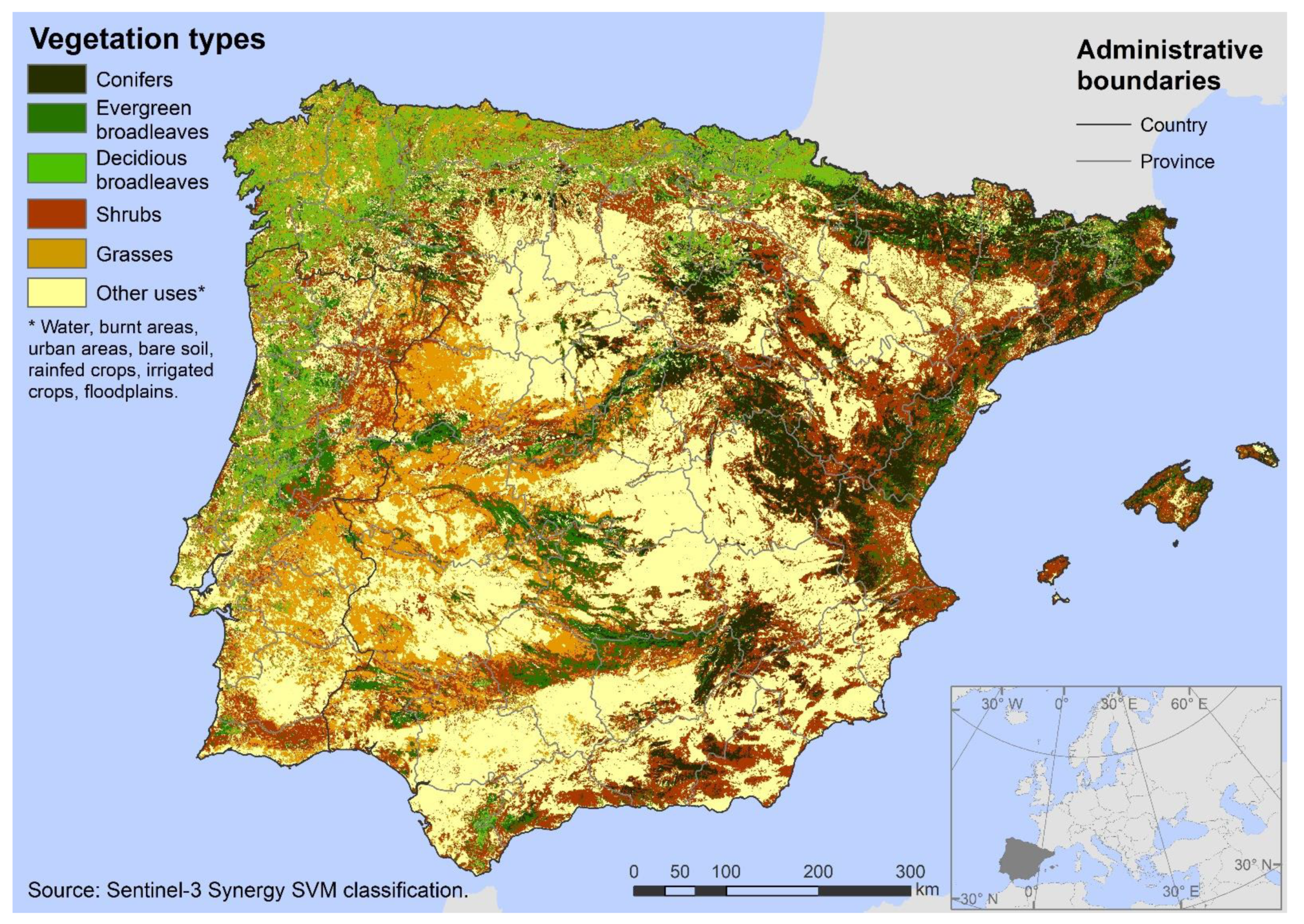
We selected the following categories to create the vegetation map: conifers, evergreen broadleaves, deciduous broadleaves, shrubs, grasses, and other uses. In the study area, the conifers only refer to evergreen conifers because deciduous conifers only grow in boreal climates. However, broadleaves can be evergreen or deciduous [63]. Conifers, evergreen broadleaves, and deciduous broadleaves have different moisture content and amount of leaves in summer and winter, and therefore different responses to fire [72]. The other uses category refers to non-natural vegetation surfaces, including crops. This classification was selected for an easy adaptation to the FBFT system [21].

(A)

Classification training sample

First, a total of 403 pure training pixels were visually selected with the help of Google Earth for 14 initial categories: conifers, evergreen broadleaves, Atlantic deciduous broadleaves, Mediterranean deciduous broadleaves, landa (Atlantic shrubs), thermophilic Mediterranean shrubs, grasses, water, burnt areas, urban areas, bare soil, rainfed crops, irrigated crops, and floodplains. These categories consider the variability of land use and vegetation due to the biogeographic regions of the study area.

(B)

Input bands

A total of 21 bands were used as classification input. For each season, 5 nadir observation bands (which minimize geometric distortions) were used: 555 nm (green), 659 nm (red), 865 nm (NIR), 1610 nm (SWIR 1), 2250 nm (SWIR 2). These spectral regions have been widely used in previous studies [32,41,42,49,50,51] as they have shown the potential to discriminate vegetation types. To improve the classification performance, the NDWI index ((NIR band − SWIR 2 band)/(NIR band + SWIR 2 band)) and the SAVI index (((NIR band − Red band)/(NIR band + Red band + L)) * (1 + L)) were also calculated for each season and used as input bands. We used the standard soil brightness correction parameter L = 0.5 [73,74,75].

(C)

Classification algorithm

The classification was performed using Support Vector Machine (SVM), a supervised non-parametric statistical machine learning algorithm, for the 403 pure training pixels and the 21 input bands. It finds the optimal hyperplane to separate the input dataset into the categories defined by the training sample [76]. The classification was performed in Orfeo ToolBox of QGIS 3.10 assigning the most similar category to each pixel. We used SVM kernel RBF (Radial Base Function), which offers optimal results for classifying vegetation with remote sensing [76], and cost parameter 100 [42]. The classification was also performed using random forest. As in [42], 100 trees and 3 as the minimum number of samples per node were used. Then, some classified categories were merged to fit the final target categories (

Table 1. Merger of categories.

Initial Training Categories	Final Target Categories
Conifers	Conifers
Evergreen broadleaves	Evergreen broadleaves
Atlantic deciduous broadleaves, Mediterranean deciduous broadleaves	Deciduous broadleaves
Landa, thermophilic Mediterranean shrubs	Shrubs
Grasses	Grasses
Water, burnt areas, urban areas, bare soil, rainfed crops, irrigated crops, floodplains	Other uses

).

(D)

Validation

The vegetation map was validated using as the reference a mosaic of TOC reflectivity images from the Sentinel-2 MSI sensor (resolution 20 m) for the same period as the Sentinel-3 images. A validation dataset was generated for 500 independent validation points, which were selected by stratified random sampling (this compensates for differences in surface area covered by each category). A vector net of the dimensions of the classified image (300 m × 300 m) was generated, and each point was visually assigned to the category with the largest extension of the Sentinel-2 reference mosaic in the square of the net in which it is included (Figure 4). Visual qualitative analysis was also performed, comparing with (1) the Sentinel-2 reference mosaic and (2) vegetation maps for the study area [63,77].

2.2.2. Generation of the Cartography of Fuel Types

To facilitate the integration of the raster vegetation map with the auxiliary maps, the vegetation map was vectorized to obtain vegetation polygons. Non-vegetation categories (other uses: water, burnt areas, urban areas, bare soil, rainfed crops, irrigated crops, and floodplains) were not considered. The vegetation map was integrated with data of vegetation horizontal continuity [78] and biogeographic regions [60]. The resulting fuel map was reclassified to obtain the target FBFT categories [21].

(A)

Horizontal fuel continuity

Horizontal fuel continuity is considered an important factor influencing fire behaviour [16] and therefore is commonly considered in the classifications of fuel types [54]. We used 2019 global MODIS vegetation continuous field collection 6 version 1 [78]. This dataset indicates the percentage of tree and non-tree vegetation cover (0–100%) at 250 m resolution with 7.87–9.40% mean absolute error [79]. A mosaic of the study area was performed and projected to ETRS89 Albers equal-area conic projection with central meridian in 3° W.

The 5 vegetation categories of the vegetation map were split into tree (conifers, evergreen broadleaves, deciduous broadleaves) and non-tree (shrubs, grasses) categories. For each vegetation polygon, zonal statistics (mean and standard deviation) were calculated for (1) the percentage of tree vegetation cover for the tree categories and (2) the percentage of non-tree vegetation cover for the non-tree categories. Afterwards, the horizontal continuity percentage was used to divide each vegetation type into categories according to their fire spread occurrence possibility: (1) 0–40%, (2) 40–70%, and (3) 70–100%. The 0–40% category refers to sparse vegetation cover density. The 40% threshold was assigned because it is the percentage used in the Fire Characteristic Classification System (FCCS) to decide if canopy fire spread can occur. To divide the rest of the cover percentage, the 70% threshold was assigned. The 40–70% category refers to dense cover density, while the 70–100% category refers to very dense cover density [43,54].

(B)

Biogeographic regions

Environmental and climatic conditions affect fire spread [16], as a relationship between fires in the study area and its long-term climatic conditions has been observed [62]. Moreover, differences in species richness [80,81], total fuel biomass [82,83,84,85], and fire behaviour [86,87] within biogeographic regions have also been shown. To account for the biomass variations of fuels in our study area, we used the 2016 dataset of Europe’s biogeographic regions generated by the European Environment Agency (EEA) [60]. The study area was divided into Alpine, Atlantic, and Mediterranean regions (Figure 1). Through overlapping, each polygon with a given vegetation type and horizontal continuity percentage was assigned the biogeographic region in which it was included. If a polygon belonged to more than one biogeographic region, it was split into as many polygons as biogeographic regions it belonged to.

(C)

Generation of the customized Iberian fuel types

Polygons with the same vegetation type, percentage of horizontal vegetation cover group, and biogeographic region were merged to generate the customized Iberian fuel types. Therefore, the description of each Iberian fuel type is based on its vegetation type, horizontal continuity percentage, and biogeographic region. The Iberian fuel types were mapped to create the Iberian fuel map. The fuel types’ area, and their horizontal continuity mean and standard deviation were calculated.

(D)

Adaptation of the Iberian fuel types to the FBFT system

The Iberian fuel types were adapted to the fuel categories of the FBFT system [21]. We based this translation on the different fuel types’ definitions, using the variables of vegetation type, climatic conditions, and horizontal fuel continuity. The vegetation type is both defined in the Iberian and standard FBFT fuel types. For the Iberian fuel types, we derived this information from the SVM classification of the Sentinel-3 Synergy mosaics, while for the FBFT system, this information is derived from field work and photo series. The climatic conditions are defined by the biogeographic regions for the Iberian fuel types (distinguishing 3 regions for the study area from [60]), while the FBFT system only distinguishes between fuel types from sub-humid/humid climates (adequate rainfall in all seasons) and arid/semi-arid climates (rainfall deficit in summer). Because the FBFT system only distinguishes between sub-humid/humid and arid/semi-arid climates, we assigned the study area’s Alpine and Atlantic fuels to the sub-humid/humid group and the Mediterranean to the arid/semi-arid group. The horizontal fuel continuity information is derived from the dataset of [78], and for the FBFT system, information on fuel density and load is based on field measures and photo series. We also visually analysed the United States FBFT map [88], extracting similar covers to those existing in the study area. The input data caused some Iberian fuel types to be assigned to various FBFT fuels. However, not all original FBFT fuels were found in the study area. The FBFT-adapted fuel mapping generated the FBFT fuel map. To improve this map’s readability, the non-burnable categories were not mapped (not considered fuel).

Then, the parameters from the original FBFT fuel types were translated to the FBFT-adapted fuel types for the study area. For each fuel type, mean biomass load, spread rate, and flame length values (

Table A1. Predictive fire behaviour intensity categories for surface fires. Adapted from [21].

Intensity Category	Rate of Spread (m/min)	Flame Length (m)
Very low	0–0.30	0–0.31
Low	0.30–0.75	0.31–1.22
Moderate	0.75–3.00	1.22–2.44
High	3.00–7.50	2.44–3.66
Very high	7.50–22.5	3.66–7.62
Extreme	>22.5	>7.62

in the Appendix A) were extracted from the original FBFT fuel descriptions. These values refer to the mean fuel conditions and serve to predict fire behaviour inside and outside the fire season (June–October). Local and short-term variations in fire risk caused by changes in the weather conditions and the amount of fuel moisture, among other variables, are expected to be considered in posterior analysis for fire behaviour modelling. FBFT describes the total surface biomass for non-tree fuels and only timber litter and understory biomass for tree fuels [21]. Fire potential spread rate and flame length were mapped. The FBFT fuel types were characterized by their FBFT category, area, biomass, potential spread ratio, and potential flame length.

2.2.3. Fuel Parameters: Biomass

For tree-vegetation fuels, original FBFT biomass load descriptions only refer to timber litter and understory [21], which affect surface fires. Thus, further analysis was performed to obtain the biomass load that would affect crown fires. We completed biomass load values from the original FBFT descriptions with the 2018 global CCI (Climate Change Initiative) Biomass dataset [89], recently made available. This product was derived from observations from the Copernicus Sentinel-1, Envisat’s ASAR (Advanced Synthetic Aperture RADAR), and the Japanese Advanced Land Observing Satellite (ALOS-1 and ALOS-2) missions. It estimates tree-cover Above Ground Biomass (AGB) in Mg/ha, not including small-medium shrubs and grasslands, with 100 m resolution and a relative error of less than 20% for AGB > 50 Mg/ha and an error of 10 Mg/ha when AGB < 50 Mg/ha [90]. A mosaic of the study area was performed and projected to ETRS89 Albers equal-area conic projection with central meridian in 3° W. For the tree-vegetation categories, for which FBFT only describes timber litter and understory biomass, zonal statistics (mean and standard deviation) were calculated from CCI Biomass. For the other parameters of the different fuels, we relied on the FBFT standard values, but they could be easily updated if field measurements of local analysis were available.

2.2.4. Intercomparison of the FBFT Fuel Map

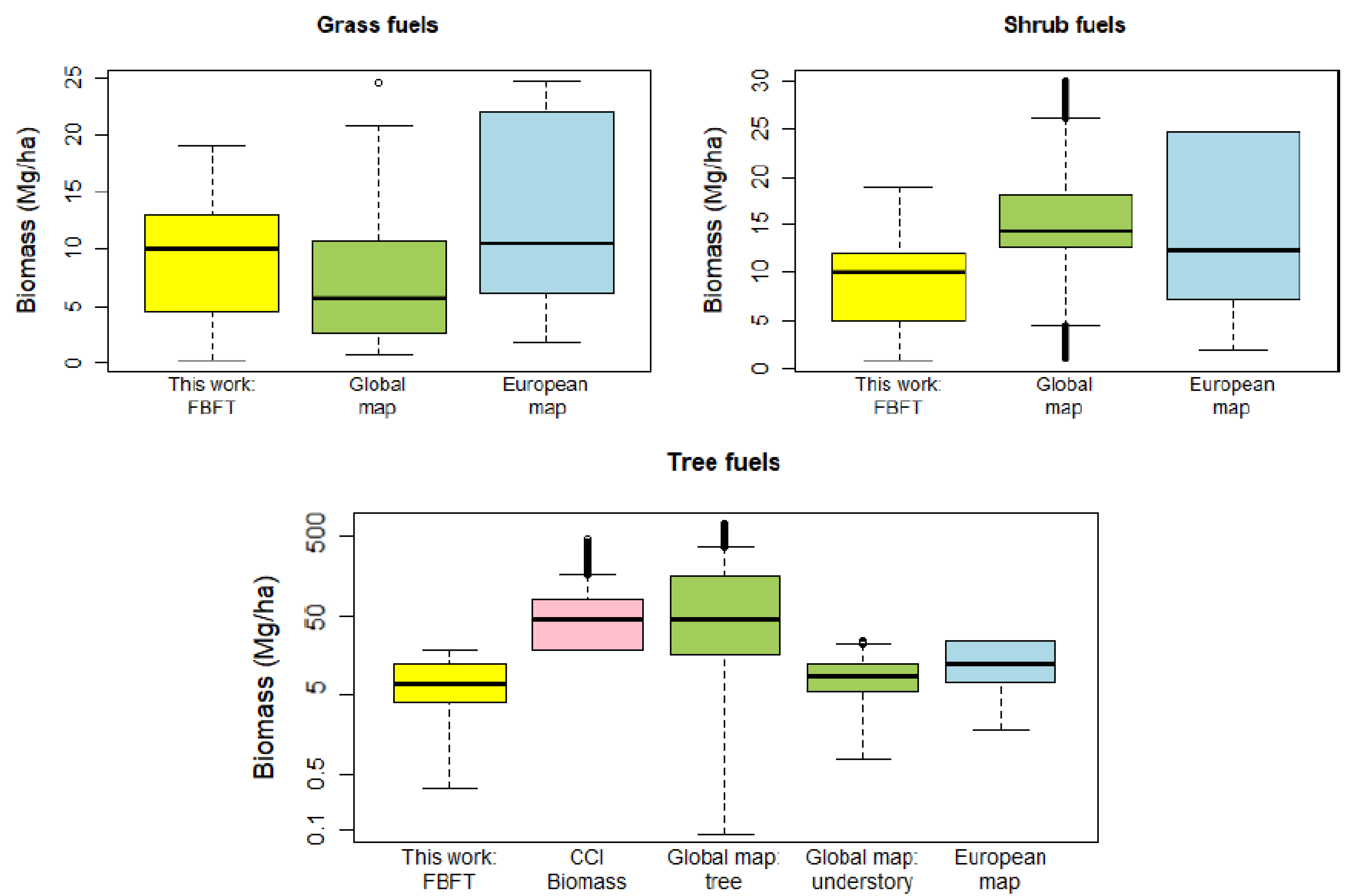
Strict validation of the final FBFT fuel map was not feasible because of the lack of fuel reference data and the practical difficulties of performing alternative field work. Thus, as a first assessment of the final product, we compared our FBFT fuel map with two fuel maps covering the same region: (1) the 2015 global map of Pettinari and Chuvieco [54,91] classified with the Fuel Characteristic Classification System (FCCS), and (2) the European Forest Fire Information System (EFFIS) fuel map classified with NFFL [55]. To enable the comparison of different fuel classification systems, we compared fuel biomass, which is parameterized for each fuel type in FBFT, FCCS, and NFFL. We also compared our results with CCI Biomass values. We performed a statistical analysis: (1) mean and standard deviation of the biomass values for every FBFT-adapted fuel type polygon for the study area, (2) Spearman’s rank correlation, a non-parametric measure to compare the monotonical relation of two variables even if they have a non-linear relationship [92], and (3) box plots. We compared biomass for every fuel type polygon of our FBFT fuel map for the following groups: grass, shrub, and tree fuels.

3. Results

3.1. Vegetation Map

The Support Vector Machine (SVM) vegetation map (Figure 5) shows the study area’s general spatial distribution of vegetation. It shows a wide presence of coniferous species in the northern and eastern mountainous regions of the study area. Evergreen deciduous species dominate in the central and southern regions. Deciduous species predominate in the northern and western regions. Shrubs are represented almost all over the study area, standing out in the eastern region. Grasses have a wide presence in the central and western Iberian Peninsula, mostly associated with agroforestry (dehesa) ecosystems.

The SVM vegetation classification provided an overall accuracy of 85% and kappa 0.81 (

Table A2. Confusion matrix for the vegetation map.

Category	Conif.	Evergr. Broad.	Decid. Broad.	Shr.	Grass.	Other Uses	Total	UA * (%)	CE * (%)
Conif.	35	1	1	1	0	2	39	89.74	10.26
Evergr. broad.	0	36	0	1	3	4	44	81.82	18.18
Decid. broad.	4	2	35	3	0	2	46	76.09	23.91
Shrubs	8	1	0	86	5	19	119	72.27	27.73
Grasses	0	1	0	0	47	9	57	82.46	17.54
Other uses	0	0	0	3	4	288	195	96.41	3.59
Total	48	41	36	95	59	222	500
PA * (%)	74.47	87.80	97.22	90.53	79.67	84.68	Overall accuracy = 85.40%
OE * (%)	25.53	12.2	2.78	9.47	20.33	15.32	Kappa = 0.805

* UA: User accuracy, PA: Producer accuracy, CO: Commission error, OE: Omission error.

in the Appendix A), much higher than the random forest, with an overall accuracy of 56% and kappa 0.44. Thus, we chose the SVM map as the vegetation cartography on which to base the fuel type mapping. The qualitative validation confirms the adjustment of the SVM map to the vegetation patterns observed in the Sentinel-2 images used as reference data. Quantitative validation indicates high agreement between the reference data and the classification.

3.2. Fuel Type Map

The customized Iberian fuel map has 45 fuel types adapted to the study area and input data (Figure 6). Each fuel type is identified by its vegetation type, vegetation horizontal continuity percentage, and biogeographic region.

The five Iberian fuel types with the largest area belong to the Mediterranean region. The largest area belongs to Mediterranean shrubs with 40–70% continuity (83,831 km²), followed by Mediterranean grasses with 70–100% continuity (55,696 km²). These fuel types relate to the arid/semi-arid steppe and the dehesa ecosystems, respectively. No significant differences were observed in means and standard deviations of the vegetation horizontal continuity between biogeographic regions or vegetation types (

Table A3. Characteristics of the Iberian fuel types.

		Vegetation Horizontal Continuity			Area (km2)
		% *	Mean	SD **
Alpine	Conifers	0–40	25.71	9.70	284
		40–70	53.37	7.50	2699
		70–100	71.87	0.87	1
	Evergreen broadleaves	0–40	26.63	8.93	698
		40–70	50.49	7.07	196
		70–100	70.29	0.06	1
	Deciduous broadleaves	0–40	25.43	9.46	662
		40–70	52.08	7.33	1041
		70–100	72.20	0.76	1
	Shrubs	0–40	24.47	11.00	392
		40–70	56.56	8.36	1728
		70–100	73.70	2.82	59
	Grasses	0–40	33.95	3.23	1
		40–70	60.97	5.42	25
		70–100	71.69	1.39	1
Atlantic	Conifers	0–40	25.18	9.81	353
		40–70	55.62	8.72	396
		70–100	71.57	1.29	17
	Evergreen broadleaves	0–40	29.19	8.53	1247
		40–70	53.21	7.74	2266
		70–100	71.70	1.32	28
	Deciduous broadleaves	0–40	26.81	8.67	3798
		40–70	52.45	7.78	25,616
		70–100	71.69	1.31	11
	Shrubs	0–40	31.48	7.15	1911
		40–70	54.56	8.00	7674
		70–100	72.58	2.22	308
	Grasses	0–40	32.15	6.67	724
		40–70	53.23	6.91	7901
		70–100	73.64	2.79	59
Mediterranean	Conifers	0–40	18.21	8.67	36,601
		40–70	51.34	7.08	8934
		70–100	71.33	0.85	3
	Evergreen broadleaves	0–40	17.29	9.58	34,559
		40–70	50.06	6.46	3957
		70–100	71.64	1.16	2
	Deciduous broadleaves	0–40	20.08	10.73	14,248
		40–70	50.72	6.74	4275
		70–100	71.39	1.07	2
	Shrubs	0–40	29.45	9.86	1632
		40–70	60.41	7.70	83,831
		70–100	76.20	4.25	45,459
	Grasses	0–40	32.84	8.95	89
		40–70	61.58	6.96	4139
		70–100	78.20	4.55	55,696

* 40.00% is included in the 0–40% group. 70.00% is included in the 40–70% group. From [78]. ** SD: standard deviation.

in the Appendix A). Fuel types with 0–40% vegetation horizontal continuity presented greater internal variability (highest standard deviation) and therefore greater heterogeneity. Fuel types with 70–100% vegetation horizontal continuity showed less internal variability (lowest standard deviation) and therefore are more homogeneous.

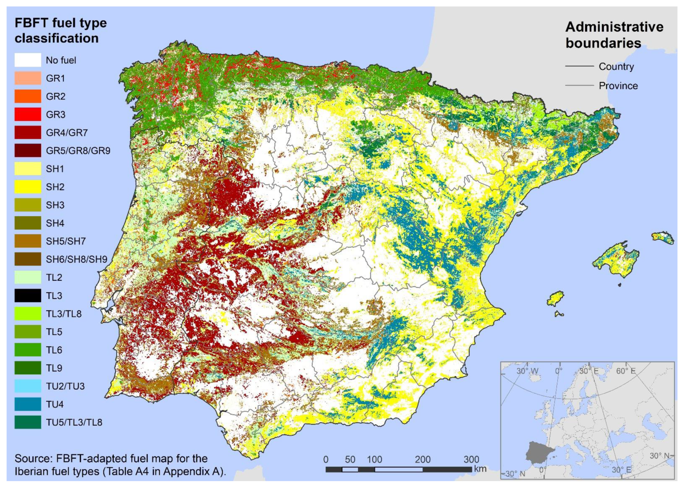
Next, the Iberian fuel types were converted to the FBFT fuel types (see

Table A4. Adaptation of the Iberian fuel types to the FBFT system [21].

			Horizontal Continuity (%) *	FBFT Fuel Type Category
Iberian fuel types	Alpine	Conifers	0–40	TU2/TU3
			40–70	TL3/TL8
			70–100	TL5
		Evergreen broadleaves	0–40	TL2
			40–70	TL6
			70–100	TL9
		Deciduous broadleaves	0–40	TL2
			40–70	TL6
			70–100	TL9
		Shrubs	0–40	SH3
			40–70	SH4
			70–100	SH6/SH8/SH9
		Grasses	0–40	GR1
			40–70	GR3
			70–100	GR5/GR8/GR9
	Atlantic	Conifers	0–40	TU2/TU3
			40–70	TL3/TL8
			70–100	TL5
		Evergreen broadleaves	0–40	TL2
			40–70	TL6
			70–100	TL9
		Deciduous broadleaves	0–40	TL2
			40–70	TL6
			70–100	TL9
		Shrubs	0–40	SH3
			40–70	SH4
			70–100	SH6/SH8/SH9
		Grasses	0–40	GR1
			40–70	GR3
			70–100	GR5/GR8/GR9
	Mediterranean	Conifers	0–40	TU4
			40–70	TU5/TL3/TL8
			70–100	TL5
		Evergreen broadleaves	0–40	TL2
			40–70	TL6
			70–100	TL6
		Deciduous broadleaves	0–40	TL2
			40–70	TL6
			70–100	TL9
		Shrubs	0–40	SH1
			40–70	SH2
			70–100	SH5/SH7
		Grasses	0–40	GR1
			40–70	GR2
			70–100	GR4/GR7

* 40.00% is included in the 0–40% group. 70.00% is included in the 40–70% group. From [78].

in the Appendix A). The FBFT fuel map was generated (Figure 7) with 19 fuel types, and the fuel types were characterized and parameterized (

Table 2. Characterization and parameterization of the FBFT-adapted grass fuel types. The values refer to mean fuel conditions and serve to predict fire behaviour inside and outside the fire season.

FBFT Fuel Type	Brief Fuel type Description	Area (km2)	Mean Biomass (Mg/ha)	Potential Spread Rate	Potential Flame Length
GR1	Short patchy grass, A-SA	814	0.99	M	L
GR2	Moderately coarse continuous grass, A-SA	4139	2.72	H	M
GR3	Very coarse grass, SH-H	7926	3.95	H	M
GR4/GR7	Moderately coarse continuous grass, A-SA	55,696	10.56	VH	VH
GR5/GR8/GR9	Dense, heavy, and very heavy coarse continuous grass, SH-H	59	17.05	VH-E	VH-E

A-SA: arid/semi-arid climate, SH-H: sub-humid/humid climate. VL: very low, L: low, M: moderate, H: high, VH: very high, E: extreme (Table A1 in the Appendix A). Source: original FBFT fuel descriptions [21]. Area has been calculated for the extension occupied by each fuel type for the study area. Note that for non-tree fuels, biomass values are only derived from the original FBFT fuel descriptions [21] and refer to total surface biomass.

,

Table 3. Characterization and parameterization of the FBFT-adapted shrub fuel types. The values refer to mean fuel conditions and serve to predict fire behaviour inside and outside the fire season.

FBFT Fuel Type	Brief Fuel Type Description	Area (km2)	Mean Biomass (Mg/ha)	Potential Spread Rate	Potential Flame Length
SH1	Low shrub fuel load, A-SA	1632	4.20	L	VL
SH2	Moderate shrub fuel load, A-SA	83,831	12.85	L	L
SH3	Moderate heavy shrub load, SH-H	2303	16.43	L	L
SH4	Low to moderate shrub and litter load, SH-H	9402	8.40	H	M
SH5/SH7	Heavy and very heavy shrub load, A-SA	45,459	16.56	VH	VH
SH6/SH8/SH9	Dense shrubs, SH-H	367	19.56	H	H-VH

A-SA: arid/semi-arid climate, SH-H: sub-humid/humid climate. VL: very low, L: low, M: moderate, H: high, VH: very high, E: extreme (Table A1 in the Appendix A). Source: original FBFT fuel descriptions [21]. Area has been calculated for the extension occupied by each fuel type for the study area. Note that for non-tree fuels, biomass values are only derived from the original FBFT fuel descriptions [21] and refer to total surface biomass.

and

Table 4. Characterization and parameterization of the FBFT-adapted tree fuel types (SD: standard deviation). The values refer to mean fuel conditions and serve to predict fire behaviour inside and outside the fire season.

FBFT Fuel Type	Brief Fuel Type Description	Area (km2)	Biomass (Mg/ha)			Potential Spread Rate	Potential Flame Length
			Mean	Mean (CCI Biomass)	SD (CCI Biomass)
TL2	Low broadleaf load	55,211	3.46	36.81	34.23	VL	VL
TL3/TL8	Moderate load conifer litter	3095	7.78	100.78	55.48	VL-M	L
TL5	High load conifer litter	21	2.84	152.15	65.12	L	L
TL6	Moderate broadleaf load	37,353	5.93	95.89	48.22	M	L
TL9	Very high load broadleaf litter	43	16.43	136.03	57.58	M	M
TU2/TU3	Moderate litter load with grass/shrub, SH-H	636	4.94	37.19	34.95	M-H	L-M
TU4	Short conifer trees with grass or moss understory	36,601	16.06	29.07	29.41	M	M
TU5/TL3/TL8	Moderate-high conifer load litter with/without shrub	8934	12.54	95.41	66.55	VL -M	L-M

A-SA: arid/semi-arid climate, SH-H: sub-humid/humid climate. VL: very low, L: low, M: moderate, H: high, VH: very high, E: extreme (Table A1 in the Appendix A). Source: original FBFT fuel descriptions [21], except when the Climate Change Initiative (CCI) Biomass dataset [89] is specified as a source. Area has been calculated for the extension occupied by each fuel type for the study area. Note that for tree fuels, biomass values are derived from the original FBFT fuel descriptions [21], where biomass refers to timber litter and understory biomass; and from the CCI Biomass dataset [89], where biomass refers to Above Ground Biomass (AGB).

). The FBFT fuels’ spatial distribution is similar to that of the customized Iberian fuel map (Figure 6). The fuel types with the largest area Table 2, Table 3 and Table 4) are related to the largest Iberian fuel types (Table A3 and Table A4 in the Appendix A). The fuel type with the largest area (83,831 km²) is SH2, corresponding to Mediterranean shrubs with 40–70% horizontal continuity. The second fuel type with the largest area (55,696 km²) is GR4/GR7, corresponding to Mediterranean grasses with 70–100% horizontal continuity.

The mean biomass of the FBFT-adapted fuel types for the study area (Table 2, Table 3 and Table 4) varies between 1 and 136 Mg/ha, with differences of up to two orders of magnitude between the FBFT-adapted [21] values and the CCI Biomass [89] values. The fuel type with the highest FBFT-adapted mean biomass is SH6/SH8/SH9 (19.56 Mg/ha) followed by GR5/GR8/GR9 (17.05 Mg/ha), corresponding to dense shrubs and grasses from sub-humid/humid climates, respectively. The FBFT-adapted fuel types with the highest mean biomass values extracted from CCI Biomass are TL9 or very high broadleaf litter (136 Mg/ha), and TL5 or high load conifer litter (152 Mg/ha). The more heterogeneous FBFT-adapted fuel types (greater internal variability) are TU5/TL3/TL8 or moderate-high conifer load litter with/without shrub (standard deviation = 66.55), and TL5 or high load conifer litter (standard deviation = 65.12). Non-tree vegetation biomass values could not be extracted from CCI Biomass because this product only indicates tree-vegetation biomass.

The fire potential spread rate and flame length intensity values for surface fires vary between very low and extreme (Table 2, Table 3 and Table 4, Figure 8). A strong visual correlation exists for the spatial distribution of both variables, especially for the arid/semi-arid climate (Mediterranean biogeographic region). The more flammable fuels are moderate-heavy grasses and shrubs (high-extreme fire potential spread ratio and flame length). The highest fire potential spread rates and flame length intensities predominate in the central and western Iberian Peninsula, while the lowest intensity values dominate in the northern and eastern regions of the study area. The GR5/GR8/GR9 fuel type or Alpine and Atlantic highly continuous (70–100%) grasses (56 km²) has the highest values for both variables (very high-extreme).

Finally, grass, shrub, and tree fuels’ biomass was compared with other fuel products (

Table 5. Mean and standard deviation (in parenthesis) biomass (in Mg/ha) of fuel groups (Table A4 in the Appendix A). Spearman’s rank correlation (in brackets) is used to compare this work with other products.

Fuel Group	This Work: FBFT a	CCI Biomass b	Global Fuel Map c	European Fuel Map d
Grass	(T) 8.88 (5.02)	-	(T) 6.99 (5.25) [−0.10] *	(T) 12.59 (7.92) [0.11] *
Shrub	(T) 8.98 (4.95)	-	(SH) 15.11 (6.30) [−0.03] *	(T) 13.70 (7.92) [0.13] *
Tree	(TU) 8.51 (4.89)	(TR) 54.60 (46.21) [−0.17] *	(TR) 122.77 (147.93) [−0.20] * [0.45] ** (U) 9.23 (4.78) [−0.08] * [0.25] **	(TL) 13.84 (7.69) [0.17] * [−0.11] **

^a [21], ^b [89], ^c [54], ^d [55]. Compared with * FBFT [21] and ** CCI Biomass [89] values. Biomass refers to: (T) total surface, (SH) shrub primary, (TU) timber litter and understory, (TR) tree above ground, (U) understory, and (TL) timber litter load. All the correlation values are significant at the 0.01 level (2-tailed).

, Figure 9). This work’s FBFT grass biomass mean is 27% higher compared with the global map [54] and 42% lower compared with the European map [55]. This work’s FBFT shrub biomass mean is 41% and 34% higher compared with the global and European maps, respectively. This work’s FBFT tree biomass mean is 542%, 8%, and 39% lower compared with the CCI Biomass [89] values, the understory biomass of the global map, and the European map, respectively. The derived CCI Biomass tree biomass mean is 56% lower compared with the tree Above Ground Biomass (AGB) of the global map, and 295% higher compared with the European map. The Spearman’s rank correlation values show the highest correlation between this work’s non-tree fuels and the European map (0.11 for grass, and 0.13 for shrub fuels), and between the CCI Biomass values and the tree AGB values of the global map (correlation of 0.45) for the tree fuels. The large differences between biomass values and their distribution for the compared products is due to (1) the different methods used to estimate the biomass values and (2) the dissimilar vegetation parts considered in the biomass estimation.

4. Discussion

The quantitative assessment of the vegetation map presented an overall accuracy of 85% (category errors between 3% and 28%), which is aligned with the goal of 85% global accuracy and no category less than 70% accuracy when classifying land cover with remote sensing [93]. As in [42], the best vegetation map was obtained with SVM versus random forest, possibly due to the small size of our training sample.

The Sentinel-3 Synergy 300 m resolution required some generalization of the vegetation map, ignoring the complexity of the real ecosystems. Thus, mixed pixels were not considered. The vegetation map’s accuracy results could be improved with the optimal search for SVM parameters. The classification was not also performed with Object Based Image Analysis (OBIA), for which other authors obtained similar results to QuickBird and Sentinel-2 (global accuracy 75–90%, categories 50–100%) [43,45] as compared with this work’s Support Vector Machine (SVM) results. Thus, the computational and time costs of OBIA did not seem worth it for the purposes of this work.

The main errors shown in the validation of the vegetation map were caused by Sentinel-3 mixed validation pixels, in which the reflectivity of the different covers was combined. The omission of conifers was mainly related to the confusion with shrubs, mostly in low-density forest areas. Evergreen broadleaves offered commission errors mostly confused with areas of low-density conifers and tall shrubs in agroforestry (dehesas) and mountainous areas. Deciduous broadleaves were confused with conifers in mixed forest areas in the northern and western forests. The shrubs’ commission errors were mainly related to confusion with permanent crops (vineyards, fruit trees). The shrubs’ omission errors were associated with their confusion with annual crops and mixed pixels of shrubs and grasses. Omission and commission errors for grasses were mainly related to patchy grass areas.

Regarding the conversion from the customized Iberian fuel map to the FBFT fuel map, several problems were found. For instance, this work assumes an equivalence between the United States FBFT sub-humid/humid climate and the Atlantic and Alpine European biogeographic regions, as well as between the United States FBFT arid/semi-arid climate and the Mediterranean European biogeographic region. Moreover, the Atlantic and Alpine fuel types were impossible to separate in the FBFT system [21]. This issue could be improved for the European FBFT fuel map by complementing the information of the FBFT fuel types with the biogeographic region in which they are included. For this, every European-adapted FBFT fuel type could be split into as many fuel types as European biogeographic regions it belongs to.

Some difficulties were also found concerning the broadleaves because the FBFT system does not distinguish between evergreen and deciduous broadleaves. Thus, we adapted the broadleaves based on the biogeographic region, horizontal continuity, and fuel load. Therefore, caution should be taken when using the FBFT fuel map for these vegetation categories. The Iberian and FBFT fuel maps have a similar general spatial distribution of fuels because one is based on the other. The fuel types with the largest area are the Mediterranean types because this is the largest biogeographic region in the study area.

Moreover, in this work we have used the original FBFT descriptions and visual analysis of the United States FBFT fuel map [88] to convert from the Iberian fuel types to the standard FBFT fuel types (Table A4 in the Appendix A). A way to improve this in future works would be to compare the quantitative environmental specifications (such as rainfall, temperature, evapotranspiration, available water, and drought index) for the United States FBFT fuel types and the Iberian fuel types. This could be done by comparing these metrics for the United States, Spain, and Portugal.

Concerning the fuel type parameters, the tree fuels’ biomass values derived from CCI Biomass [89] presented great differences (up to two orders of magnitude) from those extracted from the FBFT system [21]. The reason for this is that for the tree fuel types, the CCI Biomass values refer to total AGB and the FBFT values to timber litter and understory biomass. Moreover, CCI Biomass values offer pixel-disaggregated information compared with the FBFT values, for which the mean biomass values of the fuel types are assigned to all the extension occupied by an FBFT fuel type. Biomass data are expected to improve with the upcoming ESA Biomass mission in 2022 [16].

Dense grasslands and shrubs are the most flammable fuel types [94]. This agrees with the obtained results, which show that the GR5/GR8/GR9 fuel type or Alpine and Atlantic highly continuous (70–100%) grasses entails the highest fire risk and danger: very high-extreme fire potential spread rate and flame length. Also, grasses and shrubs occupy much of the surface of the study area. Thus, the biggest economic and human fire prevention efforts should be focused here.

In terms of intercomparison with existing vegetation and fuel maps of the study area, a strict validation was not possible, since the scales, methods, and classification schemes change between products. Still, the vegetation map’s distribution agrees with that detailed for the study area [63,77], and its classification scheme is similar to that defined on larger scales with Sentinel-2 [43,50]. Also, the global [54,91] and the European [55] fuel maps have, respectively, 41 and 10 fuel types for the study area, while here we mapped 45 (Iberian fuel map) and 19 (FBFT fuel map) types. This difference may be caused by the use of the vegetation horizontal continuity to develop fuel types in this work, while in [54] it is only used to parameterize and the FBFT system uses field measures and photo series.

Furthermore, this work’s comparison with the global [54] and European [55] fuel maps shows some similarities for the mean biomass values but does not show very strong associations for the distribution of values, probably caused by the dissimilar biomass estimation methods. FBFT is based on field measures and photo series, and for tree fuels describes timber litter and understory [21]; CCI Biomass is derived from RADAR images and indicates tree AGB [90]; FCCS (global map) infers vegetation parts’ biomass from expert opinion, scientific literature, photo series, and pre-existing databases [95]; NFFL (European map) is based on observations and for tree fuels describes only timber litter [35]. Thus, the biomass values differ between products. This may explain the high tree mean biomass differences when compared with other mean biomass values. However, it is important to note that there is no reason why the global and European fuel maps should be considered more accurate than this work’s result. A homogeneous field sampling for the fuel parameters in the study area would be useful for a strict validation of this work’s fuel maps. Moreover, CCI Biomass indicates AGB while FBFT, FCCS (except for the tree Above Ground Biomass parameter), and NFFL describe surface fuel biomass affecting surface fires. Hence, the fuel parameterization methods and assumptions, usually determined by the fuel categories of the standard fuel classification systems, stand out as a key aspect to homogenize fire risk assessment, evidencing the importance of an integrated fuel mapping strategy across regions.

The final fuel descriptions and maps are influenced by the errors of their inputs. For the FBFT fuel map, adaptation-derived errors also had an effect. In addition, the original FBFT system uses field measures and photo series to describe the fuel types, which results in dissimilar fuel descriptions and difficult adaptation. Thus, the main limitations of this work are (1) the selected inputs, which limit the disaggregation of fuel types, (2) the errors of the inputs and the generated vegetation map, which influence the final map’s accuracy, and (3) the FBFT adaptation difficulties. These aspects limit the utility of the final fuel map for local studies. It is also limiting not to consider mixed categories and pixels.

The main contribution of our methodology was to derive an easily upgradeable and reproducible method to map fuel types and estimate fire propagation potential to improve fire risk assessment. It is expected to be applicable to regional, continental, or global scales, adapting the methods and data if necessary. Sentinel-3 Synergy images offer an advantage over higher resolution sensors, which would require a greater computational effort for regional-continental fuel mapping. The standard FBFT fuel types facilitate the homogenization of fuel maps across regions. Our methodology is expected to be useful for fuel mapping that can be updated for short time periods (semi-annual or annual), usable in fire simulation models to consider the fuels’ high temporal variability in fire risk assessment. It serves to optimize the prevention, resource allocation, and management of wildland fires. This work is relevant because it generates the framework for an updated large-scale (European) fuel mapping.

Future works should focus on refining the fuel type maps by subdividing categories, searching for optimal SVM parameters for the vegetation classification, considering mixed vegetation categories and vegetation vertical characteristics (using LiDAR data), and comparing with classifiers such as OBIA. Future works should also make efforts to compare the results with fieldwork or local products. Regarding this, it would be useful to develop a European database with homogeneous field sampling to help validation and selection of remote sensing products in future works concerning vegetation and fuel mapping, and fuel parameterization.

5. Conclusions

This work generated an FBFT [21] fuel map for the Iberian Peninsula and the Balearic Islands with 19 fuel types, which were also parameterized. Estimated fire behaviour (potential spread rate and flame length) was also mapped. The input data were Sentinel-3 Synergy images, MODIS vegetation continuous field collection 6 maps, a map of biogeographic regions, and the CCI Biomass map. Intercomparison of the final FBFT fuel map with other fuel products showed some agreement for mean biomass values but did not present a strong correlation between products in the distribution of values. As intermediate results, this work generated a vegetation map and a map of 45 customized fuel types, and proposed an adaptation to the FBFT system [21] for the study area.

Up-to-date mapping of fuel types is essential for wildland fire prevention. This work has wide applicability because it proposes a methodology to develop an easily upgradeable fuel cartography on a regional-continental scale for wildland fire risk assessment. This is a priority future line of research because it will facilitate, speed up, and optimize wise decision-making. The proposed methodology can be used to classify fuel types in other regions, adapting the fuel categories if necessary. The next step should be to apply this methodology to homogenize fuel maps in the European Union, a vital point to derive an integrated fire risk strategy adapted to European conditions, which is a key objective of the FirEUrisk project, in which our present research fits.

References

- Archibald, S.; Lehmann, C.E.R.; Belcher, C.M.; Bond, W.J.; Bradstock, R.A.; Daniau, A.L.; Dexter, K.G.; Forrestel, E.J.; Greve, M.; He, T.; et al. Biological and geophysical feedbacks with fire in the Earth system. Environ. Res. Lett. 2018, 13, 033003. [Google Scholar] [CrossRef] [Green Version]
- Koutsias, N.; Karteris, M. Classification analyses of vegetation for delineating forest fire fuel complexes in a Mediterranean test site using satellite remote sensing and GIS. Int. J. Remote Sens. 2003, 24, 3093–3104. [Google Scholar] [CrossRef]
- Pausas, J.G.; Keeley, J.E. A burning story: The role of fire in the history of life. BioScience 2009, 59, 593–601. [Google Scholar] [CrossRef] [Green Version]
- Eva, H.; Lambin, E.F. Fires and land-cover change in the tropics: A remote sensing analysis at the landscape scale. J. Biogeogr. 2000, 27, 765–776. [Google Scholar] [CrossRef]
- Cano-Crespo, A.; Oliveira, P.J.C.; Boit, A.; Cardoso, M.; Thonicke, K. Forest edge burning in the Brazilian Amazon promoted by escaping fires from managed pastures. J. Geophys. Res. Biogeosci. 2015, 120, 2095–2107. [Google Scholar] [CrossRef] [Green Version]
- McCaffrey, S. Thinking of wildfire as a natural hazard. Soc. Nat. Resour. 2004, 17, 509–516. [Google Scholar] [CrossRef]
- Bowman, D.M.J.S.; Balch, J.; Artaxo, P.; Bond, W.J.; Cochrane, M.A.; D’Antonio, C.M.; De Fries, R.; Johnston, F.H.; Keeley, J.E.; Krawchuk, M.A.; et al. The human dimension of fire regimes on Earth. J. Biogeogr. 2011, 38, 2223–2236. [Google Scholar] [CrossRef] [Green Version]
- Knorr, W.; Arneth, A.; Jiang, L. Demographic controls of future global fire risk. Nat. Clim. Chang. 2016, 6, 781–785. [Google Scholar] [CrossRef]
- Giglio, L.; Boschetti, L.; Roy, D.P.; Humber, M.L.; Justice, C.O. The Collection 6 MODIS burned area mapping algorithm and product. Remote Sens. Environ. 2018, 217, 72–85. [Google Scholar] [CrossRef] [PubMed]
- Lizundia-Loiola, J.; Otón, G.; Ramo, R.; Chuvieco, E. A spatio-temporal active-fire clustering approach for global burned area mapping at 250 m from MODIS data. Remote Sens. Environ. 2020, 236, 1–18. [Google Scholar] [CrossRef]
- Kalabokidis, K.; Palaiologou, P.; Gerasopoulos, E.; Giannakopoulos, C.; Kostopoulou, E.; Zerefos, C. Effect of Climate Change Projections on Forest Fire Behaviour and Values-at-Risk in Southwestern Greece. Forests 2015, 6, 2214–2240. [Google Scholar] [CrossRef] [Green Version]
- De Rigo, D.; Libertà, G.; Durrant, T.H.; Vivancos, A.; San-Miguel-Ayanz, J. Forest Fire Danger Extremes in Europe under Climate Change: Variability and Uncertainty; Publications Office of the European Union: Luxembourg, 2017. [CrossRef]
- Moreira, F.; Viedma, O.; Arianoutsou, M.; Curt, T.; Koutsias, N.; Rigolot, E.; Barbati, A.; Corona, P.; Vaz, P.; Xanthopoulos, G.; et al. Landscape—Wildfire interactions in southern Europe: Implications for landscape management. J. Environ. Manag. 2011, 92, 2389–2402. [Google Scholar] [CrossRef] [PubMed] [Green Version]
- Moritz, M.A.; Parisien, M.; Batllori, E.; Krawchuk, M.A.; Van Dorn, J.; Ganz, D.J.; Hayhoe, K. Climate change and disruptions to global fire activity. Ecosphere 2012, 3, 1–22. [Google Scholar] [CrossRef]
- San-Miguel-Ayanz, J.; Moreno, J.M.; Camia, A. Analysis of large fires in European Mediterranean landscapes: Lessons learned and perspectives. For. Ecol. Manag. 2013, 294, 11–22. [Google Scholar] [CrossRef]
- Pettinari, M.L.; Chuvieco, E. Fire Danger Observed from Space. Surv. Geophys. 2020, 41, 1437–1459. [Google Scholar] [CrossRef]
- Pyne, S.J. Introduction to Wildland Fire: Fire Management in the United States; John Wiley & Sons: New York, NY, USA, 1984. [Google Scholar]
- Chuvieco, E.; Cocero, D.; Riaño, D.; Martin, P.; Martínez-Vega, J.; De La Riva, J.; Pérez, F. Combining NDVI and surface temperature for the estimation of live fuel moisture content in forest fire danger rating. Remote Sens. Environ. 2004, 92, 322–331. [Google Scholar] [CrossRef]
- Marino, E.; Ranz, P.; Tomé, J.L.; Noriega, M.A.; Esteban, J.; Madrigal, J. Generation of high-resolution fuel model maps from discrete airborne laser scanner and Landsat-8 OLI: A low-cost and highly updated methodology for large areas. Remote Sens. Environ. 2016, 187, 267–280. [Google Scholar] [CrossRef]
- Chuvieco, E.; Riaño, D.; Van Wagtendok, J.; Morsdof, F. Fuel Loads and Fuel Type Mapping. In Wildland Fire Danger: Estimation and Mapping: The Role of Remote Sensing Data; Chuvieco, E., Ed.; World Scientific Publishing Co. Ltd.: Singapore, 2003; pp. 119–142. [Google Scholar]
- Scott, J.; Burgan, R. Standard Fire Behaviour Fuel Models: A Comprehensive Set for Use with Rothermel’s Surface Fire Spread Model; Rocky Mountain Research Station; US Department of Agriculture, Forest Service, Rocky Mountain Research Station: Washington, DC, USA, 2005.
- Ottmar, R.D.; Alvarado, E. Linking vegetation patterns to potential smoke production and fire hazard. In Proceedings of the Sierra Nevada Science Symposium, Kings Beach, CA, USA, 7–10 October 2002. [Google Scholar]
- Chuvieco, E.; Van Wagtendonk, J.W.; Riaño, D.; Yebra, M.; Wagtendonk, J.; Riaffo, D.; Yebra, I.; Ustin, S.L. Estimation of Fuel Conditions for Fire Danger Assessment. In Earth Observation of Wildland Fires in Mediterranean Ecosystems; Chuvieco, E., Ed.; Springer: Dordrecht, The Netherlands, 2009; pp. 83–96. [Google Scholar]
- Arroyo, L.A.; Pascual, C.; Manzanera, J.A. Fire models and methods to map fuel types: The role of remote sensing. For. Ecol. Manag. 2008, 256, 1239–1252. [Google Scholar] [CrossRef] [Green Version]
- Burgan, R.E.; Klaver, R.W.; Klarer, J.M. Fuel models and fire potential from satellite and surface observation. Int. J. Wildland Fire 1998, 8, 159–170. [Google Scholar] [CrossRef]
- Dymond, C.C.; Roswintiarti, O.; Brady, M. Characterizing and mapping fuels for Malaysia and western Indonesia. Int. J. Wildland Fire 2004, 13, 323–334. [Google Scholar] [CrossRef]
- Lasaponara, R.; Lanorte, A. Remotely sensed characterization of forest fuel types by using satellite ASTER data. Int. J. Appl. Earth Obs. Geoinf. 2007, 9, 225–234. [Google Scholar] [CrossRef]
- Eftychidis, G.; Laneve, G.; Ferrucci, F.; Sebastian Lopez, A.; Lourenco, L.; Clandillon, S.; Tampellini, L.; Hirn, B.; Diagourtas, D.; Leventakis, G. PREFER: A European service providing forest fire management support products. In Proceedings of the SPIE 9535, Third International Conference on Remote Sensing and Geoinformation of the Environment (RSCy2015), Paphos, Cyprus, 16–19 March 2015. [Google Scholar] [CrossRef]
- Anderson, H. Aids to Determining Fuel Models for Estimating Fire Behaviour; US Department of Agriculture, Forest Service, Intermountain Forest and Range Experiment Station: Washington, DC, USA, 1982.
- Forestry Canada Fire Danger Group. Development and Structure of the Canadian Fire Behaviour Prediction System; Information Report ST-X-3; Forestry Canada: Ottawa, ON, Canada, 1992.
- Riaño, D.; Chuvieco, E.; Salas, J.; Palacios-Orueta, A.; Bastarrika, A. Generation of fuel type maps from Landsat TM images and ancillary data in Mediterranean ecosystems. Can. J. For. Res. 2002, 32, 1301–1315. [Google Scholar] [CrossRef]
- Alonso-Benito, A.; Arroyo, L.A.; Arbelo, M.; Hernández-Leal, P.; González-Calvo, A. Pixel and object-based classification approaches for mapping forest fuel types in Tenerife Island from ASTER data. Int. J. Wildland Fire 2013, 22, 306–317. [Google Scholar] [CrossRef]
- Palaiologou, P.; Kalabokidis, K.; Kyriakidis, P. Forest mapping by geoinformatics for landscape fire behaviour modelling in coastal forests, Greece. Int. J. Remote Sens. 2013, 34, 4466–4490. [Google Scholar] [CrossRef]
- Rothermel, R. How to Predict the Spread and Intensity of Forest and Range Fires; National Wildfire Coordinating Group, USDA Forest Service Intermountain Research Station: Boise, ID, USA, 1983.
- Albini, F. Estimating Wildfire Behaviour and Effects; General Technical Report INT-30; USDA Forest Service, Intermountain Forest and Range Experiment Station: Odgen, UT, USA, 1976.
- Chuvieco, E.; Aguado, I.; Salas, J.; García, M.; Yebra, M.; Oliva, P. Satellite Remote Sensing Contributions to Wildland Fire Science and Management. Curr. For. Rep. 2020, 6, 81–96. [Google Scholar] [CrossRef]
- Gale, M.G.; Cary, G.J.; Van Dijk, A.I.J.M.; Yebra, M. Forest fire fuel through the lens of remote sensing: Review of approaches, challenges and future directions in the remote sensing of biotic determinants of fire behaviour. Remote Sens. Environ. 2021, 255. [Google Scholar] [CrossRef]
- García, M.; Popescu, S.; Riaño, D.; Zhao, K.; Neuenschwander, A.; Agca, M.; Chuvieco, E. Characterization of canopy fuels using ICESat/GLAS data. Remote Sens. Environ. 2012, 123, 81–89. [Google Scholar] [CrossRef]
- Mallinis, G.; Mitsopoulos, I.D.; Dimitrakopoulos, A.P.; Gitas, I.Z.; Karteris, M. Local-scale fuel-type mapping and fire behaviour prediction by employing high-resolution satellite imagery. IEEE J. Sel. Top. Appl. Earth. Obs. Remote Sens. 2008, 1, 230–239. [Google Scholar] [CrossRef]
- Salas, J.; Chuvieco, E. Aplicación de imágenes Landsat-TM a la cartografía de modelos combustibles. Rev. Teledetec. 1995, 5, 1–12. [Google Scholar]
- Castro, R.; Chuvieco, E. Modeling Forest fire danger from geographic information systems. Geocarto Int. 1998, 13, 15–23. [Google Scholar] [CrossRef]
- Domingo, D.; de la Riva, J.; Lamelas, M.T.; García-Martín, A.; Ibarra, P.; Echeverría, M.; Hoffrén, R. Fuel Type Classification Using Airborne Laser Scanning and Sentinel 2 Data in Mediterranean Forest Affected by Wildfires. Remote Sens. 2020, 12, 3660. [Google Scholar] [CrossRef]
- Stefanidou, A.; Gitas, I.Z.; Katagis, T. A national fuel type mapping method improvement using sentinel-2 satellite data. Geocarto Int. 2020, 1, 1–21. [Google Scholar] [CrossRef]
- Marino, E.; Yebra, M.; Guillén-Climent, M.; Algeet, N.; Tomé, J.L.; Madrigal, J.; Guijarro, M.; Hernando, C. Investigating live fuel moisture content estimation in fire-prone shrubland from remote sensing using empirical modelling and RTM simulations. Remote Sens. 2020, 12, 2251. [Google Scholar] [CrossRef]
- Arroyo, L.A.; Healey, S.P.; Cohen, W.B.; Cocero, D.; Manzanera, J.A. Using object-oriented classification and high-resolution imagery to map fuel types in a Mediterranean region. J. Geophys. Res. Biogeosci. 2006, 111, 1–10. [Google Scholar] [CrossRef] [Green Version]
- Mutlu, M.; Popescu, S.C.; Stripling, C.; Spencer, T. Mapping surface fuel models using lidar and multispectral data fusion for fire behaviour. Remote Sens. Environ. 2008, 112, 274–285. [Google Scholar] [CrossRef]
- Alonso-Benito, A.; Arroyo, L.A.; Arbelo, M.; Lorenzo-Gil, A.; Hernández-Leal, P.; Núñez, L. Cartografiado de modelos de combustible mediante la Fusión de Imágenes WorldView-2 y datos LiDAR. Un caso de estudio en la isla de Tenerife. In Proceedings of the XV Simposio Internacional, Cayenne, France, 19–23 November 2021. [Google Scholar]
- Alonso-Benito, A.; Arroyo, L.A.; Arbelo, M.; Hernández-Leal, P. Fusion of WorldView-2 and LiDAR data to map fuel types in the Canary Islands. Remote Sens. 2016, 8, 669. [Google Scholar] [CrossRef] [Green Version]
- Bright, B.C.; Hudak, A.T.; Meddens, A.J.; Hawbaker, T.J.; Briggs, J.S.; Kennedy, R.E. Prediction of Forest Canopy and Surface Fuels from Lidar and Satellite Time Series Data in a Bark Beetle-Affected Forest. Forests 2017, 8, 322. [Google Scholar] [CrossRef] [Green Version]
- García, M.; Saatchi, S.; Casas, A.; Koltunov, A.; Ustin, S.; Ramirez, C.; Balzter, H. Extrapolating Forest Canopy Fuel Properties in the California Rim Fire by Combining Airborne LiDAR and Landsat OLI Data. Remote Sens. 2017, 9, 394. [Google Scholar] [CrossRef] [Green Version]
- Immitzer, M.; Neuwirth, M.; Böck, S.; Brenner, H.; Vuolo, F.; Atzberger, C. Optimal Input Features for Tree Species Classification in Central Europe Based on Multi-Temporal Sentinel-2 Data. Remote Sens. 2019, 11, 2599. [Google Scholar] [CrossRef] [Green Version]
- Pettinari, M.L.; Ottmar, R.D.; Prichard, S.J.; Andreu, A.G.; Chuvieco, E. Development and mapping of fuel characteristics and associated fire potentials for South America. Int. J. Wildland Fire 2014, 23, 643–654. [Google Scholar] [CrossRef]
- Pettinari, M.L.; Chuvieco, E. Cartografía de combustible y potenciales de incendio en el continente Africano utilizando FCCS. Rev. Teledetec. 2015, 2015, 1–10. [Google Scholar] [CrossRef] [Green Version]
- Pettinari, M.L.; Chuvieco, E. Generation of a global fuel data set using the Fuel Characteristic Classification System. Biogeosciences 2016, 13, 2061–2076. [Google Scholar] [CrossRef] [Green Version]
- EFFIS Data and Services. EFFIS Fuel Map. 2000. Available online: https://effis.jrc.ec.europa.eu/applications/data-and-services (accessed on 21 May 2021).
- Cardoso-Castro-Rego, F.; Moreno-Rodríguez, J.M.; Vallejo-Calzada, V.R.; Xanthopoulos, G. Forest Fires—Sparking Firesmart Policies in the EU. Research & Innovation Projects for Policy; Faivre, N., Ed.; Publications Office of the European Union: Luxembourg, 2018.
- San-Miguel-Ayanz, J.; Rodrigues, M.; de Oliveira, S.S.; Pacheco, C.K.; Moreira, F.; Duguy, B.; Camia, A. Land Cover Change and Fire Regime in the European Mediterranean Region. In Post-Fire Management and Restoration of Southern European Fores; San-Miguel-Ayanz, J., Rodrigues, M., de Oliveira, S.S., Pacheco, C.K., Moreira, F., Duguy, B., Camia, A., Eds.; Springer: Dordrecht, The Netherlands, 2012; pp. 21–43. [Google Scholar]
- San-Miguel-Ayanz, J.; Durrant, T.; Boca, R.; Maianti, P.; Libertà, G.; Artes Vivancos, T.; Jacome Felix Oom, D.; Branco, A.; De Rigo, D.; Ferrari, D.; et al. Forest Fires in Europe, Middle East and North Africa 2019; Publications Office of the European Union: Luxembourg, 2020.
- Oliveira, S.; Oehler, F.; San-Miguel-Ayanz, J.; Camia, A.; Pereira, J.M.C. Modeling spatial patterns of fire occurrence in Mediterranean Europe using Multiple Regression and Random Forest. For. Ecol. Manag. 2012, 275, 117–129. [Google Scholar] [CrossRef]
- European Environment Agency. Biogeographical Regions. 2016. Available online: https://www.eea.europa.eu/data-and-maps/data/biogeographical-regions-europe-3 (accessed on 12 May 2021).
- EFFIS Data and Services. Download Real-Time updated Burnt Areas Database. 2021. Available online: https://effis.jrc.ec.europa.eu/applications/data-and-services (accessed on 21 May 2021).
- Trigo, R.M.; Sousa, P.M.; Pereira, M.G.; Rasilla, D.; Gouveia, C.M. Modelling wildfire activity in Iberia with different atmospheric circulation weather types. Int. J. Climatol. 2013, 36, 2761–2778. [Google Scholar] [CrossRef]
- Loidi, J. The Vegetation of the Iberian Peninsula; Springer: Utrecht, The Netherlands, 2017. [Google Scholar]
- Sentinel-3: Visión Panorámica Para Copérnico. Available online: https://www.esa.int/Space_in_Member_States/Spain/Sentinel-3_Vision_panoramica_para_Copernico (accessed on 5 April 2021).
- Sentinel-3 Synergy Introduction. Available online: https://sentinel.esa.int/web/sentinel/user-guides/sentinel-3-synergy (accessed on 17 April 2021).
- Wooster, M.J.; Xu, W.; Nightingale, T. Sentinel-3 SLSTR active fire detection and FRP product: Pre-launch algorithm development and performance evaluation using MODIS and ASTER datasets. Remote Sens. Environ. 2012, 120, 236–254. [Google Scholar] [CrossRef]
- Xu, W.; Wooster, M.J.; Polehampton, E.; Yemelyanova, R.; Zhang, T. Sentinel-3 active fire detection and FRP product performance-Impact of scan angle and SLSTR middle infrared channel selection. Remote Sens. Environ. 2021, 261, 112460. [Google Scholar] [CrossRef]
- Sørensen, K. Implementing an Ensemble Convolutional Neural Network on Sentinel-1 Synthetic Aperture Radar data and Sentinel-3 Radio-Metric Data for the Detecting of Forest Fires; Technical University of Denmark: Kongens Lyngby, Denmark, 2020. [Google Scholar]
- Rashkovetsky, D.; Mauracher, F.; Langer, M.; Schmitt, M. Wildfire Detection from Multisensor Satellite Imagery Using Deep Semantic Segmentation. IEEE J. Sel. Top. Appl. Earth. Obs. Remote. Sens. 2021, 14, 7001–7016. [Google Scholar] [CrossRef]
- Lizundia-Loiola, J.; Pettinari, M.L.; Chuvieco, E. ESA CCI ECV Fire Disturbance: D2.1.2 Algorithm Theoretical Basis Document (ATBD)—Sentinel-3, Version 1.1. 2020. Available online: https://www.esa-fire-cci.org/documents (accessed on 2 August 2021).
- Copernicus Open Access Hub. Available online: https://scihub.copernicus.eu/dhus/#/home (accessed on 25 April 2021).
- Lydersen, J.M.; Collins, B.M.; Knapp, E.E.; Roller, G.B.; Stephens, S. Relating fuel loads to overstorey structure and composition in a fire-excluded Sierra Nevada mixed conifer forest. Int. J. Wildland Fire 2015, 24, 484–494. [Google Scholar] [CrossRef]
- Huete, A.R. A soil-adjusted vegetation index (SAVI). Remote Sens. Environ. 1988, 25, 295–309. [Google Scholar] [CrossRef]
- Huete, A.R.; Justice, C.; Liu, H. Development of vegetation and soil indices for MODIS-EOS. Remote Sens. Environ. 1994, 49, 224–234. [Google Scholar] [CrossRef]
- Gao, B.C. NDWI—A normalized difference water index for remote sensing of vegetation liquid water from space. Remote Sens. Environ. 1996, 58, 257–266. [Google Scholar] [CrossRef]
- Mountrakis, G.; Im, J.; Ogole, C. Support vector machines in remote sensing: A review. ISPRS J. Photogramm. 2011, 66, 247–259. [Google Scholar] [CrossRef]
- Julien, Y.; Sobrino, J.A.; Mattar, C.; Ruescas, A.B.; Jiménez-Muñoz, J.C.; Sòria, G.; Hidalgo, V.; Atitar, M.; Franch, B.; Cuenca, J. Temporal analysis of normalized difference vegetation index (NDVI) and land surface temperature (LST) parameters to detect changes in the Iberian land cover between 1981 and 2001. Int. J. Remote Sens. 2011, 32, 2057–2068. [Google Scholar] [CrossRef]
- DiMiceli, C.M.; Carrol, M.L.; Sohlberg, R.A.; Huang, C.; Hansen, M.C.; Townsend, J.R.G. MOD44B MODIS/Terra Vegetation Continuous Fields Yearly L3 Global 250 m SIN Grid V006. Available online: https://lpdaac.usgs.gov/products/mod44bv006/ (accessed on 6 September 2021).
- Townshed, J. User Guide for the MODIS Vegetation Continuous Fields Product Collection 6 Version 1; Universiy of Maryland: College Park, MD, USA, 2017. [Google Scholar]
- Barthlott, W.; Hostert, A.; Kier, G.; Küper, W.; Kreft, H.; Mutke, J.; Rafiqpoor, M.D.; Sommer, J.H. Geographic patterns of vascular plant diversity at continental to global scales. Erdkunde 2007, 61, 305–316. [Google Scholar] [CrossRef]
- Kreft, H.; Jetz, W. Global patterns and determinants of vascular plant diversity. Proc. Natl. Acad. Sci. USA 2007, 104, 5925–5930. [Google Scholar] [CrossRef] [Green Version]
- Saatchi, S.S.; Harris, N.L.; Brown, S.; Lefsky, M.A.; Mitchard, E.T.A.; Salas, W.; Zutta, B.R.; Buermann, W.; Lewis, S.L.; Hagen, S.; et al. Benchmark map of forest carbon stocks in tropical regions across three continents. Proc. Natl. Acad. Sci. USA 2011, 108, 9899–9904. [Google Scholar] [CrossRef] [Green Version]
- Baccini, A.; Goetz, S.J.; Walker, W.S.; Laporte, N.T.; Sun, M.; Sulla-Menashe, D.; Hackler, J.; Beck, P.S.A.; Dubayah, R.; Friedl, M.A.; et al. Estimated carbon dioxide emissions from tropical deforestation improved by carbon-density maps. Nat. Clim. Chang. 2012, 2, 182–185. [Google Scholar] [CrossRef]
- Banin, L.; Lewis, S.L.; Lopez-Gonzalez, G.; Baker, T.R.; Quesada, C.A.; Chao, K.-J.; Burslem, D.F.R.P.; Nilus, R.; Abu Salim, K.; Keeling, H.C.; et al. Tropical forest wood production: A cross-continental comparison. J. Ecol. 2014, 102, 1025–1037. [Google Scholar] [CrossRef] [Green Version]
- Thurner, M.; Beer, C.; Santoro, M.; Carvalhais, N.; Wutzler, T.; Schepaschenko, D.; Shvidenko, A.; Kompter, E.; Ahrens, B.; Levick, S.R.; et al. Carbon stock and density of northern boreal temperate forests. Global Ecol. Biogeogr. 2014, 23, 297–310. [Google Scholar] [CrossRef]
- Lehmann, C.E.R.; Anderson, M.T.; Sankaran, M.; Higgins, S.I.; Archibald, S.; Hoffman, W.A.; Hanan, N.P.; Williams, R.J.; Fensham, R.J.; Felfili, J.; et al. Savanna vegetation-fire-climate relationships differ among continents. Science 2014, 343, 548–552. [Google Scholar] [CrossRef] [PubMed]
- Rogers, B.M.; Soja, A.J.; Goulden, M.L.; Randerson, J.T. Influence of tree species on continental differences in boreal fires and climate feedback. Nat. Geosci. 2015, 8, 228–234. [Google Scholar] [CrossRef]
- U.S. Department of the Interior. 40 Scott and Burgan Fire Behavior Fuel Models. 2012. Available online: https://landfire.gov/fbfm40.php (accessed on 26 May 2021).
- Santoro, M.; Cartus, O. ESA Biomass Climate Change Initiative (Biomass cci): Global Datasets of Forest Above-Ground Biomass for the Years 2010, 2017 and 2018, v2. Centre for Environmental Data Analysis, 2021. Available online: https://catalogue.ceda.ac.uk/uuid/84403d09cef3485883158f4df2989b0c (accessed on 7 June 2021).
- Santoro, M.; Quegan, S. CCI Biomass Product User Guide Year 2, Version 2.0; ESA Climate Change Initiative—Biomass Project 2020; Aberystwyth University and Gamma Remote Sensing: Wales, UK, 2018. [Google Scholar]
- Pettinari, M.L. Global Fuelbed Dataset; Department of Geology, Geography and Environment, University of Alcala: Alcala, Spain, 2015; Available online: https://doi.pangaea.de/10.1594/PANGAEA.84980 (accessed on 15 May 2021).
- Zar, J.H. Spearman rank correlation. In Encyclopedia of Biostatistics; Armitage, P., Colton, T., Eds.; John Wiley and Sons: Chichester, UK, 2005. [Google Scholar]
- Thomlinson, J.R.; Bolstad, P.V.; Cohen, W.B. Coordinating methodologies for scaling landcover classifications from site-specific to global: Steps toward validating global map products. Remote Sens. Environ. 1999, 70, 16–28. [Google Scholar] [CrossRef]
- Pettinari, M.L.; Chuvieco, E. Fire behaviour simulation from global fuel and climatic information. Forests 2017, 8, 179. [Google Scholar] [CrossRef] [Green Version]
- Ottmar, R.D.; Sandberg, D.V.; Riccardi, C.L.; Prichard, S.J. An overview of the fuel characteristic classification system—Quantifying, classifying, and creating fuelbeds for resource planning. Can. J. For. Res. 2007, 37, 2383–2393. [Google Scholar] [CrossRef]
Figure 1.
Study area, its biogeographic regions [60], and burnt areas from 1 January 2009 to 21 May 2021 [61].
Figure 2.
Simplified flow diagram of this work’s methodology to generate and map fuel types.
Figure 3.
(a) Summer 2020, (b) autumn 2020, and (c) spring 2021 mosaics for the Iberian Peninsula and the Balearic Islands in RGB colour composition (865, 2250, and 659 nm) from the Sentinel 3 Synergy images.
Figure 4.
(a) Location of the validation points; (b) scheme of the vegetation map’s validation method.
Figure 5.
Vegetation map for the Iberian Peninsula and the Balearic Islands (2020–2021).
Figure 6.
Iberian fuel map for the Iberian Peninsula and the Balearic Islands (2020–2021). The colours are based on the global fuel map of [54].
Figure 7.
FBFT-adapted fuel map for the Iberian Peninsula and the Balearic Islands (2020–2021).
Figure 8.
Maps of the FBFT-adapted generic climate fuels’ fire potential spread rate and flame length for surface fires (see Table A1 in the Appendix A) for the Iberian Peninsula and the Balearic Islands (2020–2021).
Figure 9.
Box plots of fuel groups’ biomass values for FBFT [21], CCI Biomass [89], and the global [54] and European [55] fuel maps. Note that the bottom graph’s scale is logarithmic.