
Estimation of Byram’s Fire Intensity and Rate of Spread from Spaceborne Remote Sensing Data in a Savanna Landscape


ZEBRIS Geo-IT GmbH, 81373 Munich, Germany
*
Author to whom correspondence should be addressed.
†
Now at Landratsamt Breisgau-Hochschwarzwald, 79106 Freiburg, Germany.
Fire 2021, 4(4), 65; https://0-doi-org.brum.beds.ac.uk/10.3390/fire4040065
Submission received: 20 July 2021
/
Revised: 14 September 2021
/
Accepted: 23 September 2021
/
Published: 29 September 2021
(This article belongs to the Special Issue Fire in Savanna Landscapes)
Abstract
:Fire behavior is well described by a fire’s direction, rate of spread, and its energy release rate. Fire intensity as defined by Byram (1959) is the most commonly used term describing fire behavior in the wildfire community. It is, however, difficult to observe from space. Here, we assess fire spread and fire radiative power using infrared sensors with different spatial, spectral and temporal resolutions. The sensors used offer either high spatial resolution (Sentinel-2) for fire detection, but a low temporal resolution, moderate spatial resolution and daily observations (VIIRS), and high temporal resolution with low spatial resolution and fire radiative power retrievals (Meteosat SEVIRI). We extracted fire fronts from Sentinel-2 (using the shortwave infrared bands) and use the available fire products for S-NPP VIIRS and Meteosat SEVIRI. Rate of spread was analyzed by measuring the displacement of fire fronts between the mid-morning Sentinel-2 overpasses and the early afternoon VIIRS overpasses. We retrieved FRP from 15-min Meteosat SEVIRI observations and estimated total fire radiative energy release over the observed fire fronts. This was then converted to total fuel consumption, and, by making use of Sentinel-2-derived burned area, to fuel consumption per unit area. Using rate of spread and fuel consumption per unit area, Byram’s fire intensity could be derived. We tested this approach on a small number of fires in a frequently burning West African savanna landscape. Comparison to field experiments in the area showed similar numbers between field observations and remote-sensing-derived estimates. To the authors’ knowledge, this is the first direct estimate of Byram’s fire intensity from spaceborne remote sensing data. Shortcomings of the presented approach, foundations of an error budget, and potential further development, also considering upcoming sensor systems, are discussed.
1. Introduction
Fire behavior is a general descriptive term comprising different parameters used to characterize actively burning fires. Often fire behavior is described by a fire’s rate of spread and its energy release rate. These are combined into fire intensity or fireline intensity as defined by Byram, which is the most commonly used single parameter describing fire behavior in the wildfire community [1,2,3]. Adequately describing fire behavior is important to estimate a fire’s ecological impact as well as to decide upon an adequate management response and, in the case a fire is to be suppressed, to ensure the safety of fire-fighting operations (see, e.g., [4]). Fireline intensity is widely used in savanna fire ecology [1,5,6], and it has been hypothesized that shifting African fire regimes to early season burns—which would supposedly be less intense—has an important climate mitigation potential [7], a claim which has recently been disputed [8].
Indeed, despite its popularity and widespread use, fire intensity and rate of spread are difficult to assess on a large scale or from satellite remote sensing data [9]. Following [3], frontal fire intensity can be interpreted as “the energy output (kilowatts) being generated from a strip of the active combustion area, 1 m wide, extending from the leading edge of the fire front to the rear of the flaming zone”. In its classical formulation, Byram’s fire intensity is expressed as [2]:
where I is the fire intensity (in metric units following [3], it is expressed in kW/m), H is the heat yield (kJ/kg), w is the weight of available fuel (kg/m2) which is assumed to be combusted, and r is the forward rate of spread of the fire (m/s). The product Hw is the available fuel energy. H—called “low heat of combustion”, the heat yield of the fuel—is the least variable of the parameters making up fire intensity and is usually taken from the literature for common fuel types. To calculate rate of spread, the speed of propagation of the fire front needs to be measured, whereas to obtain energy release rate, the fuel consumption in the actively burning area needs to be assessed [3]. While fuel varies over a relatively narrow range (about 10-fold), rate of spread varies over a large range (about 100-fold) and hence has a stronger influence on fire intensity [3].
Assessing fire behavior from space requires the observation and characterization of the actively burning fire which is possible through observations in the infrared spectral domain [10].
Quantitative remote sensing of actively burning fires from satellites became possible with the beginning of the Moderate-Resolution Imaging Spectroradiometer (MODIS) ([11,12] and the Bi-Spectral Infrared Detection (BIRD) missions [10,13] in 2000 and 2001, respectively (see Table 1 for a list of sensors used in this study). The sensors flown on these missions were the first to feature non-saturating mid- and long-wave infrared channels (MWIR, LWIR) suitable for characterizing fires. Following a method invented by [14,15], effective fire area and temperature could be retrieved through the bi-spectral method from BIRD data [10], and these could be combined to estimate the radiative power of a fire (Fire Radiative Power, FRP). The authors of [13,16] developed an alternative approach to derive FRP from MWIR band data only (single channel method) and showed in small-scale experiments that FRP is linearly related to fuel consumption rates and can be used to derive fuel consumption totals. This latter, single-channel approach has the advantage of being more robust than the bi-spectral method, especially for coarser resolution sensors where the errors of the bi-spectral retrievals become very large [10,17], although it suffers from the limitation that it does not yield fire area and temperature and is not well suited for cooler, smoldering fires. Despite this limitation, the single-channel method algorithm has become the de facto standard for the quantitative characterizations of active fires and has been implemented for both geostationary and polar-orbiting missions and is now available for the geostationary Meteosat Spinning Enhanced Visible Infra-Red Imager (SEVIRI) sensor [18], Geostationary Operational Environmental Satellite (GOES) -E (East) and GOES-W (West) [19,20] and Himawari-8 [21] as well as the polar orbiting sensors Visible Infrared Imaging Radiometer Suite (VIIRS) ([22,23], MODIS [24] and Sea and Land Surface Temperature Radiometer (SLSTR) [25,26]. The relationship between FRP and fuel consumption is used to drive the fire emissions component of the Copernicus Global Atmosphere Monitoring Services (CAMS) [27] and has been used to estimate fuel consumption per unit area burned [28,29,30]. This latter approach can be implemented through integration of (ideally continuous) FRP observations to yield the total fire radiative energy (FRE) over a fire event, which is then converted to fuel consumption (FC) through application of scaling factors, and finally divided by the burned area associated with the event. Despite its widespread operational and semi-operational use, the FRP retrievals themselves, and the relationship between FRP/FRE and fuel consumption have not been thoroughly validated, and only few studies exist that contribute to this validation effort ([31,32]).
While the aforementioned sensors offer the possibility to characterize a fire and assess its fuel consumption within the mentioned limitations, their resolution (ranging from 750 m to a few kilometers) is in general not accurate enough to assess the displacement of the fire front over shorter distances and time spans. The VIIRS sensor (flying on the Suomi National Polar Orbiting Partnership, S-NPP, and National Oceanic and Atmospheric Administration, NOAA-20, satellites) is equipped with two MWIR bands, one—called the I band (I for imaging)—at a spatial resolution of 375 m, and the other—called the M-band (M for measuring)—with a spatial resolution of 750 m. Only the M band is designed for characterizing fires (i.e., non-saturating), but the I-band can be used to detect fires at the higher spatial resolution of 375 m [33] and may therefore be marginally adequate to monitor fire front displacement. The BIRD and FireBird missions featured a higher spatial resolution MWIR sensor (also about 350 m) but did not provide data on a more operational basis, and their usability is therefore limited to case studies [10,34]. The Optical Line Imager (OLI) and Multispectral Imager (MSI) sensors flying on board of the Landsat 8 and Sentinel-2 (S-2) missions, respectively, are equipped with Short Wave Infrared (SWIR) bands at 30 m (Landsat) and 20 m (S-2) resolution. SWIR is more sensible to flaming fires than to smoldering fires due to the higher temperatures of the former, a fact that has been exploited to monitor industrial gas flares [35,36,37]. The OLI and MSI sensors are not suitable for fire characterization, since the SWIR bands saturate quickly, but they are able to detect very small fires and hence to identify the position of the fire front with the accuracy constrained by the (relatively high) spatial resolution of these sensors [38,39,40].
Following the advent of quantitative satellite remote sensing of fires, investigations on measures of fire behavior using these newly available sensors commenced. Wooster et al. [41] first discussed the retrieval of fireline intensity form satellite data. Using the relatively high-resolution BIRD data, they defined the term “radiative fireline intensity”, which was defined as the FRP (then still termed “FRE” by the authors) of an identified fire front, divided by the length of the fire front. Although yielding the same units (kW/m), this radiative fireline intensity was two orders of magnitude lower than average ‘expected’ fireline intensities. The authors attributed this to the fact that, on the one hand, only a small fraction of the released energy during a fire goes to radiation, and that, on the other hand, “traditional” estimates of fireline intensity do not sufficiently consider residual combustion happening after the fire front passed and may not correct the low heat of combustion adequately. The radiative fireline intensity approach was later used to compare the intensities of fires in Russia and North America [42] and to assess fire behavior of head and back fires from space [43]. Johnston et al. [9] reviewed and tested approaches to derive fireline intensity in small-scale experiments. These authors examined three FRP/FRE-based approaches for deriving Byram’s fire intensity based on different formulations of the original equation. In the authors terminology, these are:
- FRED-ROS: Fire Radiative Energy Density (FRED)-ROS: this method uses (pixel-wise) fire radiative power integrated over the pixel’s burn time to provide pixel FRE and combines this with a pixel based estimate of rate of spread following [44].
- FRP-FD: Fire Radiative Power (FRPD)-Flame Depth (FD): this approach is based on a different formulation of Byram’s equation conceptualizing ROS as the depth of the flaming zone multiplied by the flame residence time.
All of these approaches return radiative fireline intensity, which needs to be converted to Byram’s fireline intensity by division through the radiative fraction of the total fire energy release. The study concludes that both the FRED-ROS and FRPD-FD methods successfully predicted fireline intensity obtained by the ‘traditional method’ and may be equally accurate, while FRP-FFL did not provide an improved relationship with Byram’s fireline intensity when compared with FRP alone.
Here, we demonstrate the assessment of fire rate of spread and FRED-ROS-derived fire intensity using spaceborne infrared sensors with different spatial, spectral and temporal resolutions in a frequently burning African savanna landscape.
2. Materials and Methods
2.1. Identification of fire Fronts and Estimation of Rate of Spread (ROS)
A fire front’s local rate of spread is calculated by the displacement distance of the fire front per unit time along a line perpendicular to the local fire front line. Ononye et al. [45] extracted these directions from multispectral airborne data and estimation of the normal to the fire front, and Paugam et al. [44] followed this approach with a handheld IR camera flying on a helicopter hovering over the fire.
We applied a similar method to S-2 and VIIRS data which we used to measure displacement distance of the fronts, from which we derive rate of spread by dividing the displacement distance by the time elapsed between the overpasses of the two satellite sensors over the burning areas. The S-2 MSI sensor features short-wave infrared bands which are sensitive to flaming fires and can be used to develop active fire detection algorithms [46]. Due to the similarities in the relevant bands on the Sentinel-2 MSI and the Landsat OLI sensor, we implemented the algorithm developed by Schroeder et al. [38] for Landsat to detect fires using Sentinel 2. This algorithm employs (like many other fire detection algorithms) a series of fixed threshold and contextual tests to detect fires in an image. The first test detects unambiguous fire pixels (adapted for the corresponding bands in S-2):
where is the reflectance in MSI band i, is the ratio between channel i and j reflectances, and a, b and c are thresholds (a = 2.5, b = 0.3, c = 0.5).
The second rule used by Schroeder to discriminate unambiguous fire pixels is based on folding of the digital numbers over intensely radiating fires (i.e., high values become low values), which is an effect that was not observed for S-2, and hence, this test is not applied.
The third rule is a relaxation of the first rule and is implemented by lowering the thresholds a, b and c (to a = 1.8, b = 0.17 and c = 1.6).
These potential fire pixels undergo a further series of contextual and fixed threshold tests based upon a 61 by 61 window around the potential fire pixel to be confirmed. These are:
where and and and are the mean and standard deviation calculated for the band ration or single-channel reflectance using valid background pixels within the contextual window. Valid background pixels are showing channel 12 reflectance greater than zero and excluding water and unambiguous fire pixels. The tests for water are described in more detail in [38].
A detailed examination of the results of the transfer of this fire detection algorithm originally developed for the Landsat OLI sensor to Sentinel 2 was out of the scope of this work, but visual examination of the results showed that the algorithm performed very well in our study area. Experience from applications in other study areas showed that there is a certain probability of false positives in built-up areas, but this is not the case in the Comoé national park.
The detected S-2 fire pixels were converted to polygons for further analysis. These S-2 “fire front” polygons were used as starting points to estimate ROS. Sentinel-2 overpasses occurred at about 10:40 local time (equaling UTC in our West African study area). VIIRS fire detections that occur before 15:00 were considered as possible endpoints for the ROS measurement. VIIRS 375 m active fire data were downloaded from the FIRMS (Fire Information for Resource Management System) website. These data represent the center points of the pixels flagged as active fires by the VIIRS standard fire detection algorithm [22,38]. To derive fire fronts for the ROS calculation, VIIRS active fire pixels were clustered together using the DBSCAN clustering algorithm [47] as implemented in the PostGIS software package. A concave hull envelope was constructed around each cluster based on the concave hull algorithm implemented in PostGIS. ROS is then estimated as:
where is the magnitude of the spread vector, which is the hypothetical vector the fire would travel along if the fire located at the point of origin of the vector at the time of the S-2 overpass (denoted as in Equation (4)) would travel along the normal to the front line until reaching the outer boundary of the concave hull constructed around the VIIRS fire detections (with denoting the time of the VIIRS overpass), assuming these VIIRS fire detections were caused by the fire spreading out from the S-2 front (the outer boundary is referred to as the boundary of the hull facing away from the S-2 front). To estimate , Sentinel- and VIIRS-derived fire fronts need to be paired. The first criterion on which to base this pairing is distance. The search for candidate fire fronts to pair the initial S-2-derived fronts with is based on the extension of the S-2 fire front normal. To construct the fire front normal, the jagged outlines that resulted from the pixel-to-polygon conversion were smoothed using a k-means smoothing algorithm as implemented in the “smoothr” package of R, and outward-facing normal vectors were constructed on the line segments of the resultant polygon. These normals were used to search for possible VIIRS fire front pairings, and if a VIIRS fire front was found, then a connector—representing a potential fire spread vector—was established between the start point on the S-2 fire front line segment and the outmost endpoint of the normal on the VIIRS fire front concave hull. In the case of large fire fronts, subsampling was applied to reduce the number of line segments used to save processing time. Thus, fire front pairs are connected through a varying number of connecting lines that correspond to hypothetical spread vectors representing linear forward spread of the fire. While this is clearly not a very realistic assumption, the derived ROS does provide an average displacement speed which may be considered a lower bound of the actual speed of travel of the fire front. This, of course, is only valid if a causal relationship between the S-2 and VIIRS fire detections can be established.
Using this approach in a frequently burning landscape such as our study area, where fires are widespread, results in a large number of front pairs, many of which are not plausible. Further intelligence is required to reduce this number and obtain a set of more reliable font pairs for further analysis. Such an intelligence may include the following rules:
- Exclusion of connectors that are crossing already-burned area as the fire is not expected to travel through already-burned areas.
- Exclusion of connectors that cross S-2 fronts that are closer to the connecting VIIRS fronts than the originating S-2 front, as the connections of the spatially closer S-2 front shall be used for the ROS calculation.
- Exclusion of connectors that go through barriers other than burned area which are not expected to be crossed by a fire.
- Exclusion of connectors which are associated with different ignition events.
We only tested an algorithmic solution for the rules 1, 2, and 4. Rule 3 requires additional data processing and is more complicated to formulate since this rule depends on ecosystem and weather conditions which were beyond the scope of this initial study. To exclude fire front pairs that violated rule 4, visual screening of the output connector dataset was used. The implementation of the other rules is described in the following.
To implement rule 1, already-burned areas were derived from the S-2 data. An important requirement for the burned area map was that the methods applied should be as robust as possible with regards to pixels contaminated by smoke, which is especially the case if the short-wave infrared bands of S-2 are used.
Two spectral indices were calculated, the widely used Normalized Burn Ratio (NBR), e.g. [48], and the Mid-Infrared Burn Index (MIRBI) [49]. To avoid misclassifications of cloud shadows and mask clouds, a cloud mask was applied using the FMask algorithm [50].
Mapping of burned areas was conducted by (a) detecting changes in the two indices between two acquisitions and (b) using a single-scene threshold for MIRBI.
The two scenes used for change detection were co-registered, and detection was based on a threshold value of 0.3 for the difference MIRBI (t2 − t1) and the difference NBR (t2 − t1) of 0.0. Pixels that exceeded the threshold for the MIRBI difference and were below the threshold for the NBR difference were classified as burned. The single-scene threshold for MIRBI was 1.4. This threshold was necessary since clouds and smoke may obscure scenes, and it is then not possible to obtain two observations of the same spot for change detection. Since this algorithm had to be more conservative to avoid false alarms, the error of omission is higher in areas where it was applied. The change detection results were retained only when no clouds or cloud shadows were detected in both scenes, whereas the single step results were always retained.
Burned areas were derived for the fire season (starting end of October) using all available S-2 overpasses. S-2 tiles that had an FMask cloud cover above 80% were excluded from the analysis, and the next available S-2 image for that tile was used for change detection.
Connectors that crossed areas mapped as burned in S-2 before or at the same time as the S-2 fire fronts for that date were excluded from further analysis depending on the length of the intersecting line segment.
To implement rule 2, connectors that crossed another S-2 fire front located between the originating S-2 fire front and the VIIRS fire front were eliminated.
To implement rule 4, connectors were excluded if less than three Meteosat SEVIRI fire detections were recorded over the area covered by the paired fronts and their connectors in the time between the S-2 and VIIRS overpasses.
For all remaining connectors, ROS was calculated using Equation (4).
2.2. Estimating Fuel Consumption and Byram’s Fireline Intensity
To derive fuel consumption (FC), we used temporal integration to estimate total fire radiative energy for a particular fire event following the conversion of FRE to fuel consumption described in [16], enhancing the conversion factor from FRE to FC as proposed by [28]. This enhancement is applied as FC derived from satellite FRP tends to underestimate true FC [28,29]. Temporal integration is derived from Meteosat FRP retrievals, based on an approach first presented by Boschetti and Roy for MODIS [30], and implemented for Meteosat by Roberts [29]. We use FRP derived from fire detections over the areas covered by the S-2 and VIIRS fire fronts and their connectors. Meteosat SEVIRI fire detections were obtained from EUMETSAT, where these are routinely produced following an algorithm developed by [18]. The SEVIRI sensor obtains data every 15 min with a spatial sampling distance of 3 km at the subsatellite point, and FRP is derived using the single channel MIR method mentioned in the introduction. FRP was summed up for each observation over the areas of interest spanned by the S-2 and VIIRS fire detections. For the integration of FRP to FRE, we linearly interpolated between each observation data point. Missing observations (e.g., due to cloud or low fire activity) were also linearly interpolated. If an analyzed fire event did not have observations within one whole hour, the event was excluded from further analysis. Fuel consumption over the fire event was then estimated by calculating FRE through integration of FRP over the observation time span between the S-2 and VIIRS overpass times. Total fuel consumption was then estimated by converting FRE to fuel consumption by applying the aforementioned conversion factor of 0.368 kg/MJ [16] and the enhancing correction factor of 1.56 [28].
Due to the coarse resolution of the Meteosat data, often several fire front systems were within the footprint of a cluster of Meteosat fire detections. Since it is not possible to attribute the FRP of a single-pixel detection to a single fire front S-2–VIIRS pair, FRP for the whole cluster of detections was analyzed.
Fuel consumption per square meter as required as an input to Byram’s fireline intensity calculation was then derived by dividing the total fuel consumption by the burned area under the envelope around all paired fire fronts and their connectors within the Meteosat fire detection cluster. Byram’s fireline intensity was then estimated for each connector or fire spread vector based on Equation (1), using a low heat of combustion of 18 700 kW/kg [3].
2.3. Study Area
The Comoé National Park (CNP) in Côte D’Ivoire is one of the largest national parks of West Africa and a UNESCO world heritage site due to its rich biodiversity and a unique pattern of savanna, gallery forest and forest islands [51]. CNP lies at the center of one of three identified fire “hotspots” in Côte D’Ivoire, with the fire season lasting from November through February with a peak in December and the first half of January [52]. Fires occur mainly in the savanna landscapes and rarely spread into the forest areas where they tend to quickly go out [53]. Large parts of the park support an annual fire regime. Grass and grass litter are the predominant fuel driving the fires in CNP, and grass phytomass has been measured in the southern part of CNP to be in the range between about 0.4 kg/m2 (0.25 quantile) and 0.9 kg/m2 (0.75 quantile) [53]. Work carried out by the first author of the present paper in cooperation with the National Parks Agency (Office Ivoirien des Parcs et Réserves, OIPR) includes two fire experiments in the south-central area of the park during the late fire season in February 2019. Fuel load in these fires was between 0.4 and 0.7 kg/m2 and fuel consumption between 0.33 and 0.65 kg/m2 with a combustion completeness between 83 and 93%. Observed rates of spread in the experimental fires was 0.14 and 0.15 m/s and fire intensity 960 and 1500 kW/m, respectively [54].
The algorithm was tested on all Sentinel 2 acquisitions over the Comoé National Park and its vicinity from mid-November to end of December of 2020, a time interval that covered early and high fire season in Northern Côte D’Ivoire [52].
3. Results
Implementing the tests outlined in the methods section greatly reduced the number of fire front pairs available for analysis, and it was necessary to relax the criteria for exclusion of already-burned areas. On the other hand, a substantial number of implausible fire spread vectors were still present in the resulting dataset, e.g., vectors crossing a river or gallery forest. For a first quantitative analysis of fire intensity and rate of spread, fire clusters were therefore visually screened, and analysis limited to samples which were considered to be most likely associated to a common ignition and the associated connection between the fronts through spread vectors were considered likely to be correct. This was performed, e.g., through visual comparison with the false color VIIRS satellite images corresponding to the VIIRS detections, as well as visual comparison to S-2 false color images showing the burned areas after the next overpass. A total of 30 fire clusters was analyzed covering five S-2 acquisitions. For three dates (November 30 and December 10 and 15), no usable samples could be identified due to clouds or low fire activity, and no usable samples were found before November 20.
3.1. Illustration of Rate of Spread, Fuel Consumption and Fireline Intensity Retrievals
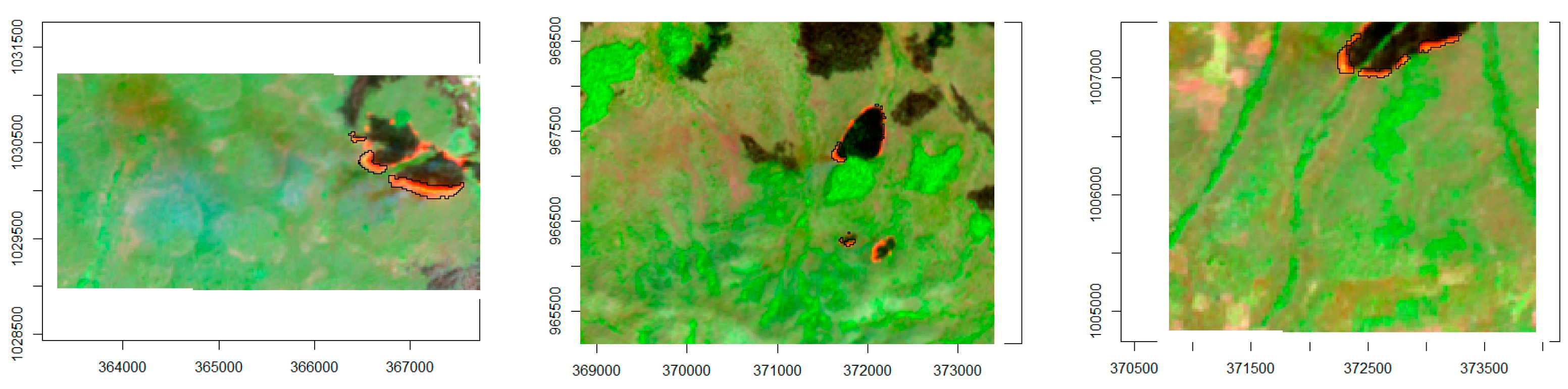
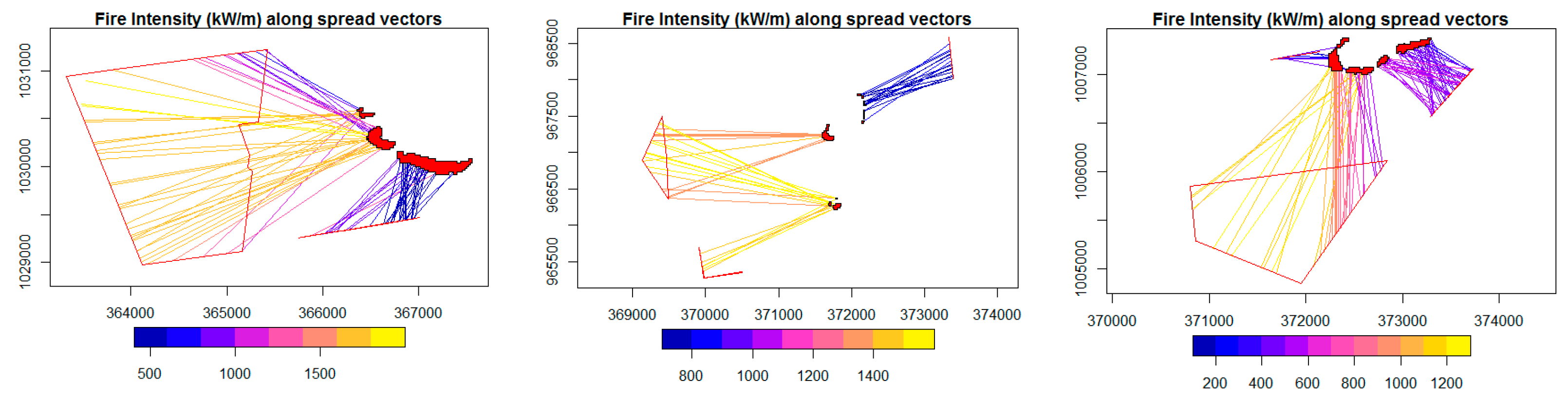
Figure 1, Figure 2, Figure 3, Figure 4 and Figure 5 illustrate the retrieval of ROS, FC and FI for three fire clusters that burned in the study area on November 20 and 25, 2020. Figure 1 shows the S-2 image subsets which were used to retrieve the S-2 fire fronts. Figure 2 illustrates the spread vectors which were constructed from the normals on the smoothed S-2 fire front edges, which were extended until the outer edge of the hull around the VIIRS fire detections from the NOAA 2 or S-NPP satellites. Depending on the frontal geometry, these hypothetical spread vectors can cross each other, which sometimes leads to unrealistic spread paths.
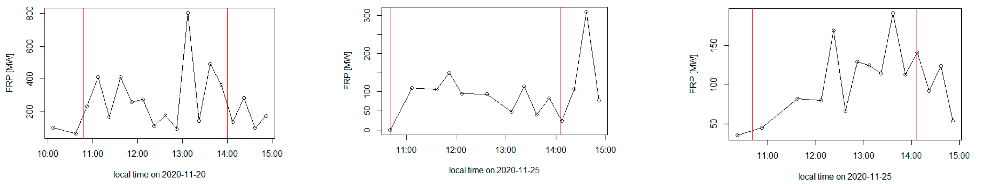
Figure 3 shows the summed FRP from Meteosat SEVIRI. This summation is based on a selection process of Meteosat active fire detections based on their proximity to any of the VIIRS and S-2 fire detections that are joined to each other through potential spread vectors. These envelopes are therefore in many cases larger than the footprints of the fire clusters in Figure 2 and Figure 5. This is due to the coarse spatial resolution which makes it impossible to resolve the FRP attributed to a specific fire cluster in more spatial detail. The relation to FC per unit area is illustrated in Figure 4, which shows the envelopes based on the S-2 and VIIRS fire detections which circumscribe the area that has potentially been burned between the S-2 and VIIRS overpasses. An unknown, though probably not very large, error is introduced here as fires may have ignited after the S-2 overpass and went out before the VIIRS overpass and therefore leave no traces in the burned area envelopes but do contribute to the FRP detected by Meteosat, which would lead to an overestimation of FC and consequently FI. FC per unit area is then derived from the burned area that was mapped by using S-2 data obtained after the S-2 overpass used for ROS analysis. Accuracy of the burned area product hence also influences FC estimates, as commission errors contribute to underestimating FC while omission errors contribute to overestimating FC. Artefacts can be seen for instance in the left panel of Figure 4, where the area in front of the S-2 fire fronts was not mapped as having been burned after the S-2 overpass.
3.2. Characteristics of the Observed Fire Clusters
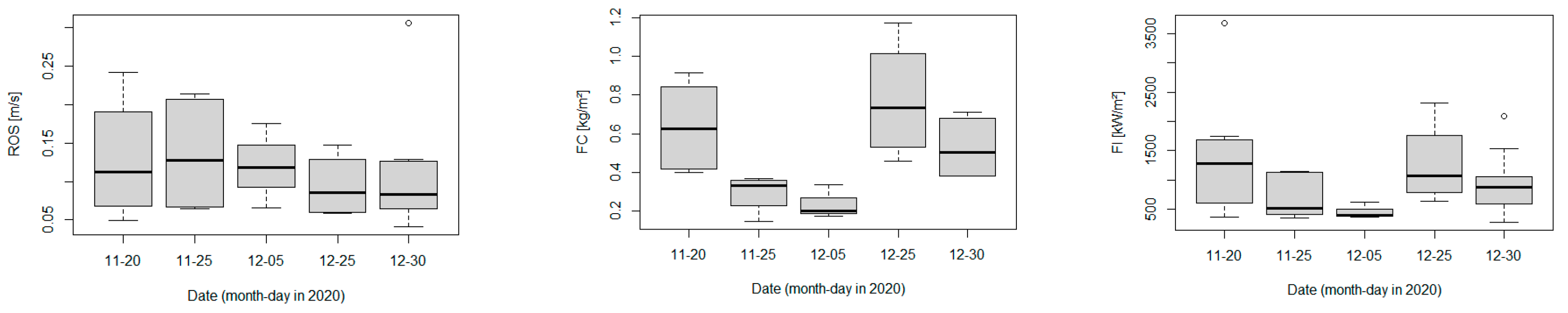
The analyzed fire clusters had a Meteosat-derived fuel consumption estimate ranging from 0.14 to 1.17 kg/m² with a mean of 0.49 kg/m² (sd: 0.27 kg/m²). Figure 6 shows boxplots of FC for the different dates analyzed. Late November and early December had lower fuel consumption than late December, which is consistent with the assumption that combustion completeness increases as fuel dries out with the progressing fire season. The ROS and FI estimates are presented as boxplots of summary statistics derived from the single spread vectors connecting the S-2 and VIIRS fronts analyzed. These measures were the mean of all connectors associated with one cluster, the means of the 0.75 quantile of the connectors within each analyzed fire cluster, and the mean of the 0.9 quantile of connectors. The mean of cluster means was 0.07 m/s, minimum cluster mean was 0.02 m/s, and maximum cluster mean was 0.21 m/s. These values include head, flanking and back fires. To obtain a better estimate for ROS attained by head fires, i.e., fires burning with the wind, the 0.75 and 0.9 quantiles of spread vectors for each fire cluster were analyzed. Mean of the 0.75 quantile over all days and clusters was 0.09 m/s (max: 0.29 m/s, min: 0.028 m/s), and mean of the 0.9 quantile was 0.11 m/s (min: 0.04 m/s, max: 0.3 m/s). No strong differences could be observed between the days analyzed. Boxplots for the 90% percentile are given in Figure 6. Mean of the mean fire intensities over all clusters was 608 kW/m (sd: 350 kW/m, min: 166 kW/m, max: 1510 kW/m). The mean of the 90% percentile of FI was 928 kW/m (min: 286 kW/m, max: 2316 kW/m, see Figure 6). Fire intensities were influenced by the fuel consumption estimates and were slightly higher in the late December observations (December 25 and 30) and lower in the late November and early December observations with the exception of November 20 that had a similar median FI as the late December observations, but a lower 0.75 quantile.
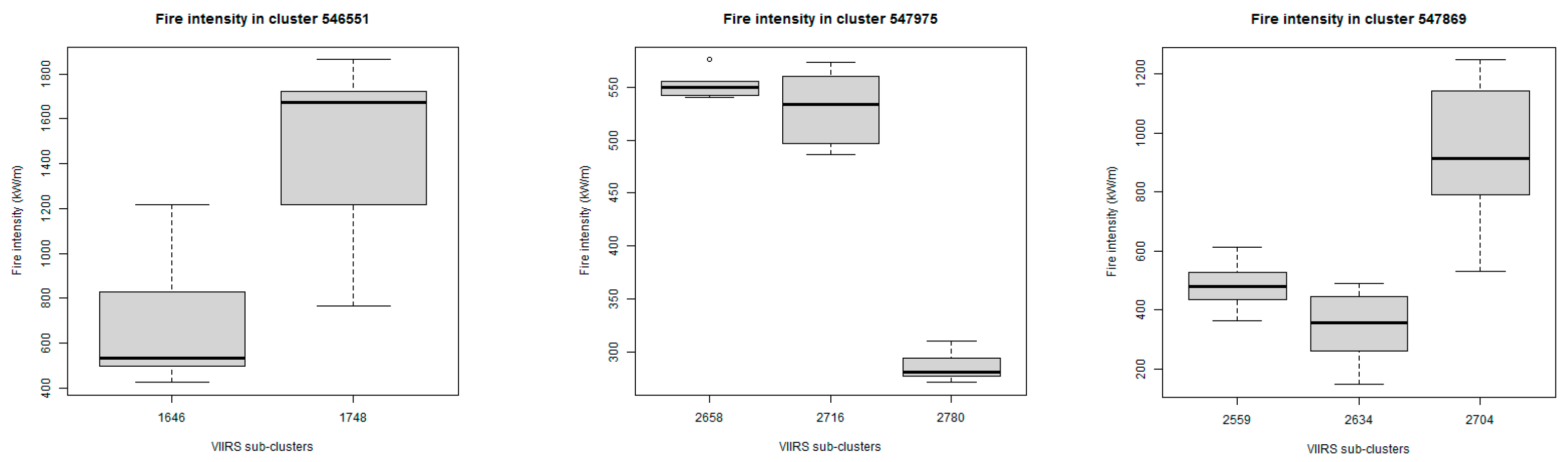
For some fires, it was possible to associate the head and flanking fires with VIIRS fire clusters, and in rare cases, head and back fires’ spread could be observed and associated with different VIIRS fire clusters. In Figure 7, boxplots of the fire intensity of the spread vectors of the clusters of Figure 2 and Figure 4 show that the flanking fires have substantially lower intensities (due to their lower spread rates) than the head fires. Equally, the back fire has a significantly lower intensity than the assumed head fires.
4. Discussion
We have developed and tested a method to directly estimate rate of spread and Byram’s fire or fireline intensity from satellite remote sensing observations using high (20 m), medium (375 m) and coarse resolution (~3 km) active fire data. Our methods differ from previous studies on spaceborne fire intensity [41,42,43] in that these works provided “radiative” fireline intensity, which is usually an order of magnitude lower than fireline intensity estimated in the field, while our approach tries to directly derive the main parameters of Byram’s classical equation from remote sensing data and hence yields fire intensity in similar numbers as those observed in the field. It is possible to independently validate the single input parameters to establish an error budget, e.g. through airborne experiments. Furthermore, rate of spread and fuel consumption, which are first-order measures of fire behavior [55], are estimated in addition to fire intensity.
Our fire intensity, rate of spread and fuel consumption estimates are similar to those obtained from field experiments in the region; they fall within the range found in CNP [54] and in the Lamto reserve which is located further South and has higher fuel loads and hence somewhat higher fire intensities than those observed in CNP [56]. The fire intensities and rate of spread observed in this study are in turn a bit higher than those measured in the field in a “working landscape” in southern Mali which is further north than our study site [57].
While these first results seem promising, application on a larger scale would still require a considerable research investment in developing a stable algorithm which would allow one to process a larger amount of data to, e.g., develop a fire intensity time series and fire climatology on the landscape scale. Such a data product could possibly complement existing products such as those defined for fire in the Essential Climate Variables concept (ECVs) [58], which are active fires, burned areas and FRP. Among the main issues that need to be addressed to produce an automated product in the future is the correct pairing of the Sentinel and VIIRS-derived fire fronts. Despite implementing the different tests described in the methods section, implausible connections between fronts have been selected, while at the same time, plausible connections had been removed by the original algorithm. Methods based on artificial intelligence such as pattern recognition could potentially help to establish a more robust method to perform the pairing. Regarding the establishment of the spread vectors themselves, the approach to simply extend the fire front normal until it hits a VIIRS front can possibly also be improved through other methods that find more likely pathways.
To establish an error budget, a prerequisite for a potential future product, errors in ROS and FC need to be constrained. ROS errors stem from locational error (influenced, i.a., by pixel size and point spread function of the sensors) in the position of the fire front and by the error in estimating the distance travelled by the fire front, whereas the error in the time difference (resulting from the sensor overpass times) can be neglected. Reference [59] showed for small-scale experiments that fire front rate of spread estimates are strongly influenced by measurement approach, and this also holds true for satellite-based observations. To evaluate errors stemming from the measurement approach, airborne experiments on experimental fires could be used to develop and test different approaches.
According to Byram [2,3], FC in fire intensity is the fuel consumed in the active flaming zone. However, in “traditional” fire experiments to derive fire intensity, FC in the active flaming zone cannot be separated from total FC, and this is in part used to explain the large differences between fire intensity and radiative fireline intensity [41]. On the other hand, FRP derived through the single-band MWIR method [15] is more sensitive to flaming combustion, and we do not assume that in predominantly flaming grass fires, a large error on FC can be attributed to the missing distinction between FRP generated in the flaming zone from total FRP. A substantially larger error stems from the conversion of FRP to FC, and as outlined in the introduction section of this paper, this is an area of active research, and there is a need for better constraining these relationships which are, e.g., used in the Copernicus Atmosphere Monitoring Service (CAMS) [27]. A further error is introduced by missing observations of the fire by the SEVIRI sensor, as well as by missing weaker radiating fires in general. We tried to reduce this error by excluding clusters with too many missing observations (see methods section). For the establishment of an error budget, resampling techniques, e.g., jacknife resampling [60], could be used to better constrain this error. To arrive at FC per unit area as needed in the fire intensity calculation, the division by the area that burned between the two observations of the fire front is needed. This quantity is influenced (a) by the accuracy of the assessment of burned area (in our test case derived from S-2 data), and (b) by the burned area envelope which is formed by the area enclosed by the connect S-2 and VIIRS fire fronts and their connecting spread vectors.
The approach demonstrated here can be carried to other sensors and other areas of the globe, ideally where geostationary satellites (currently, apart from Meteosat, the GOES [19] and Himawari [21] satellites) with a high temporal resolution and FRP retrievals provide the option to estimate fuel consumption over the Americas, parts of Asia and Australia as does Meteosat for Africa and parts of Europe and South America. For other parts of the world, our approach would still be feasible if coarser FC estimates can be performed from polar orbiting satellites or other sources. Within the next couple of years, the Meteosat Third Generation satellites will be equipped with a 1 km spatial resolution fire detection and characterization capability every ten minutes over Europe, Africa and parts of South America [61], which will substantially improve the ability to characterize fires and track single-fire events, e.g., for derivation of fire behavior parameters such as discussed here. Other upcoming instruments such as the planned Canadian WildFireSat mission [62] and the proposed DIEGO mission on the International Space Station [63] will provide additional opportunities to derive wildfire ROS at high spatial resolution at varying overpass times (DIEGO) and medium spatial resolution fire detection at a currently under-observed late afternoon overpass time (WildFireSat).
Author Contributions
Conceptualization, G.R.; methodology, G.R..; software, G.R. and D.L.; formal analysis, G.R., D.L. and J.T.; data curation, G.R., D.L. and J.T.; writing—original draft preparation, G.R.; writing—review and editing, G.R.; project administration, G.R.; funding acquisition, G.R. All authors have read and agreed to the published version of the manuscript.
Funding
This research was partially funded by the ZIM program of the German Ministry of Economy, grant number 16KN052420.
Data Availability Statement
Sentinel-2 data are available at https://scihub.copernicus.eu/, accessed on 1 July 2021, VIIRS data are available through FIRMS (https://earthdata.nasa.gov/firms, accessed on 1 July 2021) and Meteosat through EUMETSAT (https://landsaf.ipma.pt/en/, accessed on 1 July 2021).
Acknowledgments
The authors are grateful for the provision of free and open data, namely from NASA’s Fire Information for Resource Management System (FIRMS), part of NASA’s Earth Observing System Data and Information System (EOSDIS), the Copernicus program of the European Union, the NOAA polar orbiting satellite system programs and EUMETSAT, the operator of Meteosat.
Conflicts of Interest
The authors declare no conflict of interest.
References
- Govender, N.; Trollope, W.S.W.; Van Wilgen, B.W. The effect of fire season, fire frequency, rainfall and management on fire intensity in savanna vegetation in South Africa. J. Appl. Ecol. 2006, 43, 748–758. [Google Scholar] [CrossRef]
- Byram, G.M. Combustion of Forest Fuels. In Forest Fire: Control and Use; McGraw-Hill: New York, NY, USA, 1959; pp. 61–89. [Google Scholar]
- Alexander, M.E. Calculating and interpreting forest fire intensities. Can. J. Bot. 1982, 60, 349–357. [Google Scholar] [CrossRef]
- Wotton, B.M.; Flannigan, M.; Marshall, G.A. Potential climate change impacts on fire intensity and key wildfire suppression thresholds in Canada. Environ. Res. Lett. 2016, 12, 095003. [Google Scholar] [CrossRef]
- Williams, R.J.; Cook, G.D.; Gill, A.M.; Moore, P.H.R. Fire regime, fire intensity and tree survival in a tropical savanna in northern Australia. Austral. Ecol. 1999, 24, 50–59. [Google Scholar] [CrossRef]
- Miranda, A.C.; Miranda, H.; Dias, I.D.F.O.; Dias, B.F.D.S. Soil and air temperatures during prescribed cerated fires in Central Brazil. J. Trop. Ecol. 1993, 9, 313–320. [Google Scholar] [CrossRef]
- Lipsett-Moore, G.J.; Wolff, N.H.; Game, E.T. Emissions mitigation opportunities for savanna countries from early dry season fire management. Nat. Commun. 2018, 9, 2247. [Google Scholar] [CrossRef] [PubMed] [Green Version]
- Laris, P. On the problems and promises of savanna fire regime change. Nat. Commun. 2021, 12, 4891. [Google Scholar] [CrossRef] [PubMed]
- Johnston, J.M.; Wooster, M.J.; Paugam, R.; Wang, X.; Lynham, T.J.; Johnston, L.M. Direct estimation of Byram’s fire intensity from infrared remote sensing imagery. Int. J. Wildland Fire 2017, 26, 668. [Google Scholar] [CrossRef] [Green Version]
- Zhukov, B.; Lorenz, E.; Oertel, D.; Wooster, M.; Roberts, G. Spaceborne detection and characterization of fires during the bi-spectral infrared detection (BIRD) experimental small satellite mission (2001–2004). Remote Sens. Environ. 2006, 100, 29–51. [Google Scholar] [CrossRef]
- Kauffman, J.Y.; Justice, C.O.; Flynn, L.P.; Kendall, J.D.; Prins, E.M.; Giglio, L.; Ward, D.E.; Menzel, W.P.; Setzer, A.W. Potential global fire monitoring from EOS-MODIS. J. Geophys. Res. 1998, 103, 32215–32238. [Google Scholar] [CrossRef]
- Justice, C.; Giglio, L.; Korontzi, S.; Owens, J.; Morisette, J.T.; Roy, D.; Descloitres, J.; Alleaume, S.; Petitcolin, F.; Kaufman, Y. The MODIS fire products. Remote Sens. Environ. 2002, 83, 244–262. [Google Scholar] [CrossRef]
- Wooster, M.J.; Zhukov, B.; Oertel, D. Fire radiative energy for quantitative study of biomass burning: Derivation from the BIRD experimental satellite and comparison to MODIS fire products. Remote Sens. Environ. 2003, 86, 83–107. [Google Scholar] [CrossRef]
- Dozier, J. A method for satellite identification of surface temperature fields of subpixel resolution. Remote Sens. Environ. 1981, 11, 221–229. [Google Scholar] [CrossRef]
- Matson, M.; Dozier, J. Identification of subresolution high temperature sources using a thermal IR sensor. Photogramm. Eng. Remote Sens. 1981, 47, 1311–1318. [Google Scholar]
- Wooster, M.J.; Roberts, G.; Perry, G.; Kaufman, Y.J. Retrieval of biomass combustion rates and totals from fire radiative power observations: FRP derivation and calibration relationships between biomass consumption and fire radiative energy release. J. Geophys. Res. Space Phys. 2005, 110. [Google Scholar] [CrossRef]
- Schroeder, W.; Csiszar, I.; Giglio, L.; Schmidt, C.C. On the use of fire radiative power, area, and temperature estimates to characterize biomass burning via moderate to coarse spatial resolution remote sensing data in the Brazilian Amazon. J. Geophys. Res. Space Phys. 2010, 115. [Google Scholar] [CrossRef] [Green Version]
- Roberts, G.J.; Wooster, M.J. Fire Detection and Fire Characterization Over Africa Using Meteosat SEVIRI. IEEE Trans. Geosci. Remote Sens. 2008, 46, 1200–1218. [Google Scholar] [CrossRef] [Green Version]
- Xu, W.; Wooster, M.J.; He, J.; Zhang, T. Improvements in high-temporal resolution active fire detection and FRP retrieval over the Americas using GOES-16 ABI with the geostationary Fire Thermal Anomaly (FTA) algorithm. Sci. Remote Sens. 2021, 3, 100016. [Google Scholar] [CrossRef]
- Xu, W.; Wooster, M.; Roberts, G.; Freeborn, P. New GOES imager algorithms for cloud and active fire detection and fire radiative power assessment across North, South and Central America. Remote Sens. Environ. 2010, 114, 1876–1895. [Google Scholar] [CrossRef]
- Xu, W.; Wooster, M.; Kaneko, T.; He, J.; Zhang, T.; Fisher, D. Major advances in geostationary fire radiative power (FRP) retrieval over Asia and Australia stemming from use of Himarawi-8 AHI. Remote Sens. Environ. 2017, 193, 138–149. [Google Scholar] [CrossRef] [Green Version]
- Schroeder, W. Visible Infrared Imaging Radiometer Suite (VIIRS) 375 m & 750 m Active Fire Detection Data Sets Based on NASA VIIRS Land Science Investigator Processing System (SIPS) Reprocessed Data—Version 1, Product User Guide, NASA. 2017. Available online: https://lpdaac.usgs.gov/documents/132/VNP14_User_Guide_v1.3.pdf (accessed on 27 September 2021).
- Li, F.; Zhang, X.; Kondragunta, S.; Csiszar, I. Comparison of Fire Radiative Power Estimates From VIIRS and MODIS Observations. J. Geophys. Res. Atmos. 2018, 123, 4545–4563. [Google Scholar] [CrossRef]
- Giglio, L.; Schroeder, W.; Justice, C.O. The collection 6 MODIS active fire detection algorithm and fire products. Remote Sens. Environ. 2016, 178, 31–41. [Google Scholar] [CrossRef] [Green Version]
- Wooster, M.; Xu, W.; Nightingale, T. Sentinel-3 SLSTR active fire detection and FRP product: Pre-launch algorithm development and performance evaluation using MODIS and ASTER datasets. Remote Sens. Environ. 2012, 120, 236–254. [Google Scholar] [CrossRef]
- Xu, W.; Wooster, M.J.; He, J.; Zhang, T. First study of Sentinel-3 SLSTR active fire detection and FRP retrieval: Night-time algorithm enhancements and global intercomparison to MODIS and VIIRS AF products. Remote Sens. Environ. 2020, 248, 111947. [Google Scholar] [CrossRef]
- Kaiser, J.W.; Heil, A.; Andreae, M.O.; Benedetti, A.; Chubarova, N.; Jones, L.; Morcrette, J.-J.; Razinger, M.; Schultz, M.G.; Suttie, M.; et al. Biomass burning emissions estimated with a global fire assimilation system based on observed fire radiative power. Biogeosciences 2012, 9, 527–554. [Google Scholar] [CrossRef] [Green Version]
- Andela, N.; van der Werf, G.; Kaiser, J.W.; Van Leeuwen, T.T.; Wooster, M.; Lehmann, C. Biomass burning fuel consumption dynamics in the tropics and subtropics assessed from satellite. Biogeosciences 2016, 13, 3717–3734. [Google Scholar] [CrossRef] [Green Version]
- Roberts, G.; Wooster, M.J.; Xu, W.; He, J. Fire Activity and Fuel Consumption Dynamics in Sub-Saharan Africa. Remote Sens. 2018, 10, 1591. [Google Scholar] [CrossRef] [Green Version]
- Boschetti, L.; Roy, D.P. Strategies for the fusion of satellite fire radiative power with burned area data for fire radiative energy derivation. J. Geophys. Res. Space Phys. 2009, 114. [Google Scholar] [CrossRef] [Green Version]
- Schroeder, W.; Ellicott, E.; Ichoku, C.; Ellison, L.; Dickinson, M.; Ottmar, R.D.; Clements, C.; Hall, D.; Ambrosia, V.; Kremens, R. Integrated active fire retrievals and biomass burning emissions using complementary near-coincident ground, airborne and spaceborne sensor data. Remote Sens. Environ. 2014, 140, 719–730. [Google Scholar] [CrossRef] [Green Version]
- Hudak, A.T.; Dickinson, M.B.; Bright, B.C.; Kremens, R.L.; Loudermilk, E.L.; O’Brien, J.J.; Hornsby, B.S.; Ottmar, R.D. Measurements relating fire radiative energy density and surface fuel consumption—RxCADRE 2011 and 2012. Int. J. Wildland Fire 2016, 25, 25–37. [Google Scholar] [CrossRef] [Green Version]
- Schroeder, W.; Oliva, P.; Giglio, L.; Csiszar, I.A. The New VIIRS 375 m active fire detection data product: Algorithm description and initial assessment. Remote Sens. Environ. 2014, 143, 85–96. [Google Scholar] [CrossRef]
- Lorenz, E.; Mitchell, S.; Säuberlich, T.; Paproth, C.; Halle, W.; Frauenberger, O. Remote Sensing of High Temperature Events by the FireBird Mission. ISPRS—Int. Arch. Photogramm. Remote Sens. Spat. Inf. Sci. 2015, XL-7/W3, 461–467. [Google Scholar] [CrossRef] [Green Version]
- Caseiro, A.; Rücker, G.; Tiemann, J.; Leimbach, D.; Lorenz, E.; Frauenberger, O.; Kaiser, J.W. Persistent Hot Spot Detection and Characterisation Using SLSTR. Remote Sens. 2018, 10, 1118. [Google Scholar] [CrossRef] [Green Version]
- Fisher, D.; Wooster, M.J. Shortwave IR Adaption of the Mid-Infrared Radiance Method of Fire Radiative Power (FRP) Retrieval for Assessing Industrial Gas Flaring Output. Remote Sens. 2018, 10, 305. [Google Scholar] [CrossRef] [Green Version]
- Elvidge, C.D.; Zhizhin, M.; Hsu, F.-C.; Baugh, K.E. VIIRS Nightfire: Satellite Pyrometry at Night. Remote Sens. 2013, 5, 4423–4449. [Google Scholar] [CrossRef] [Green Version]
- Schroeder, W.; Oliva, P.; Giglio, L.; Quayle, B.; Lorenz, E.; Morelli, F. Active fire detection using Landsat-8/OLI data. Remote Sens. Environ. 2016, 185, 210–220. [Google Scholar] [CrossRef] [Green Version]
- Kumar, S.S.; Roy, D.P. Global operational land imager Landsat-8 reflectance-based active fire detection algorithm. Int. J. Digit. Earth 2018, 11, 154–178. [Google Scholar] [CrossRef] [Green Version]
- Sofan, P.; Bruce, D.; Jones, E.; Khomarudin, M.; Roswintiarti, O. Applying the Tropical Peatland Combustion Algorithm to Landsat-8 Operational Land Imager (OLI) and Sentinel-2 Multi Spectral Instrument (MSI) Imagery. Remote Sens. 2020, 12, 3958. [Google Scholar] [CrossRef]
- Wooster, M.J.; Perry, G.L.W.; Zhukov, B.; Oertel, D. Estimation of Energy. In Spatial Modelling of the Terrestrial Environment; Kelly, R., Drake, N., Barr, S., Eds.; John Wiley & Sons: London, UK, 2004. [Google Scholar]
- Wooster, M.J.; Zhang, Y. Boreal forest fires burn less intensely in Russia than in North America. Geophys. Res. Lett. 2004, 31, L20505. [Google Scholar] [CrossRef] [Green Version]
- Smith, A.M.S.; Wooster, M.J. Remote classification of head and backfire types from MODIS fire radiative power and smoke plume observations. Int. J. Wildland Fire 2005, 14, 249. [Google Scholar] [CrossRef] [Green Version]
- Paugam, R.; Wooster, M.; Roberts, G. Use of Handheld Thermal Imager Data for Airborne Mapping of Fire Radiative Power and Energy and Flame Front Rate of Spread. IEEE Trans. Geosci. Remote Sens. 2012, 51, 3385–3399. [Google Scholar] [CrossRef]
- Ononye, A.E.; Vodacek, A.; Saber, E. Automated extraction of fire line parameters from multispectral infrared images. Remote Sens. Environ. 2007, 108, 179–188. [Google Scholar] [CrossRef] [Green Version]
- Hu, X.; Ban, Y.; Nascetti, A. Sentinel-2 MSI data for active fire detection in major fire-prone biomes: A multi-criteria approach. Int. J. Appl. Earth Obs. Geoinf. 2021, 101, 102347. [Google Scholar] [CrossRef]
- Ester, M.; Kriegel, H.P.; Sander, J.; Xu, X. A density-based algorithm for discovering clusters in large spatial databases with noise. In Proceedings of the Second International Conference on Knowledge Discovery and Data Mining (KDD’96), Portland, Oregon, 2–4 August 2016; AAAI Press: Palo Alto, CA, USA, 1996; pp. 226–231. [Google Scholar]
- García, M.J.L.; Caselles, V. Mapping burns and natural reforestation using thematic Mapper data. Geocarto Int. 1991, 6, 31–37. [Google Scholar] [CrossRef]
- Trigg, S.; Flasse, S. An evaluation of different bi-spectral spaces for discriminating burned shrub-savannah. Int. J. Remote Sens. 2001, 22, 2641–2647. [Google Scholar] [CrossRef]
- Zhu, Z.; Wang, S.; Woodcock, C.E. Improvement and expansion of the Fmask algorithm: Cloud, cloud shadow, and snow detection for Landsats 4–7, 8, and Sentinel 2 images. Remote Sens. Environ. 2015, 159, 269–277. [Google Scholar] [CrossRef]
- Goetze, D.; Hörsch, B.; Porembski, S. Dynamics of forest-savanna mosaics in north-eastern Ivory Coast from 1954 to 2002. J. Biogeogr. 2006, 33, 653–664. [Google Scholar] [CrossRef]
- Soro, T.D.; Soro, T.D.; Koné, M.; N’Dri, A.B.; N’Datchoh, E.T. Identified main fire hotspots and seasons in Cote d’lvoire (West Africa) using MODIS fire data. S. Afr. J. Sci. 2021, 117, 1–13. [Google Scholar]
- Hennenberg, K.J.; Fischer, F.; Kouadio, K.; Goetze, D.; Orthmann, B.; Linsenmair, K.E.; Jeltsch, F.; Porembski, S. Phytomass and fire occurrence along forest–savanna transects in the Comoé National Park, Ivory Coast. J. Trop. Ecol. 2006, 22, 303–311. [Google Scholar] [CrossRef]
- Ruecker, G. Suivi des Feux au Parc National de la Comoé et dans Ses Zones Périphériques (Warigué et Mt. Tingui) par Télédétection Pendant la Saison Sèche 2018/2019; Rapport de Projet; GIZ-Profiab II: Munich, Germany, 2019. [Google Scholar]
- Kremens, R.L.; Smith, A.; Dickinson, M. Fire Metrology: Current and Future Directions in Physics-Based Measurements. Fire Ecol. 2010, 6, 13–35. [Google Scholar] [CrossRef]
- N’Dri, A.B.; Soro, T.D.; Gignoux, J.; Dosso, K.; Koné, M.; N’Dri, J.K.; Koné, N.A.; Barot, S. Season affects fire behavior in annually burned humid savanna of West Africa. Fire Ecol. 2018, 14, 5. [Google Scholar] [CrossRef]
- Laris, P.; Jacobs, R.; Koné, M.; Dembélé, F.; Rodrigue, C.M. Determinants of fire intensity in working landscapes of an African savanna. Fire Ecol. 2020, 16, 27. [Google Scholar] [CrossRef]
- Bojinski, S.; Verstraete, M.; Peterson, T.C.; Richter, C.; Simmons, A.; Zemp, M. The Concept of Essential Climate Variables in Support of Climate Research, Applications, and Policy. Bull. Am. Meteorol. Soc. 2014, 95, 1431–1443. [Google Scholar] [CrossRef]
- Johnston, J.M.; Wheatley, M.J.; Wooster, M.J.; Paugam, R.; Davies, G.M.; DeBoer, K.A. Flame-Front Rate of Spread Estimates for Moderate Scale Experimental Fires Are Strongly Influenced by Measurement Approach. Fire 2018, 1, 16. [Google Scholar] [CrossRef] [Green Version]
- Friedl, H.; Stampfer, E. Jackknife resampling. Encycl. Environ. 2002, 2, 1089–1098. [Google Scholar]
- Holmlund, K.; Grandell, J.; Schmetz, J.; Stuhlmann, R.; Bojkov, B.; Munro, R.; Lekouara, M.; Coppens, D.; Viticchie, B.; August, T.; et al. Meteosat Third Generation (MTG): Continuation and Innovation of Observations from Geostationary Orbit. Bull. Am. Meteorol. Soc. 2021, 102, E990–E1015. [Google Scholar] [CrossRef]
- Johnston, J.M.; Jackson, N.; Mcfayden, C.; Phong, L.N.; Lawrence, B.; Davignon, D.; Wooster, M.J.; Van Mierlo, H.; Thompson, D.K.; Cantin, A.S.; et al. Development of the User Requirements for the Canadian WildFireSat Satellite Mission. Sensors 2020, 20, 5081. [Google Scholar] [CrossRef]
- Schultz, J.A.; Hartmann, M.; Heinemann, S.; Janke, J.; Jürgens, C.; Oertel, D.; Rücker, G.; Thonfeld, F.; Rienow, A. DIEGO: A Multispectral Thermal Mission for Earth Observation on the International Space Station. Eur. J. Remote Sens. 2019, 53, 28–38. [Google Scholar] [CrossRef] [Green Version]
Figure 1.
False color S-2 images of 20 (left) and 25 November 2020 (center and right panel) which were used as starting points for estimating ROS for the examples presented in Figure 2 ff. The detected S-2 fire fronts which were used for the ROS determination are marked with black outlines. Coordinates on the axes for all maps are UTM coordinates (in m) for UTM zone 30 N.

Figure 2.
Rate-of-spread vectors color coded by ROS (m/min) for the S-2 observations in Figure 1. Red filled polygons correspond to S-2 fire detections, red outlined polygons correspond to the concave hull shapes constructed from the VIIRS fire detection pixel center points. The images may have VIIRS fire detection envelopes from different overpasses (associated with NOAA 20 and S-NPP satellites) and hence spread vectors of similar length may have different associated ROS measures. The numbers on or near the VIIRS fire detection envelopes correspond to the associated boxplots in Figure 7.

Figure 3.
Summed Meteosat SEVIRI FRP over the fire front clusters depicted in Figure 1 and Figure 2. Red vertical lines indicate the times of the S-2 (left line) and VIIRS (right line) overpasses which were used for the temporal integration and creation of the burned area envelopes.

Figure 4.
Burned area envelopes over the fire front clusters depicted in Figure 1, Figure 2 and Figure 3. Gray areas have been mapped as burned using S-2, red polygons correspond to S-2 fire detections and red outlines to VIIRS fire detection envelopes. Red dots are the center coordinates of the VIIRS fire detection pixels.

Figure 5.
Color coded fire intensities (kW/m) derived for the fire fronts of Figure 1 and Figure 2 (for further details refer to Figure 2).

Figure 6.
Boxplots of ROS (left), FC (middle) and FI (right) of the analyzed fire clusters. ROS and FI values represent the means of the 90% quantiles of the fire spread vectors over the different fire clusters. Number of observations are: 11-20:8, 11-25:6, 12-05:3, 12-25:4, 12-30:9.
Figure 6.
Boxplots of ROS (left), FC (middle) and FI (right) of the analyzed fire clusters. ROS and FI values represent the means of the 90% quantiles of the fire spread vectors over the different fire clusters. Number of observations are: 11-20:8, 11-25:6, 12-05:3, 12-25:4, 12-30:9.

Figure 7.
Boxplots of FI for VIIRS fire clusters that could visually be associated with head fires and flanking fires (left and right panel) and head and backing fires (middle panel). The fire clusters correspond to those depicted in Figure 2 ff (in the same left-to-right order). The numbers of the VIIRS subclusters on the x-axis correspond to the numbers on or near these clusters in Figure 2.


Table 1.
Overview of satellite sensors used in this study.
| Platform | Sensor | Spatial Resolution 1 | Observation Times | Use in the Study |
|---|---|---|---|---|
| Sentinel 2A and 2B | MSI | 20 m | ~10:40, every five days | ROS, 1st obs.; burned area |
| S-NPP and NOAA 20 | VIIRS | 375 m | ~13:30–15:00 and 01:30–3:00, daily | ROS, 2nd obs. |
| Meteosat | SEVIRI | 3 km | Every 15 min | Fuel consumption |
1 Spatial resolution varies depending on the viewing angle for VIIRS and Meteosat.
Publisher’s Note: MDPI stays neutral with regard to jurisdictional claims in published maps and institutional affiliations. |
© 2021 by the authors. Licensee MDPI, Basel, Switzerland. This article is an open access article distributed under the terms and conditions of the Creative Commons Attribution (CC BY) license (https://creativecommons.org/licenses/by/4.0/).
Share and Cite
MDPI and ACS Style
Ruecker, G.; Leimbach, D.; Tiemann, J. Estimation of Byram’s Fire Intensity and Rate of Spread from Spaceborne Remote Sensing Data in a Savanna Landscape. Fire 2021, 4, 65. https://0-doi-org.brum.beds.ac.uk/10.3390/fire4040065
AMA Style
Ruecker G, Leimbach D, Tiemann J. Estimation of Byram’s Fire Intensity and Rate of Spread from Spaceborne Remote Sensing Data in a Savanna Landscape. Fire. 2021; 4(4):65. https://0-doi-org.brum.beds.ac.uk/10.3390/fire4040065
Chicago/Turabian StyleRuecker, Gernot, David Leimbach, and Joachim Tiemann. 2021. "Estimation of Byram’s Fire Intensity and Rate of Spread from Spaceborne Remote Sensing Data in a Savanna Landscape" Fire 4, no. 4: 65. https://0-doi-org.brum.beds.ac.uk/10.3390/fire4040065