Evaluating the Persistence of Post-Wildfire Ash: A Multi-Platform Spatiotemporal Analysis

Abstract

As wildland fires amplify in size in many regions in the western USA, land and water managers are increasingly concerned about the deleterious effects on drinking water supplies. Consequences of severe wildfires include disturbed soils and areas of thick ash cover, which raises the concern of the risk of water contamination via ash. The persistence of ash cover and depth were monitored for up to 90 days post-fire at nearly 100 plots distributed between two wildfires in Idaho and Washington, USA. Our goal was to determine the most ‘cost’ effective, operational method of mapping post-wildfire ash cover in terms of financial, data volume, time, and processing costs. Field measurements were coupled with multi-platform satellite and aerial imagery collected during the same time span. The image types spanned the spatial resolution of 30 m to sub-meter (Landsat-8, Sentinel-2, WorldView-2, and a drone), while the spectral resolution spanned visible through SWIR (short-wave infrared) bands, and they were all collected at various time scales. We that found several common vegetation and post-fire spectral indices were correlated with ash cover (r = 0.6–0.85); however, the blue normalized difference vegetation index (BNDVI) with monthly Sentinel-2 imagery was especially well-suited for monitoring the change in ash cover during its ephemeral period. A map of the ash cover can be used to estimate the ash load, which can then be used as an input into a hydrologic model predicting ash transport and fate, helping to ultimately improve our ability to predict impacts on downstream water resources.

1. Introduction

Consistent and accurate mapping of wildland fires is a critical function for active fire management as well as for post-fire mitigation and monitoring regimes. Wildfires play important ecological and hydrological roles in forests and have become larger and more frequent in the western USA in recent years [1]. This trend is expected to endure as summers continue to be longer and drier, and the effects of fire suppression and wildland–urban interface (WUI) encroachment persist in many regions [2,3,4]. Severe wildfires considerably alter the ground surface composition in spatially complex ways [5] due to the variable combustion of organic materials (vegetation, downed wood, litter, and duff), which can result in secondary effects such as increased surface runoff and erosion [6,7,8]. Wildfires combust organic matter into ash or char ranging from gray or white non-aggregate or airy materials to black, charred, and semi-recognizable organic matter. The presence of ash cover indicates combustion at high temperatures and long fire residence time [9,10,11]. Following Brewer et al. [12], for our purposes, “ash” is functionally defined as partially or fully combusted organic material that is available for transport via wind or water.

The presence of ash can alter the hydrologic response through the formation of surface seals in post-fire systems by creating a low conductive ash layer through soil pore sealing [13,14,15]; through an ash crust [13,16]; or through ash chemistry [17,18]. The increased potential for hydrologic activity can persist for several years depending on the severity of the wildfire disturbance [19]. Post-fire runoff and erosion can indicate soil (sediment) transportation but may also include ash transport and the potential nutrient and chemical pollutants attributed to ash [20,21,22]. Water quality degradation is likely if elevated runoff, soil erosion, or ash transport occurs after the wildfire [18,22,23]. Scientists have raised awareness regarding wildfire ash impacts on drinking water supplies particularly in areas that experience severe wildfires [24,25].

Ash is highly transportable via both wind and water; therefore, its attenuation rate after a fire is a function of the cumulative erosivity of wind and rainfall events [26]. Over time and after intense precipitation or wind events, ash changes color, density, and is ultimately transported from the site by water, wind, or is fully incorporated into the soil. Little is known about the persistence of ash on site in the post-wildfire environment, neither in terms of its duration, depth, nor fate [16,27]. To predict or model the effects of ash on post-fire runoff and erosion, it is first necessary to quantify the extent (cover) and load (e.g., mass per area, t·ha⁻¹) of ash while it is still on site [18]. Ash may change color over time as it is wetted or incorporated into the soil. The cover, load, and spatial distribution of ash must be considered when evaluating post-fire runoff and erosion potential [15,19,26]. Therefore, timely operational mapping of ash, similar to rapid burn severity mapping [28], would provide water managers with information to help minimize impacts on drinking water [5,22]. Accuracy and efficiency of information delivery are needed in real-time but also in the months and years following large wildfires.

Post-fire ash transport models are being developed [24] and a principle motivation of this study is working towards a methodology for quantifying ash after wildfires for use in these models [29]. To predict the transport and fate of ash (or any pollutant), a model needs a spatially explicit estimate of the amount or load available for transport. Ash is ephemeral and variable [30,31], and the relationship between burn severity and ash cover, depth, and load is not always predictable [27]. Optical remote sensing has shown promise for mapping ash cover [9,32,33] and even load [34], although these methods have not been widely implemented. A spatially explicit map of ash load is used as an input into a hydrologic model, such as the Water Erosion Prediction Project cloud-Wildfire Ash Transport and Risk (WEPPcloud-WATAR) model, and together with topographic, soil, and climate data, it is used to predict the delivery of ash and the associated contaminants to water bodies [24]. These modelling exercises are practical and applied rather than theoretical and are widely used by land managers around the world to plan and mitigate post-wildfire hydrologic disasters. Thus, reliable ash cover and load estimates are needed for model inputs, which greatly affect model predictive capabilities. Additionally, developing an operational method to map ash that is repeatable, time-sensitive, and can be seamlessly incorporated into watershed models is desirable.

Landscape-scale wildfire mapping is largely achieved with remote sensing across various platforms at multiple spatial, spectral, and temporal scales. Methodological approaches are widely implemented with Earth observation (EO) satellite data. Satellite imagery is used to create burn severity maps which highlight the change between pre and post-fire vegetation and soil conditions [28,31,35,36,37]. More recently, drones or unmanned aircraft systems (UASs) have been utilized to map fire perimeters and collect images of the burned area [38]. UASs are becoming a more common component of wildfire responses by providing emergency personnel with rapid situational awareness as well as creating maps of the burned areas [39]. Unlike a manned aircraft or a satellite under emergency fire situations, a UAS deployment can be more flexible and safer in terms of timing, location, and environmental conditions [40].

There are timing, data quality, and data quantity tradeoffs and considerations when choosing an imaging platform [41]. A UAS can collect ultra-high spatial resolution and true-color images on demand that are readily interpretable by non-experts [42], but often these have fewer spectral bands, limiting their use for higher-level image analysis. High spatial resolution commercial satellite imagery such as WorldView-2 (MAXAR, Longmont, CO) has 2 m pixels but must be tasked (ordered) and can be costly. An EO satellite such as Sentinel-2 which has 10 m pixels and a 5-day Earth-repeat orbit delivers visible through short-wave infrared (SWIR) bands, which are commonly used for post-fire mapping.

The goal of this study was to develop an operational and deliverable methodology for mapping post-fire ash, particularly one that can be used on different platforms and at multiple spatial scales depending on the data available and the ‘cost-benefit’ of the management need. We summarize our findings in a decision table, providing guidance on imagery, timing, and cost for post-fire mapping. To reach our study goal, we addressed the following specific objectives: (1) evaluate post-wildfire ash cover and depth in situ and monitor the change during its transitional period up to 90 days post-fire; and (2) compare moderate and high-resolution remotely sensed imagery for mapping ash cover and persistence over a time series. Meeting these objectives would help overcome current barriers to developing an operational mapping technique that can later be directly incorporated into hydrologic modelling.

2. Materials and Methods

2.1. Site Descriptions

The Mesa Fire started on 26 July 2018 in the Payette National Forest in Idaho and burned 14,100 ha over 4 weeks. Extreme fire behavior (https://www.fs.usda.gov/Internet/FSE_DOCUMENTS/fseprd616768.pdf, accessed on 10 September 2021) occurred during the first several days, driven by near record-high temperatures and strong winds. Approximately 400 ha within the Payette National Forest boundary were classified as having high soil burn severity and field sites were located in low, moderate, and high soil burn severity areas as determined from the burn severity map (Figure 1).

The Mesa Fire burned in a range of vegetation types from grassland to sagebrush-steppe; however, our study area coincided with the area of the highest severity burn, which was primarily classified by LANDFIRE (https://landfire.gov/, accessed on 10 September 2021) as Northern Rocky Mountain Dry-Mesic Montane Mixed Conifer Forest. Weather data from the nearest SNOTEL (Snow Telemetry) station Squaw Flat (1900 m elevation) gave an average annual precipitation (period of record: 1981$–$2010) of 1126 mm and maximum and minimum temperatures of 34 and −24 °C (https://www.wcc.nrcs.usda.gov/wps/portal/wcc/home, accessed on 6 October 2021). We also collected rainfall data with an onsite tipping bucket rain gauge (Figure 2).

The Redford Canyon Fire burned 335 ha in July 2017 on the Colville Indian Reservation in Washington (Figure 1). We sampled this small fire as a pilot-scale study the year before the Mesa Fire. Burn severity was mixed but primarily classified as moderate; however, there was sufficient ash on the ground for our research objectives. The fire burned in a temperate dry forest with open stands of Douglas-fir (Pseudotsuga menziesii) mixed with ponderosa pine (Pinus ponderosa) [43]. Field data were collected shortly after the fire in 2017: on 25 July, 8 August, 30 August and 27 September. Ash depths were collected at 9 spatially distributed plots along each of the 4 transects, along with spectral libraries of several different ash conditions. Sentinel-2 images from 9 July, 27 July, 18 August and 27 September in the same year were used to calculate spectral indices to compare to the field conditions and to the patterns in the imagery from the Mesa Fire.

2.2. Field Site Characterization

Field visits were initiated as soon as it was deemed safe to enter the burned area by local fire management teams [44]. Our goal was to sample sites at least every 2 weeks in the first month, with visits extending to every 4 weeks before significant freezing or precipitation occurred. Post-fire ash is ephemeral but the timeline of persistence is relatively unknown. The Mesa Fire field visit dates alongside the corresponding image collection dates are provided (Figure 3). The vertical shading clusters field visits with the closest Sentinel-2 pass.

Six 200 m transects were located in the Mesa Fire in low, moderate, and high-burn severity areas as identified from the burn severity map, which was created from classified Sentinel-2 imagery (Figure 1). At each transect endpoint (0 m and 200 m), 4 radial plots were located 30 m away, giving each endpoint 5 plots (1 center, 4 radial), totaling 10 plots per transect. Similar protocols were used at the Redford Canyon pilot study, with 4 transects and 9 radial plots per transect. Considering that all plots were to be revisited several times over 3+ months, extreme care was taken to minimize disturbance and GPS locations were collected with a Trimble Geo-XT GPS unit (Trimble Inc., Sunnyvale, CA, USA) with sub-meter accuracy. The initial visit to each plot was marked with a pin flag and each subsequent visit was approximately 1 m uphill. All plots were sampled 3 times and the 2 high-severity transects (Mesa Fire only) were sampled 4 times (Figure 3).

At each plot for each field visit, 4 high-resolution photos (Figure 4) were taken of the 4 quadrants of the 1 m plot. Field photographs of each quadrat, totaling an area of 1 m², were later loaded into the Cover Monitoring Assistant [45], for which the area was overlain by a grid for analysis. Each location was interpreted and counted, totaling to 100 points per quadrat, to provide an estimate of the macroscopic ash and char cover per quadrat.

A 0.2 m metal frame was used to delineate a smaller random portion of the plot for 5 ash-depth measurements and a total ash collection. A surface soil composite sample was collected below the ash layer at the center plot of each transect end. Soil and ash samples were collected in sealed bags and taken to the lab for drying and weighing. Ash bulk density was calculated from the weight and volume of some of the ash samples.

By the end of the study period (90 days post-fire), all plots had received rain (Figure 2) and experienced freeze–thaw cycles. It was difficult at this point to discern dark, wet soil from dark, charred soil (Figure 4); thus, the field sampling was concluded.

2.3. Image Acquisition and Analysis

All Mesa Fire imagery was collected during the period of 8 July to 20 October 2018, which spanned from 21 days prior to the fire ignition to ~90 days after the fire (Figure 3). The only imagery that was used for the Redford Canyon Fire was Sentinel-2 imagery, which was collected over a post-fire period of 80 days.

Sentinel-2 and Landsat-8 images were selected from open access data archives for quality, limited cloud cover, and for timing relative to the field data collections. Sentinel-2 (S2) was launched by the European Space Agency (ESA). Revisit time was approximately 5 days and the spatial resolution was from 10 m to 20 m, spanning the visible through the SWIR region (

Table 1. Satellite information: central bands, bandwidth span, and pixel size (spatial resolution). NIR is near-infrared and SWIR is short-wave infrared.

	Landsat-8			Sentinel-2			WorldView-2
Band	Central Wavelength (nm)	Span (nm)	Pixel (m)	Central Wavelength (nm)	Span (nm)	Pixel (m)	Central Wavelength (nm)	Span (nm)	Pixel (m)
Blue	482 [B2]	435–451	30	492 [B2]	459–525	10	478 [B2]	450–510	1.8
Green	561 [B3]	452–512	30	560 [B3]	542–578	10	546 [B3]	510–580	1.8
Red	655 [B4]	636–673	30	665 [B4]	650–681	10	659 [B5]	630–690	1.8
NIR	865 [B5]	851–879	30	833 [B8a] 1	780–886	10	831 [B7]	770–895	1.8
SWIR1	1609 [B6]	1567–1651	30	1614 [B11]	1569–1660	20	-	-	-
SWIR2	2201 [B7]	2107–2294	30	2202 [B12]	2115–2290	20	-	-	-

¹ Band 8a is the narrower NIR band and has a closer spectral correspondence to the NIR band of Landsat-8.

). The Landsat-8 (L8) satellite is a collaboration between NASA (National Aeronautics and Space Administration) and the USGS (United States Geological Survey), and has a revisit frequency of 16 days and a 30 m spatial resolution over all bands. Both S2 and L8 data were freely available for download via open-access hubs. All S2 images were downloaded and pre-processed to the bottom of the atmosphere reflectance with Sen2Cor [46] using the sen2r package in R [47]. Landsat Level-2 surface reflectance science products were downloaded. We expected that both the higher revisit frequency and higher spatial resolution of S2 images would lend to improvements over Landsat; however, Landsat data has been the baseline post-fire imagery and provides a benchmark for post-fire remote sensing studies over many years, therefore we included it in our analysis.

A single WorldView-2 image of the entire burned area that had been previously tasked by another user was retrieved from the digital archive (https://discover.digitalglobe.com/, accessed on 8 September 2021). WorldView-2 (WV2) (MAXAR Technologies, Longmont, CO) imagery has a pixel size of 1.8 m across the visible and near infrared (NIR) bands (Table 1). One WV2 image of the entire burned area spanned 2 tiles, which were downloaded and already georeferenced. The residual geometric error was corrected by automatic orthorectification to a 10 m DEM (digital elevation model) reference image using rational polynomial coefficients (RPCs) provided by the vendor using a nearest neighbor method (in ESRI ArcMap 10.5.1). The resulting root mean square error (RMSE) of the position was below one pixel. A dark object subtraction was done to remove atmospheric scattering using band minimums (in ENVI 4.2, L3Harris Geospatial, Boulder, CO, USA) and to correct the data to surface reflectance.

Ancillary UAS imagery for this project was acquired in collaboration with the faculty and students at Northwest Nazarene University (NNU; Nampa, ID). Images were collected with a DJI (Da-Jiang Innovations) Phantom 4 drone with a 12-megapixel Red-Green-Blue (RGB) color camera [40]. The imagery acquired with the UAS was taken while flying at an altitude of 120 m above the ground level, giving the photos a spatial resolution of 6 cm per pixel. Due to time and data volume constraints, only the area over the study transects was imaged. Three separate images were acquired that intentionally coincided with the field sampling dates (Figure 3).

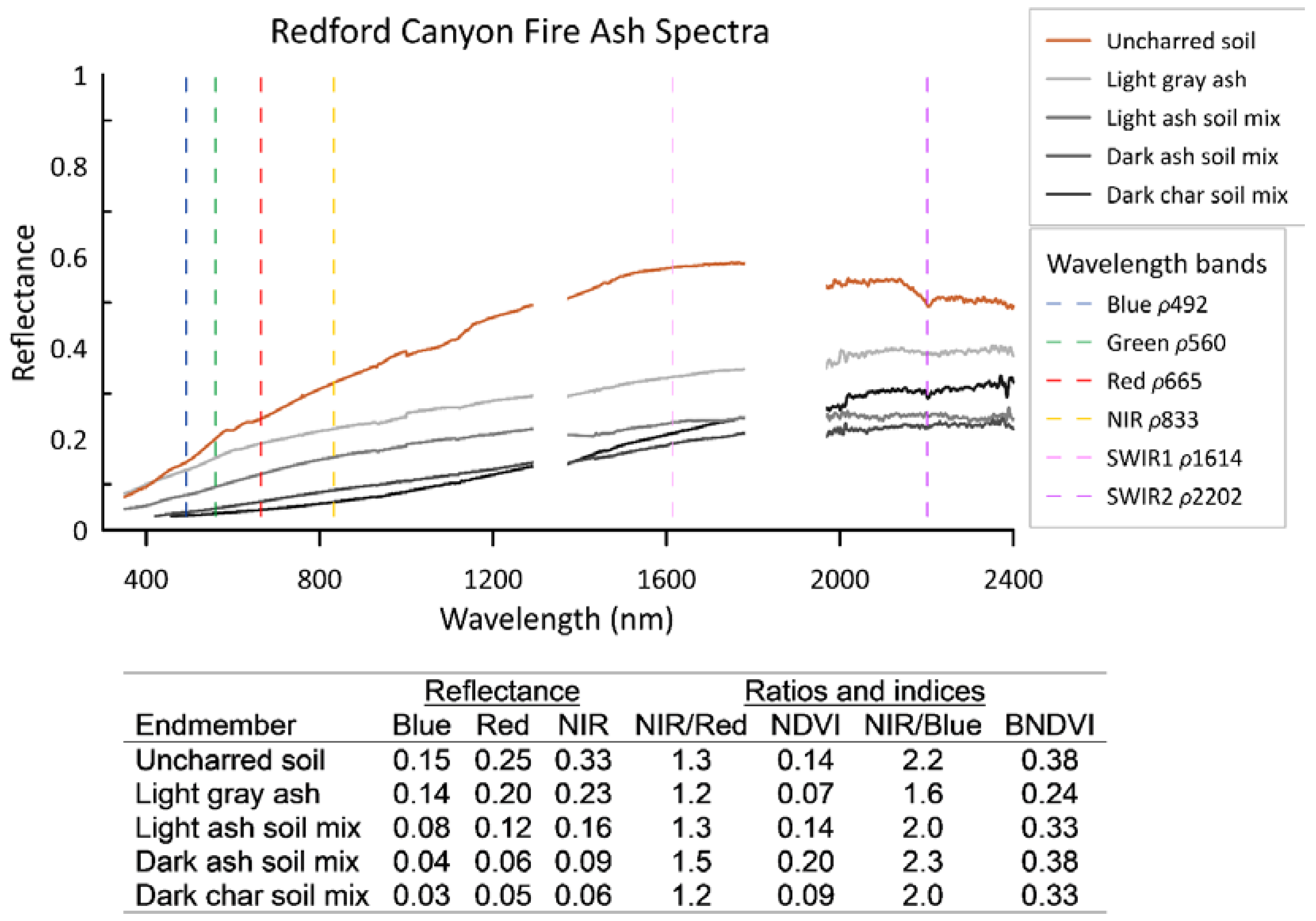
2.4. Endmember Spectra Collection

Endmember spectra of soil, ash, and char were collected after the Redford Canyon Fire on a cloud-free day within 2 h of solar noon using an ASD Pro-FR field spectroradiometer (Analytical Spectral Devices, Inc., Boulder, CO, USA). Spectra were collected with the bare-tip foreoptic (field of view 22°) pointed at the target material from a height of ~1 m. The ASD Pro-FR sampling interval was 1.4 nm over the 350 to 1050 nm wavelength range and 2 nm over the 1000 to 2500 nm range. These measurements were interpolated at every 1 nm wavelength and reported in 2151 contiguous channels. The field spectrometer was calibrated against a Spectralon (Labsphere, North Sutton, NH, USA) 100% reflective panel immediately before and at frequent intervals during field spectra collection to account for changing light and atmospheric conditions. Absolute reflectance was calculated at the time of data collection for all spectra by dividing the field reflectance by the bright target reflectance.

2.5. Spectral Indices

Prior to a wildfire under healthy green vegetation conditions, vegetation strongly absorbs incoming radiation in the blue and red spectral regions, while after a wildfire, reflectance increases in the NIR and SWIR regions due to the loss of green vegetation and the increase in both soil and charred materials [48,49]. Thus, the common spectral indices used to evaluate landscape conditions post-wildfire are often differenced ratios of these visible and infrared regions since they emphasize the pre to post-fire change in spectral reflectance of burned areas. The most commonly used index for post-wildfire severity mapping is the Normalized Burn Ratio (NBR) (

Table 2. Spectral indices used to evaluate ash. Band specifications: blue is p480 nm (L8 band 2, S2 band 2; WV2 band 2); red is p660 nm (L8 band 4, S2 band 4; WV2 band 5); NIR is p860 nm (L8 band 5, S2 band 8a; WV2 band 7); SWIR₁ is p1610 nm (L8 band 6 and S2 band 11); and SWIR₂ is p2200 nm (L8 band 7 and S2 band 12).

Scheme 2	Equation	Citation
Normalized Burn Ratio	$NBR=\frac{\left(NIR-SWI{R}_2\right)}{\left(NIR+SWI{R}_2\right)}$	Key and Benson 2006 [35]
Normalized Difference Vegetation Index	$NDVI=\frac{\left(NIR-Red\right)}{\left(NIR+Red\right)}$	Tucker 1979 [56]
Blue Normalized Difference Vegetation Index	$BNDVI=\frac{\left(NIR-Blue\right)}{\left(NIR+Blue\right)}$	Wang et al. 2007 [54]
Normalized Difference Infrared Index	$NDII=\frac{\left(NIR-SWI{R}_1\right)}{\left(NIR+SWI{R}_1\right)}$	Chafer et al. 2016 [34]

), which is calculated from the NIR and SWIR bands, and frequently differenced (dNBR) to evaluate the change in the pre-fire condition to the post-fire condition. To date, dNBR has most often been calculated with 30 m Landsat imagery and classified into burn severity classes for use by post-fire assessment and management teams. While Landsat and dNBR have been the benchmarks for burn severity mapping, many have questioned its applicability across ecosystems [9,37,50] and the continually growing availability of other satellite and airborne imagery have led researchers to investigate other platforms and methods.

Another index that has been used operationally for burn severity mapping is the Normalized Difference Vegetation Index (NDVI) (Table 2), which calculates the normalized ratio of NIR and red wavebands, and is well-accepted in the literature as a means to assess vegetation conditions and the presence or absence of vegetation [41,51]. Both NBR and NDVI metrics allow for differentiation between healthy green vegetation cover and bare soil, and the change due to fire [52]. Specific to the Sentinel-2 satellite, it has been found that the narrow NIR band (B8a) and the longer SWIR band (B12) were the most suitable bands for detecting burned areas [53], as these bands correspond most closely to Landsat-8 bands B5 and B7 (Table 1).

Several other less established indices have been assessed in the literature for post-fire mapping, most of which are akin to variations on the NBR or NDVI using differenced ratios of visible, NIR, and SWIR bands. The Blue Normalized Difference Vegetation Index (BNDVI) (Table 2) has been used for crop health evaluation and burned area mapping, and is sometimes favored with aerial imagery because the blue band has a low signal-to-noise ratio and may help account for atmospheric interference [54,55]. The Normalized Difference Infrared Index (Table 2) uses a different SWIR band than the NBR and a variation has been used to map ash load in Australia given that ash absorbs solar energy within the 0.84–1.66 µm range [34].

2.6. Statistical Analysis

A linear mixed-effects model [57] was run in SAS (ver. 9.4, SAS Institute, Cary, NC, USA) to evaluate post-fire ash cover as the dependent variable using BNDVI index values, post-fire day, and burn severity fixed effects; the plot as a random effect; and sample day as the repeated measure unit. Least significant differences were used to compare differences in Tukey-adjusted least-squared means of ash cover by post-fire day and by burn severity. Similarly, a mixed-effects model with a repeated measure of the sample day was run for two simpler analyses: (1) to assess the difference between spectral indices over time, where the index value was the dependent variable and time post-fire was the independent variable, and (2) to assess the difference in the blue reflectance over time with two imagery types, with reflectance as the dependent variable and time as the independent variable. All models were considered different at p < 0.05.

The distributions of the data and residuals from the model results met all assumptions of normality.

3. Results

3.1. Mesa Fire Ash Cover

The two high-burn severity transects T1 and T2 were sampled 24 days after the fire started. Ash cover averaged more than 60% at the time of the first sampling (Figure 5,

Table 3. Mean transect characteristics measured at the initial visit. Ash bulk density was calculated in the lab from high-burn severity transects Mesa Fire T1 and T2, and Redford Canyon TR3. A “-“ indicates not collected.

				Initial Ash Data
Fire	Transect	Burn Severity	Plots (n)	Ash Bulk Density (g·cm−3)	Cover (%)	Depth (mm)
Mesa	T1	High	10	0.28	90	17
	T2	High	10	0.44	76	14
	T3	Low/moderate	10	-	29	23
	T4	Low/moderate	10	-	58	14
	T5	Low/moderate	10	-	46	7
	T6	Low/moderate	10	-	54	9
Redford	TR1	Moderate	9	-	-	13
Canyon	TR2	Moderate	9	-	-	10
	TR3	Moderate-high	9	0.32	-	13
	TR4	Moderate	9	-	-	8

). The remaining transects (T3–T6) were sampled later (post-fire day ~40) and had an average ash cover of 40–60%. Although these transects were sampled for the first time at a later date, it is apparent from Figure 5 that ash cover on T1 and T2 did not change considerably between days 20–60; there was also no measurable rainfall until day 70 (Figure 2). Transects 3–6 generally had lower mean ash cover at all points in the study period compared to T1 and T2, as expected due to their lower burn severity. When the ash depths were evaluated over time, all plots had 5–30 mm of ash initially and decreased to 0–5 mm of depth by the end of the study. T1 and T2 were not outliers in terms of greater ash depth, regardless of their higher ash cover. The relationship between ash cover and depth was variable when all plots were considered, but there is a significant (p < 0.002) relationship between cover and depth on the high-severity transects (R² = 0.52) (Figure 5).

Evaluating ash cover via photos and over time is a refined process [18], and care is taken to minimize subjectivity. However, factors such as lighting, shadows, soil moisture, and natural incorporation of the ash into the soil over time can affect the appearance of the ground surface, making it more difficult to distinguish between soil and ash. Figure 4 shows two time series of a single plot; the photos are not taken in the exact same location each time due to the ash collection but rather they are each about a meter apart. The plot on T1 ranges from a mean of 93% ash cover initially to 64% by the end of the study. This plot was picked to highlight the visible change due to precipitation on post-fire days 70–75 (Figure 2). The plot on T2 ranges from 80 to 33% ash cover. This series shows the natural incorporation of the ash into the soil, the dispersion due to water and wind, as well as the increase in litter cover over time. As shown by Figure 4, there was very little visible ash left on site that was not incorporated into the soil by 90 days.

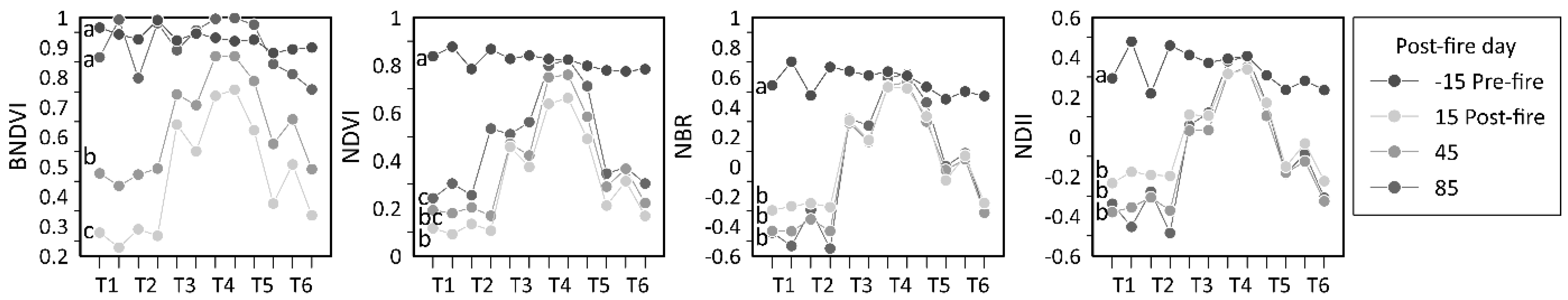
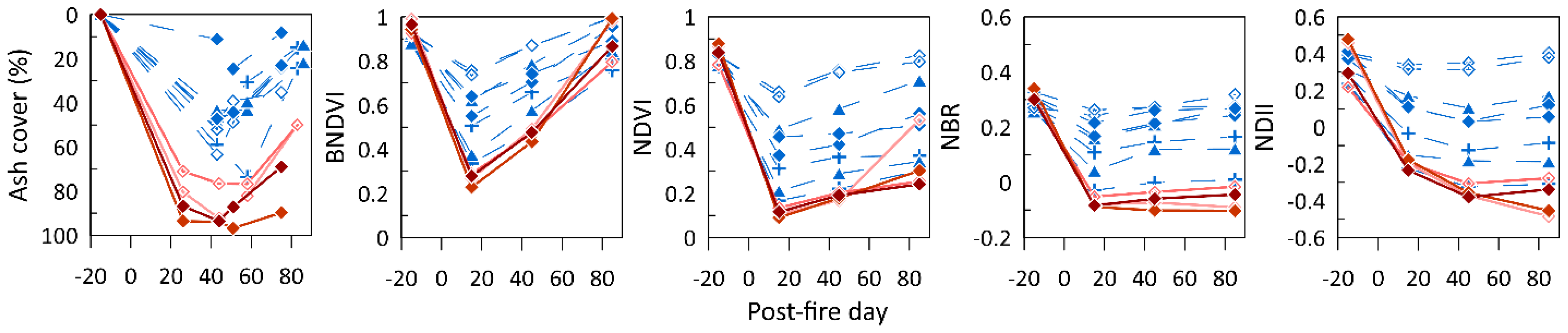
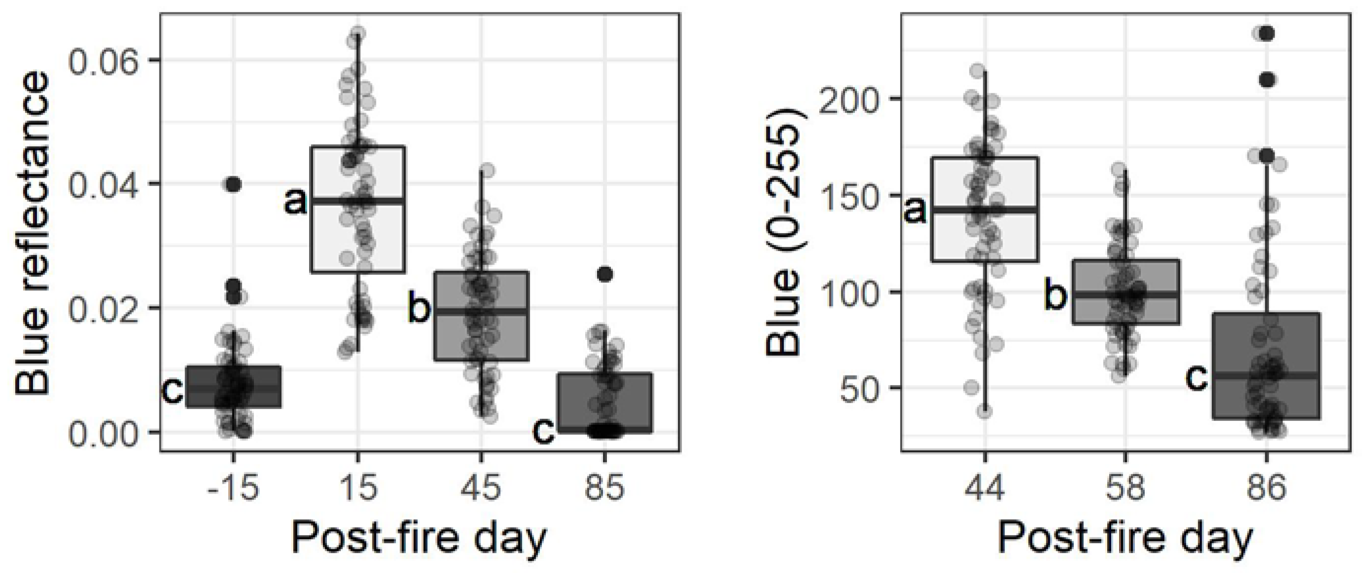
3.2. Spectral Band Analysis: Mesa Fire Plots

Sentinel (S2) bands’ reflectance was extracted at the Mesa Fire plot locations for each image date (Figure 6). The visible bands, namely the blue, green, and red bands, all showed an increase in reflectance immediately post-fire and then a decrease over time. The NIR band sharply decreased after the fire and remained fairly stable for the study duration. The SWIR bands more closely followed the pattern of the visible bands. It is the change in reflectance due to the fire (e.g., loss of green vegetation and increased soil and ash cover) that makes these bands suitable for post-fire mapping. Ratioing or differencing the NIR band (decrease due to fire) with a visible or SWIR band (increase due to fire) emphasizes this change.

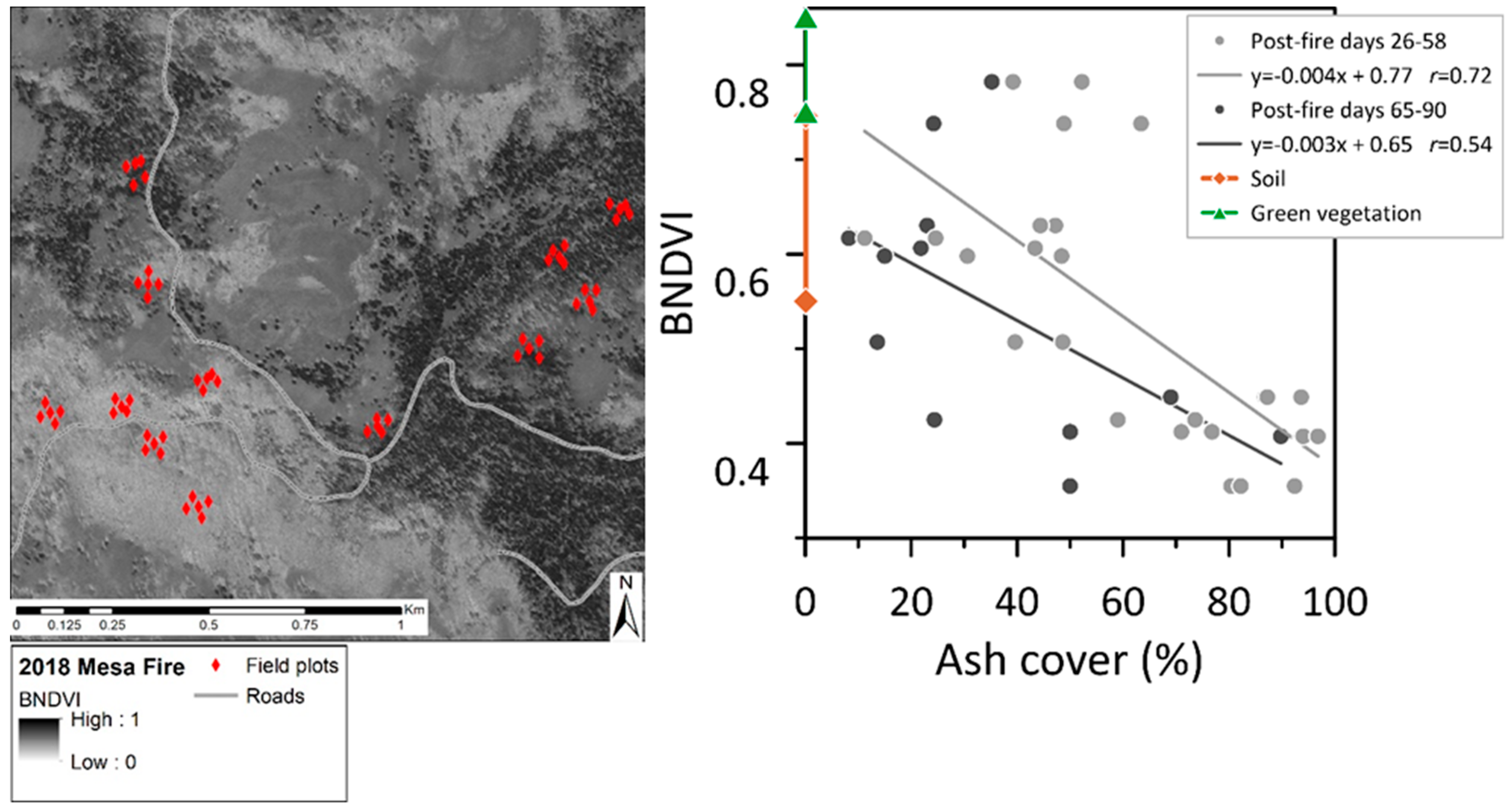
3.3. Disturbance Indices: Mesa Fire Plots

The pre-fire index values from the Mesa Fire are shown in dark gray and were higher across all plots and indices; these can be considered a baseline for pre-fire conditions (Figure 7). The first post-fire index values are in light gray, and for the BNDVI and NDVI, these values represent the greatest change from pre-fire values across all transects (Figure 7). For the NDII and NBR indices, the first post-fire values were indeed greatly lower than the pre-fire; however, the subsequent post-fire images from post-fire days 45–85 were nearly indistinguishable on most transects.

In the initial evaluation of these indices, it was important that: (1) there was a significant change from the pre to post-fire value; (2) the high and low/moderate severity plots were objectively distinguishable from each other based on index values; and (3) there was a notable recovery over time. All indices fit the first criteria: the dark line (pre-fire day 15) was markedly different from the post-fire image values. Transects T1 and T2 had the highest ash cover of all the plots and this is observable from the plots in Figure 5 and Figure 7 across all indices. This confirms that each of these indices are appropriate for post-fire mapping and identifying high-severity conditions, thus criteria 2 was met as well. However, unlike any of the other indices, BNDVI values changed substantially between each image date, showing a stair-step return towards the initial condition. The other indices were more clustered together over the post-fire image dates.

The results of the mixed models of the data in Figure 7 confirms that BNDVI was the only index that significantly differed between the initial (pre-fire day 15) and the first and second post-fire (post-fire days 15 and 45) image dates. By the final image date (post-fire days 85), the BNDVI values were not significantly different than the pre-fire values, indicating a trend towards the pre-fire conditions. Of all four indices evaluated in Figure 7, the BNDVI appears to best fit the third criteria we were assessing to map a “recovery” during the study period, as ash dissipated from the plots.

As disturbance indices, all four indices from the Mesa Fire data show notable deviations between the pre-fire and post-fire values (Figure 7 and Figure 8); however, BNDVI values indicate a gradual trend towards the pre-fire values over time in a way the other indices do not (Figure 8). The change in ash cover over time is included in Figure 8 for direct comparison. The shape of the disturbance curves of the BNDVI and ash cover plots are similar over the study period. We acknowledge that most broadband indices, particularly NDVI, were founded to evaluate vegetation (i.e., greenness), therefore it isn’t surprising that NDVI, for example, does not show a significant “recovery” in the first 90 post-fire days. The fire began in late July and the study progressed through the fall; substantial green-up would be expected the following spring. BNDVI has essentially the same index structure as NDVI, with the blue band ratioed with the NIR rather than the red band. Our data suggest that there is a meaningful change in the blue reflectance over time that is indicative of the ash and soil conditions we monitored in this study.

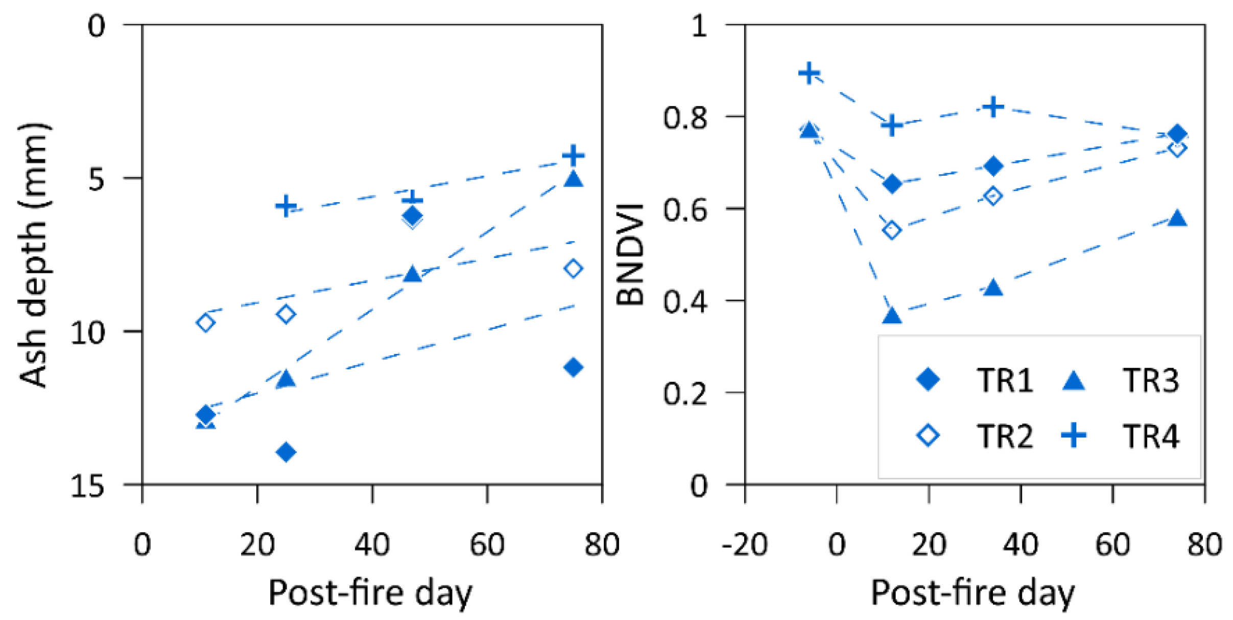
3.4. Redford Canyon Fire Pilot Study

To evaluate if the BNDVI may be suitable for mapping or monitoring ash more universally, we extended our analysis to include data from the 2017 Redford Canyon Fire. Field spectra of ash and ash–char–soil mixes were collected (Figure 9). The light gray ash is representative of ash shortly after a fire prior to wetting or redistribution. The continuum of light ash to dark ash to char–soil mixes represent ash over time as it becomes incorporated into the soil layers, as well as represents levels of combustion: a light ash color indicates complete organic combustion, while a darker ash color or char often reveals incomplete organic combustion. As expected, the uncharred soil had the highest reflectance, followed by the light gray ash, and then the reflectance generally decreased as the soil fraction of the soil–ash and soil–char mix increased. This is useful information because it confirms the decrease in reflectance over the full spectral region, not just in the visible region. The reflectance values were extracted at visible and NIR wavelengths (Figure 9), and these values were used to evaluate if a NIR/blue band ratio (as used in BNDVI) may be more indicative of ash than an NIR/red ratio (NDVI). Although the overall reflectance of ‘dark char soil’ was lower than that of ‘light ash’ or ‘soil’ (Figure 9), the ratio of the reflectance in the NIR region to the blue (e.g., NIR/Blue) was lowest for the ‘light ash’ (0.23/0.14 = 1.6), followed by ‘dark char soil’ (0.06/0.03 = 2.0) and ‘soil’ (0.33/0.15 = 2.2). This is why the BNDVI was lowest for the lightest colored ash (0.24) and increased with darker colored ash or char (0.33), and also over time as ash was incorporated into the soil (0.38). The reflectance of the blue band was higher relative to the NIR band with a lighter colored ash.

Similar to the Mesa Fire, BNDVI values from Redford Canyon Sentinel-2 imagery decreased immediately after the fire and increased steadily over the first 80 post-fire days (Figure 10). The plots with the deepest ash (e.g., TR3) and likely the highest ash cover had the lowest BNDVI values. All plots in this fire were classified as moderate-burn severity, thus the BNDVI values were higher overall than at the Mesa Fire in the 80-day post-fire period.

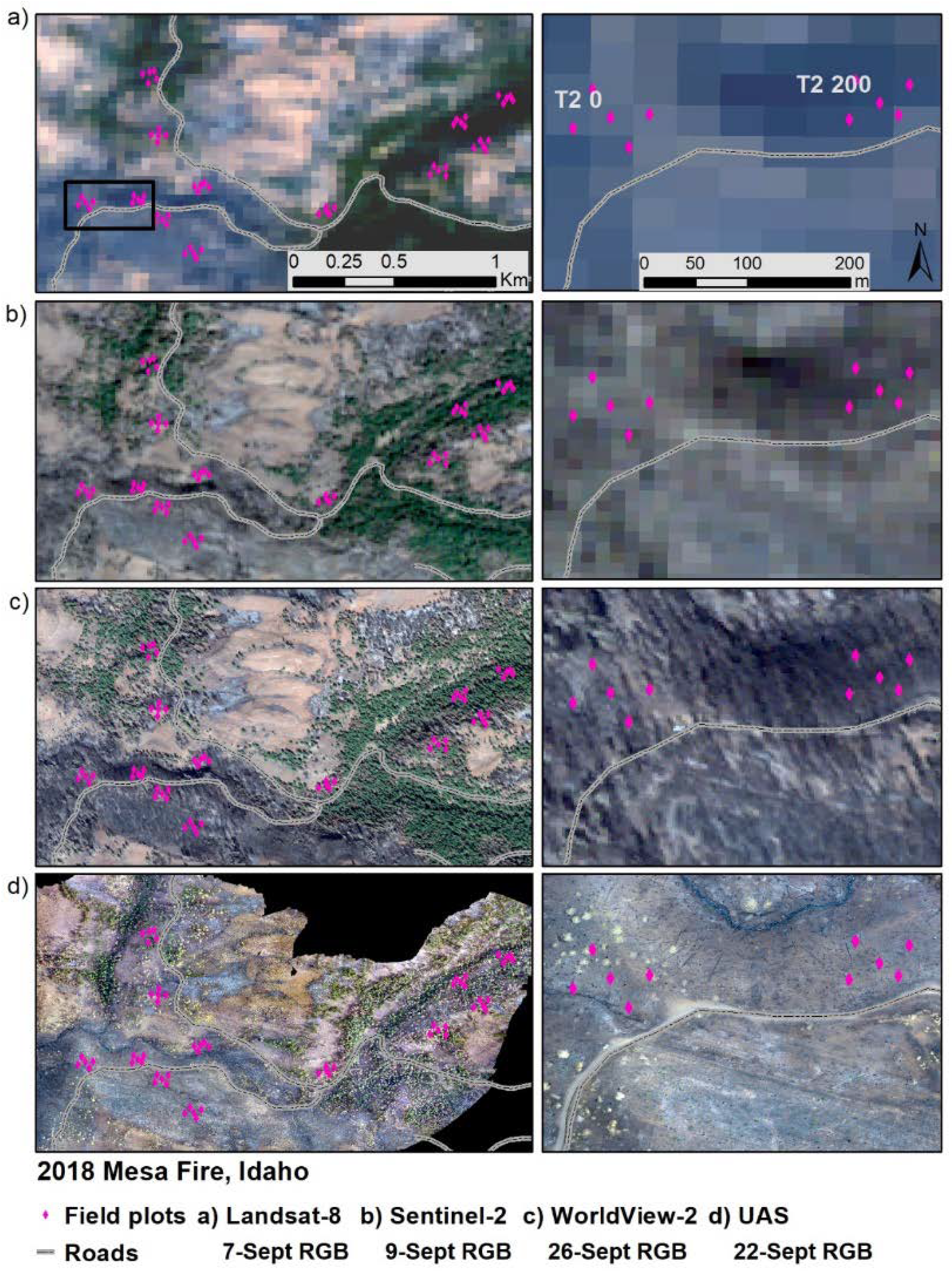
3.5. Comparing Imagery after the Mesa Fire

The images in Figure 11 are ordered by increasing spatial resolutions from Landsat (30 m pixels) at the top (a) to the UAS imagery with 0.6 m pixels at the bottom (d). At the full-scale (left column), all four image types appear to provide the same basic visual information: areas of green vegetation and the soil, ash, and char mix. However, when zoomed in to a single transect, the additional spatial information that the higher resolution imagery provides becomes clearly apparent. It is only at the 2 m scale of the WV2 imagery that tree crowns are visible and much finer features, such as fallen trees and stumps, ash patches, a small stream, road pullouts, and a field vehicle, are all recognizable. The UAS imagery improves upon the visible resolution of the satellite WV2 imagery and provides a clear picture of the ground conditions. Although three images were collected with the UAS, they were increasingly plagued by shadows as the season progressed and it was difficult to calibrate between images (i.e., light balancing, atmospheric conditions, and sun angle), which made higher-level processing untenable.

3.6. Mesa Fire UAS Image

The camera mounted on the UAS only collected RGB bands, which limits much of the image analysis that can be done with the reflectance imagery. The RGB values were also scaled at 0–255 (rather than at 0–1 for reflectance for satellite imagery). However, after discovering the relationship between the blue band and ash cover over time, we compared the change in blue reflectance between the S2 imagery and the UAS during the study period (Figure 12). The pattern of significant reflectance decrease in the first 90 post-fire days was statistically similar between the two sets of data. This may indicate that the addition of an NIR band (available on many UAS-mounted systems) could provide an ultra-high resolution ash cover map via the BNDVI.

3.7. Mesa Fire WorldView-2 Image

We calculated the BNDVI from a single-date WV2 image (26 September; post-fire day 62). The ash cover from 3–4 field visits to each plot were subset into two groups corresponding to pre and post- WV2 image collection to evaluate the time period(s) in which the field data correlated to the WV2 BNDVI values (Figure 13). The correlation coefficients (r) were only significant for the early time period (p < 0.001). The most notable difference between the two regression lines was the intercept, while the slopes remained largely unchanged between time periods. The earlier set of field data represents ash pre-rainfall (post-fire days 26–58), while the later set was measured after significant rainfall (days 65–90). Over the course of the study, most transects lost ~30% ash cover (Figure 5), which roughly corresponds to the difference in the x-axis values (ash cover) for a given BNDVI value. For a control or unburned reference, typical BNDVI values from soil and green vegetation are shown on the y-axis on the graph. As ash cover decreased over time on the burned plots, the BNDVI values approached those of uncharred soil. Other high BNDVI values on this figure are likely from areas that were lower-burn severity and had partial green canopy above the plot that influenced the pixel reflectance.

3.8. Mesa Fire Landsat Data

Landsat imagery provided essentially the same spectral information as Sentinel, with the major difference concerning the spatial resolution (pixel size: Landsat 30 m compared to 10 m Sentinel). Sentinel is also available on a higher temporal frequency, but in this study, we looked only at one image per month for both L8 and S2. We expected BNDVI calculated from L8 to be similar to that calculated from S2 (Pearson correlation, r = −0.57) but were somewhat surprised to find stronger correlations between Landsat data and the field data (r = −0.82). From strictly a correlation perspective, Landsat BNDVI values were more strongly correlated to the ash cover data. However, from a mapping perspective (Figure 11), it is clear that if S2 data is available, the additional spatial detail it can provide should be advantageous.

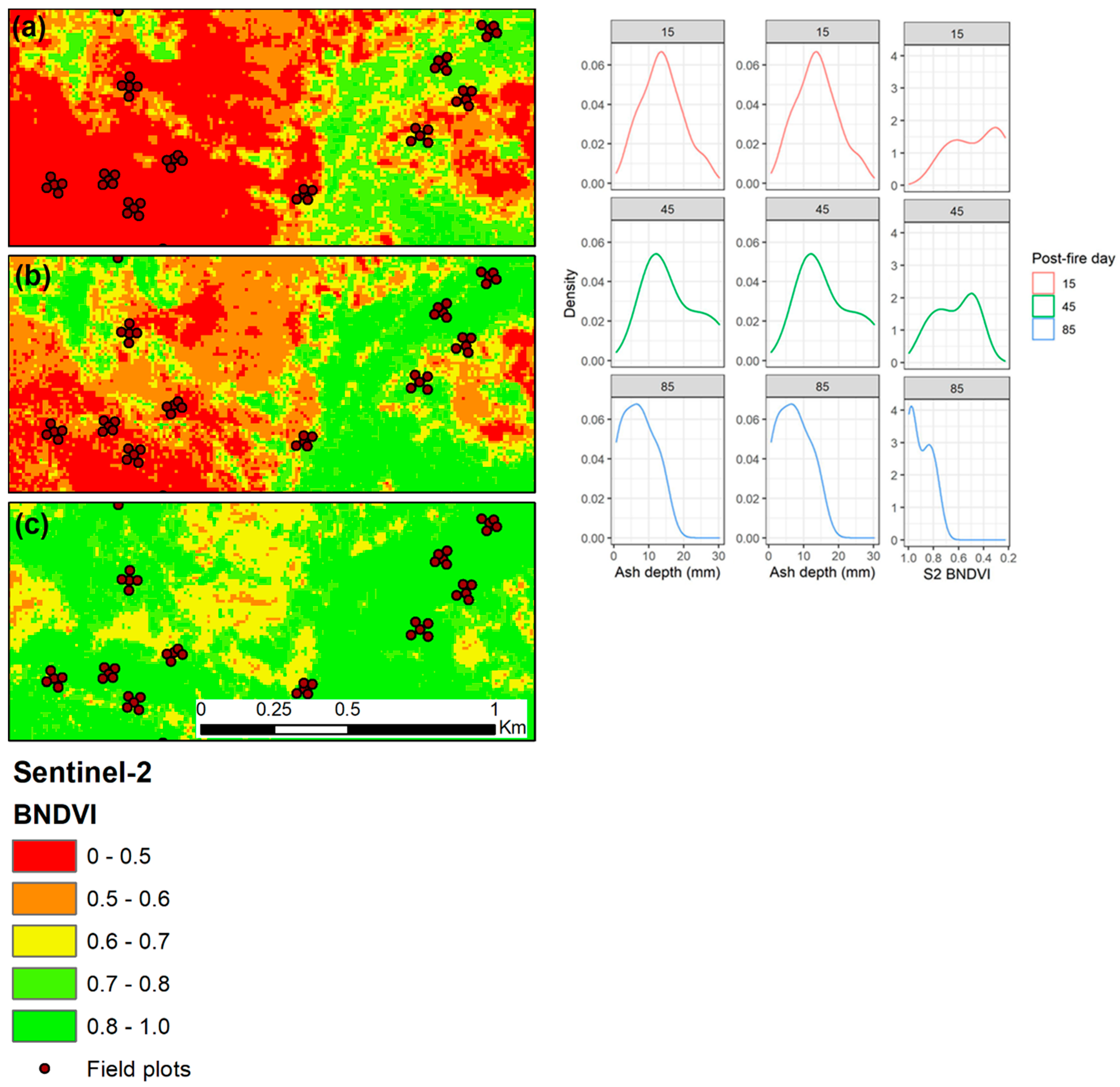
3.9. Mesa Fire Classified Sentinel-2 Time Series

The Sentinel-2 BNDVI data were classified as follows: BNDVI values less than 0.5 corresponded to ash cover greater than 60%, which can be considered high ash cover; BNDVI values between 0.5 and 0.7 indicated more moderate ash cover in the range of 40–60%; and BNDVI values greater than 0.7 were low ash cover (likely scattered ash cover where present) trending towards green vegetation or other unburned covers. From the time series of classified S2 images (Figure 14), it is possible to see how the ash cover in the area around the plots changed over time. The density distribution graphs of the ash cover, depth, and BNDVI values from the field plots concur with the classified images. Ash cover and depth decreased over time, while BNDVI values increased.

A linear mixed-effects model validated that the significant change in ash cover over time was mappable as a function of BNDVI, time, and burn severity (

Table 4. Results of the linear mixed-effects model (Ash cover = BNDVI ⸰ post-fire day ⸰ burn severity). Significant differences in the least-squared means between the post-fire day and severity groups are indicated by different letter groups (p < 0.05).

Post-Fire Day	Burn Severity	Ash Cover Estimate (%)	Standard Error	Letter Group
15		71	6.7	a
45		69	4.6	a
85		48	5.5	b
	High	82	5.4	a
	Low/moderate	32	4.0	b

). The significant decrease in ash cover between the post-fire days 45 and 85 was seen on all plots and was due to the nearly 40 mm of rainfall that was recorded in that period. The striking difference between the ash cover on the high and low severity plots was also significant, with about 2.5 times more ash cover on the high-severity plots throughout the study period. This is important from a mapping and modeling perspective, as it is more important to be able map and predict the areas that are of the greatest risk, which, in this study, are the areas with the highest ash cover and subsequently an elevated risk of post-fire runoff, soil and ash erosion, and water contamination.

4. Discussion

4.1. Change in Ash over Time

Ash cover and depth decreased over the study period regardless of the initial conditions or burn severity. The two high severity transects, Mesa Fire T1 and T2, had around 80% average ash cover at the time of the first sampling on post-fire day 26. Ash cover on these transects remained higher than the low/moderate transects through the entire study period, while ash depth decreased to nearly negligible levels on all plots. Ash cover decreased on all transects at about the same rate, while ash depth change was more variable depending on the initial ash depths (Figure 5). Determining ash cover is a subjective practice (see Figure 4); it is easier to quantify when it is light-colored and distinct from the underlying soil layers. As ash is redistributed by wind and water, and is incorporated into the soil below, it is increasingly difficult to distinguish from soil [18]. Measuring ash depth is less subjective; a flat-bottomed ruler was used to take several measurements at each plot and it is usually obvious by the change in texture and density when the ruler has hit soil. By the end of the study period, most plots had reached 0–5 mm of depth on average, even if there was observable ash cover. Considering we are defining ash as all combusted organic material that is mobile through the force of wind or water, it is often necessary to differentiate ash and soil by feeling the texture. In order to limit subjectivity between field samplers, we calibrated between team members. As can be seen in Figure 5, ash cover and depth decreased fairly consistently over all transects, indicating that our sampling efforts were relatively uniform.

One of our objectives was to determine how long ash persists on site and how often ash should be sampled in order to capture its dissipation over time. In theory, one could take ash cover and depth measurements daily or weekly, but that is generally not possible in practice. Our early field sampling dates were 2 weeks apart, progressing to about 4 weeks by the end of the study. This timing captured the gradual decline in ash cover and depth, with the biggest changes occurring as a result of rainfall, which was also found in [27]. Due to diligent monitoring, we were able to sample shortly after each precipitation event. Similar timing and sampling protocols were followed at both the Mesa Fire site and the pilot study of the Redford Canyon Fire site, and the results were similar in that most ash was gone by 80–90 days post-fire. Both fires occurred in the late summer and had convective precipitation events in the fall that led to ash mobilization. In contrast, the 2020 Cameron Peak Fire in Colorado burned from mid-August through mid-December (https://inciweb.nwcg.gov/incident/6964/, accessed on 9 September 2021). Much of the burned area did not receive rainfall before snowfall and when the snow melted in the spring of 2021, the ash was mostly undisturbed (C. Rhodes, pers. comm.). However, in 2021, managers were still concerned about ash movement into drinking water reservoirs; thus, the ash will ultimately be displaced by wind or water, and the importance of mapping and modelling its transport is still critical. There were several large wildfires in western Oregon in the fall of 2020 that burned the source watersheds of the cities of Eugene and Salem, and our research team was tasked with watershed modelling with an emphasis on ash movement into drinking water supplies (City of Salem, OR, USA, wildfire complexes BAER teams, pers. comm). These real-world examples emphasize the need for informed and efficient ash mapping and modelling technology.

The relationship between ash cover and depth is not as robust as we had expected it to be (Figure 5). Although there is a non-significant correlation when all data are considered (r~0.2), when only the high-burn severity sites are evaluated, the correlation is significant (r = 0.7; p < 0.002). The spatial and temporal variability of both the cover and depth across transects, and the entire burned landscape make it difficult to predict depth from cover, but it is more predictable in areas of greater ash cover. The passive optical sensors that are onboard the satellites we investigated in this study are able to map ash cover, but depth is not perceptible strictly from an aerial viewpoint. Ideally, a strong relationship between ash cover and depth would allow one to infer depth and ash load from a known or predicted ash cover value. Perhaps the most important finding regarding the change in post-fire ash over time is the timeframe in which it is detectable and measurable on site and regarding the rainfall needed to initiate transport. Some degree of cover persisted on all transects throughout the study period, however, ash depth approached zero by 90 days (Figure 5). From Figure 2, we see that there was no precipitation until post-fire day 65 and the first rainfall events greater than 10 mm were on post-fire day 70 (12 mm) and 75 (15 mm). After post-fire day 75, cumulative rainfall was just under 40 mm. Ten-minute rainfall intensity was less than 10 mm h⁻¹ for all of these events, which is a relatively low intensity. From these data, it appears that ash movement is instigated by a 10 mm rainfall event and that 10–30 mm of ash can be completely removed by 40 mm of rain. Pereira et al. [27] found substantial ash movement with 80 mm of rainfall. Woods and Balfour [26] reported a return to ‘no ash’ runoff and sediment conditions by the spring after a fall wildfire in Montana, which fits the same time frame as we measured.

In addition to ash cover and depth measurements, a composite ash sample was collected in a 400 cm² frame, which was oven-dried and weighed, and the ash bulk density was calculated in the lab for the three highest severity transects (Table 3). As emphasized in the introduction, the WATAR hydrologic model that is used to predict ash transport requires ash load (mass per area) as an input [24]. From the ash cover, depth, and weight data, we can calculate an ash load for each transect; similarly, we can also do this using the calculated bulk density. The difficult or inexact part of these calculations is in the composition of the field ash samples. The field samples contain mostly ash; however, soil, small rocks, and uncharred organics are inevitably inside the samples, rendering the weights questionable. From the field weights (data not shown), the ash bulk density ranged from 0.4 to 3.2 g·cm⁻³ (mean 1.2 g·cm⁻³) compared to our “pure” sieved ash sample bulk density of 0.3–0.4 g·cm⁻³ (Table 3). Calculating ash load with a bulk density of 0.3 g·cm⁻³ and a depth of 1 cm of ash at 60% cover yields 72 g of ash, while the same calculations with a bulk density of 1.2 g·cm⁻³ yields 288 g of ash, 400% more for the same area. We are emphasizing these discrepancies to bring attention to the variability inherent when using real data to build models.

4.2. Spectral Bands and Indices

Many other researchers have mapped post-fire ash, char, and soil burn severity [18,30,32,33,34,58,59]. However, our questions were focused on the timing of the ash mapping, the temporal persistence of ash, and the level of measurement precision necessary to reliably quantify ash. We were also interested in pursuing multiple mapping platforms with their inherent spatial and spectral differences, with the goal of an operational methodology that was practical to be implemented multiple times in a short timeframe. Thus, our spectral band and spectral index analysis were not solely influenced by the strongest relationship with ash at any given point. Instead, we needed a mapping method that fit several criteria: that it (1) detected a significant change between pre and post-fire conditions; (2) portrayed a notable recovery towards the pre-fire condition that matched the temporal change in ash; and (3) had the ability to distinguish between high and low ash cover. Soil burn severity is often mapped after wildfires to determine which areas are at the highest risk for runoff or soil erosion [19,28,60], and abundant bare soil (lacking protective organic cover) over more than 60% of the area is often a threshold for increased erosion potential [61]. Similarly, we found a natural breakpoint in the ash cover data, indicating that more than 60% of the ash was classified as high ash cover. A map was created using classified BNDVI values (Figure 14), highlighting areas that had greater than 60% ash cover and expressed the change in ash cover over time.

While not especially common in vegetative or burned area indices, the blue spectral region has been associated with accounting for atmospheric effects when used as a burned area index [55]. The Landsat and Sentinel satellite imagery evaluated in this study were corrected to the surface reflectance or bottom of the atmosphere (BOA) reflectance, while the WorldView imagery was corrected with a dark object subtraction. Both corrections were implemented to minimize atmospheric effects during analyses. The BNDVI rather than the NDVI is sometimes used when crop mapping with aerial imagery that is difficult to atmospherically correct. Others have mapped burned vegetation as well as vegetation conditions using the BNDVI [62,63]. Ngadze et al. [64] found that the NIR and blue bands of L8 and S2 contributed most to burned-area detection over two study sites over a savannah landscape in Zimbabwe. Our working theory is that ash and char can reflect gray, which is in the blue spectral region, and the absence of green vegetation is detectable with the BNDVI. Indeed, it appears that there is a greater change between the pre and post-fire blue rather than red values on the ash-covered plots (Figure 9), and that the blue values return almost to the pre-fire condition by the end of the study (Figure 6 and Figure 12). Many of the indices we evaluated initially were correlated with the post-fire ash cover, yet only the BNDVI reflected the return to pre-fire conditions in the 90-day study period (Figure 7). Additionally, the similar relationship between ash cover and BNDVI over time on two fires is encouraging for further investigation in other post-fire environments.

Ash mapping using the BNDVI fits within the operational goal of this study. The blue and NIR bands are available on all EO satellites. SWIR bands are also generally available, albeit at a coarser spatial resolution (30 m on Landsat and 20 m on Sentinel). Thus, a valid concern is the loss of spatial resolution. Looking at the ash cover photo series of the post-fire days (Figure 4), the very fine-scale variability of the post-fire conditions is apparent. While it is not practical, nor is it likely necessary to map ash (or other post-fire attributes) at the sub-meter scale (as with a UAS), the loss of information with too large of a pixel is a concern (as with Landsat) [32]. Patches of ash would need to be large (>60 m) to be detectable at the 30 m scale of L8 imagery. While Landsat and Sentinel images are commonly used in post-fire mapping, the tradeoff is in the ability to map a large area very quickly without a huge data cost, with the assumption of some loss of detailed ground information [65]. NBR is a common burned area index [36] and has been used successfully to map char [9,31,66]. The NDII is the basis for the ash load index Chafer et al. [34] developed to successfully map ash in Australia. Both of these established indices utilize SWIR bands because of the significant change in pre to post-fire reflectance that highlights the loss of vegetation and the increase in both soil and other non-organic covers.

For this study, we deliberately chose to not do higher-level analysis, such as spectral unmixing [30,33,66], fusion of multiple data layers [67], or data mining of our suite of field and image data [64]. Within the time constraints of post-wildfire severity assessment and hydrologic modelling predictions, there is not always time for more complex analysis techniques. Satellite imagery is collected repeatedly as it is available and the first cloud- and smoke-free image that captures the entirety of the burned area is used by land managers to evaluate the condition of the burned area and guide mitigation decisions. The timeline is generally “as-soon-as-possible” and is almost always accomplished within 2 weeks of fire control. The 2-week window has historically been tied to the availability of Landsat satellite data, which has a return period of 16 days; in recent years, post-fire maps have started using Sentinel data with its 5-day return period. The burn severity mapping protocol is widely accepted and highly standardized, and can be accomplished quickly without extensive expertise [28]. A key goal of this study was to evaluate a similar methodology for ash cover that was reproducible and could eventually be made operational. The recent surge of UAS technology and accessibility is also likely to alter the post-fire mapping arena [38,39,68]. Imagery will be available within hours, not days, and the image resolution (spatial scale) will be very fine. UASs often have cameras with visible bands and many have an NIR band as well (far fewer have SWIR bands). An ash map created with BNDVI would be reproducible on any imaging platform that has an NIR band, allow more flexibility regarding the decision for spatial or timing considerations.

4.3. Considerations and Decision-Making Tool

There is a cost–benefit evaluation that must be done when deciding which imagery to use for post-fire mapping (

Table 5. Post-wildfire ash mapping cost–benefit considerations with image extent approximately normalized to 100 km².

Platform/Satellite		Bands Used (as Available)	Acquisition/Return Period	Cost per 100 km2	Time to Process	Area and Specifications	Data Volume
UAS	Specs:	RGB (NIR)	As collected	$16,000 1 (16 days)	Days	4 km2 3-band	Ultra-high (1.5 GB)
	Pros:	+ very high spatial resolution + easily interpretable by novice + becoming more mainstream + safer than in-person reconnaissance in a post-fire environment
	Cons:	high data volume specialized processing equipment limited data analysis costly and time intensive to collect expensive to contract for both collection and processing
World View-2	Specs:	RGB/NIR (SWIR on WV-3)	Tasked/as ordered	$2500	Hours	100 km2 orthorectified 4-band	Moderate (300 MB)
	Pros:	+ high spatial resolution + availability of NIR band + moderate data volume + can be tasked to area of interest within days
	Cons:	moderately expensive to task no automatic collection need for orthorectification and atmospheric correction
Sentinel-2	Specs:	RGB/NIR/SWIR	Automatic/5–10 days	Free	Hours	100 km2 orthorectified 12-band	Moderate (600–800 MB)
	Pros:	+ moderate spatial resolution + weekly automatic collection + high current interest by researchers and scientists + availability of data management and processing scripts in R and Python
	Cons:	images may be plagued by clouds or smoke moderate data volume necessitates resampling of area of interest
Landsat-8	Specs:	RGB/NIR/SWIR	Automatic/16 days	Free	Hours	300 km2 orthorectified 11-bands	Moderate (900+ MB)
	Pros:	+ benchmark standard of post-fire mapping + repeatable and reliable + near-automatic processing for many applications + bi-monthly return period
	Cons:	lowest spatial resolution of image in this study in general, too coarse to capture the variability and change in post-fire ash over time

¹ This is an approximate fair-market value of the past 2 years (~$1000/day). This cost can vary widely, especially as UAS ownership and instrument availability increase.

). Considerations include image or platform availability, timing, cost, and spectral and spatial resolution [69]. Less tangible factors involve the practical application or operational implementation of a particular technology. For time-sensitive image collection and rapid data needs, the chosen technology needs to be available, reliable, and consistent.

Benefits of L8, S2, and WV2 data include consistency in the data products. Each scene is collected in a single or small number of multiple tile(s) at a consistent elevation and sun angle per tile. This makes processing across images, combining and mosaicking images, and time-series analysis practical, and the derived data products generally have a high level of accuracy [70]. This is more difficult with a UAS but can be accomplished with very consistent flight plans and data collection [41].

UAS imagery is often very high resolution; however, collection logistics are time-consuming and have more room for error in terms of elevation, angle, cloud cover, shadows, mechanical breakdown, and camera issues. The image acquisition time using a UAS can also be considerable. For instance, the minimum area that can be tasked (ordered) for WV2 imagery is 100 km² (10,000 ha); it would take multiple days or multiple instruments to image that area via UAS. WV2 has a sun-synchronous orbit, data collections are illuminated, and it can collect 1 million km² per day (https://resources.maxar.com/data-sheets/worldview-2, accessed on 13 September 2021). S2 tiles are also 100 km² and L8 tiles are even bigger (180 km²), and both have the benefit of being a single file, which makes processing more streamlined. Data volume is a consideration for data management as well as for processing time. For example: the 8 September UAS image at its native 0.06 m resolution is 1.5 GB of data in a three-band file (Table 5). Resampled to 2 m via bilinear resampling, the data volume is reduced to 16.5 MB. Each operation on the full resolution image took 30–60 min while processing the 2 m file and operations were << 1 min long.

The pros and cons in Table 5 are applicable for other post-fire (or other disturbance) mapping considerations. Managers and data scientists need to prioritize their image needs as well as and time and financial constraints when selecting an imaging platform. We also acknowledge that oftentimes it is solely an availability issue, and for that reason, we have presented a case for mapping ash with several different platforms with reasonable success. As a final recommendation, however, for the goals of this study, Sentinel-2 seems to best-suited for mapping ash over time when the eventual next step is to incorporate the results into other models.

5. Conclusions

Post-wildfire ash cover and depth were evaluated from multiple platforms at various spatial and temporal scales, and we found that ash persisted onsite with little change until the first significant rainfall event (10 mm). Several other low intensity rain events in the first 90 post-fire days resulted in most of the ash being removed from the burned areas. Two high-burn severity field transects had 70–80% ash cover initially, while the remaining mixed low and moderate burn severity transects started with 50–60% ash cover. Ash depths were more variable and ranged from 5 to 30 mm initially, decreased to 0–5 mm, and were not as dependent on burn severity. Since ash depth was less than 5 mm after 80–90 days, the risk of transportable ash decreased to a negligible degree.

We demonstrated relationships between the ash cover and several common vegetation and post-fire spectral indices, but the one that most closely fit the trend of the change in ash cover over the study period was the blue normalized difference vegetation index (BNDVI). The BNDVI time series matched the ash cover and depth trends over 90 days. Additionally, we found that a practical resolution for mapping ash was with either 2 m pixels (WV2) or 10 m (S2). Pixels in this range captured the variability of the ground conditions while also ensuring that the data volume and analysis time ‘cost’ were manageable. A monthly time scale was appropriate to monitor the change in ash, particularly since rain events seemed to be the primary driving force for mobilizing the ash. In terms of spectral resolution (available wavebands), WV2, S2, and L8 all have the necessary visible and NIR bands for creating time series ash maps with BNDVI. Therefore, the Sentinel-2 imagery best fit the criteria because the data are free; are available every 5 days; the data volume of the 10 m pixels are reasonable to manage; and its accessibility and formatting would easily lend itself to moving towards operational methodologies that could be used for post-fire hydrologic modelling.

References

1. Westerling, A.L.; Hidalgo, H.G.; Cayan, D.R.; Swetnam, T.W. Warming and earlier spring increase western US forest wildfire activity. Science 2006, 313, 940–943. [Google Scholar] [CrossRef] [Green Version]
2. Keane, R.E. Cascading Effects of Fire Exclusion in Rocky Mountain Ecosystems: A Literature Review; General Technical Report RMRS; U.S. Department of Agriculture, Forest Service, Rocky Mountain Research Station: Ft. Collins, CO, USA, 2002; pp. 1–24. [CrossRef] [Green Version]
3. Pechony, O.; Shindell, D.T. Driving forces of global wildfires over the past millennium and the forthcoming century. Proc. Natl. Acad. Sci. USA 2010, 107, 19167–19170. [Google Scholar] [CrossRef] [PubMed] [Green Version]
4. Kabisch, N.; Selsam, P.; Kirsten, T.; Lausch, A.; Bumberger, J. A multi-sensor and multi-temporal remote sensing approach to detect land cover change dynamics in heterogeneous urban landscapes. Ecol. Indic. 2019, 99, 273–282. [Google Scholar] [CrossRef]
5. Rhoades, C.C.; Nunes, J.P.; Silins, U.; Doerr, S.H. The influence of wildfire on water quality and watershed processes: New insights and remaining challenges. Int. J. Wildl. Fire 2019, 28, 721–725. [Google Scholar] [CrossRef] [Green Version]
6. Moody, J.A.; Martin, D.A. Synthesis of sediment yields after wildland fire in different rainfall regimes in the western United States. Int. J. Wildl. Fire 2009, 18, 96–115. [Google Scholar] [CrossRef]
7. Shakesby, R.A.; Doerr, S.H. Wildfire as a hydrological and geomorphological agent. Earth Sci. Rev. 2006, 74, 269–307. [Google Scholar] [CrossRef]
8. Robichaud, P.R.; Wagenbrenner, J.W.; Brown, R.E. Rill erosion in natural and disturbed forests: 1. Measurements. Water Resour. Res. 2010, 46, 1–14. [Google Scholar] [CrossRef]
9. Smith, A.M.S.; Eitel, J.U.H.; Hudak, A.T. Spectral analysis of charcoal on soils: Implicationsfor wildland fire severity mapping methods. Int. J. Wildl. Fire 2010, 19, 976–983. [Google Scholar] [CrossRef]
10. Smith, A.M.S.; Hudak, A.T. Estimating combustion of large downed woody debris from residual white ash. Int. J. Wildl. Fire 2005, 14, 245–248. [Google Scholar] [CrossRef] [Green Version]
11. Hudak, A.T.; Ottmar, R.D.; Vihnanek, R.E.; Brewer, N.W.; Smith, A.M.S.; Morgan, P. The relationship of post-fire white ash cover to surface fuel consumption. Int. J. Wildl. Fire 2013, 22, 780–785. [Google Scholar] [CrossRef]
12. Brewer, N.W.; Smith, A.M.S.; Hatten, J.A.; Higuera, P.E.; Hudak, A.T.; Ottmar, R.D.; Tinkham, W.T. Fuel moisture influences on fire-altered carbon in masticated fuels: An experimental study. J. Geophys. Res. Biogeosci. 2013, 118, 30–40. [Google Scholar] [CrossRef] [Green Version]
13. Onda, Y.; Dietrich, W.E.; Booker, F. Evolution of overland flow after a severe forest fire, Point Reyes, California. Catena 2008, 72, 13–20. [Google Scholar] [CrossRef]
14. Larsen, I.J.; MacDonald, L.H.; Brown, E.; Rough, D.; Welsh, M.J.; Pietraszek, J.H.; Libohova, Z.; Benavides-Solorio, J.D.D.; Schaffrath, K. Causes of post-fire runoff and erosion: Water repellency, cover, or soil sealing? Soil Sci. Soc. Am. J. 2009, 73, 1393–1407. [Google Scholar] [CrossRef] [Green Version]
15. Woods, S.W.; Balfour, V.N. The effects of soil texture and ash thickness on the post-fire hydrological response from ash-covered soils. J. Hydrol. 2010, 393, 274–286. [Google Scholar] [CrossRef]
16. Balfour, V.N.; Doerr, S.H.; Robichaud, P.R. The temporal evolution of wildfire ash and implications for post-fire infiltration. Int. J. Wildl. Fire 2014, 23, 733–745. [Google Scholar] [CrossRef] [Green Version]
17. Balfour, V.N.; Woods, S.W. The hydrological properties and the effects of hydration on vegetative ash from the Northern Rockies, USA. Catena 2013, 111, 9–24. [Google Scholar] [CrossRef]
18. Santín, C.; Doerr, S.H.; Otero, X.L.; Chafer, C.J. Quantity, composition and water contamination potential of ash produced under different wildfire severities. Environ. Res. 2015, 142, 297–308. [Google Scholar] [CrossRef] [Green Version]
19. Robichaud, P.R.; Lewis, S.A.; Wagenbrenner, J.W.; Brown, R.E.; Pierson, F.B. Quantifying long-term post-fire sediment delivery and erosion mitigation effectiveness. Earth Surf. Process. Landf. 2020, 45, 771–782. [Google Scholar] [CrossRef]
20. Bodí, M.B.; Martin, D.A.; Balfour, V.N.; Santín, C.; Doerr, S.H.; Pereira, P.; Cerdà, A.; Mataix-Solera, J. Wildland fire ash: Production, composition and eco-hydro-geomorphic effects. Earth Sci. Rev. 2014, 130, 103–127. [Google Scholar] [CrossRef]
21. Burton, C.A.; Hoefen, T.M.; Plumlee, G.S.; Baumberger, K.L.; Backlin, A.R.; Gallegos, E.; Fisher, R.N. Trace elements in stormflow, ash, and burned soil following the 2009 station fire in Southern California. PLoS ONE 2016, 11, e0153372. [Google Scholar] [CrossRef]
22. Nunes, J.P.; Doerr, S.H.; Sheridan, G.; Neris, J.; Santín, C.; Emelko, M.B.; Silins, U.; Robichaud, P.R.; Elliot, W.J.; Keizer, J. Assessing water contamination risk from vegetation fires: Challenges, opportunities and a framework for progress. Hydrol. Process. 2018, 32, 687–694. [Google Scholar] [CrossRef] [Green Version]
23. Pereira, P.; Bogunovic, I.; Zhao, W.; Barcelo, D. Short-term effect of wildfires and prescribed fires on ecosystem services. Curr. Opin. Environ. Sci. Health 2021, 22, 100266. [Google Scholar] [CrossRef]
24. Neris, J.; Santin, C.; Lew, R.; Robichaud, P.R.; Elliot, W.J.; Lewis, S.A.; Sheridan, G.; Rohlfs, A.M.; Ollivier, Q.; Oliveira, L.; et al. Designing tools to predict and mitigate impacts on water quality following the Australian 2019/2020 wildfires: Insights from Sydney’s largest water supply catchment. Integr. Environ. Assess. Manag. 2021. [Google Scholar] [CrossRef]
25. Robinne, F.N.; Hallema, D.W.; Bladon, K.D.; Flannigan, M.D.; Boisramé, G.; Bréthaut, C.M.; Doerr, S.H.; Di Baldassarre, G.; Gallagher, L.A.; Hohner, A.K.; et al. Scientists’ warning on extreme wildfire risks to water supply. Hydrol. Process. 2021, 35, e14086. [Google Scholar] [CrossRef]
26. Woods, S.W.; Balfour, V.N. The effect of ash on runoff and erosion after a severe forest wildfire, Montana, USA. Int. J. Wildl. Fire 2008, 17, 535–548. [Google Scholar] [CrossRef]
27. Pereira, P.; Cerdà, A.; Úbeda, X.; Mataix-Solera, J.; Martin, D.; Jordán, A.; Burguet, M. Spatial models for monitoring the spatio-temporal evolution of ashes after fire—A case study of a burnt grassland in Lithuania. Solid Earth 2013, 4, 153–165. [Google Scholar] [CrossRef] [Green Version]
28. Parsons, A.; Robichaud, P.R.; Lewis, S.A.; Napper, C.; Clark, J.T. Field Guide for Mapping Post-Fire Soil Burn Severity; General Technical Report RMRS-GTR-243; U.S. Department of Agriculture, Forest Service, Rocky Mountain Research Station: Ft. Collins, CO, USA, 2010.
29. Miller, M.E.; Elliot, W.J.; Billmire, M.; Robichaud, P.R.; Endsley, K.A. Rapid-response tools and datasets for post-fire remediation: Linking remote sensing and process-based hydrological models. Int. J. Wildl. Fire 2016, 25, 1061–1073. [Google Scholar] [CrossRef]
30. Lewis, S.A.; Hudak, A.T.; Robichaud, P.R.; Morgan, P.; Satterberg, K.L.; Strand, E.K.; Smith, A.M.S.; Zamudio, J.A.; Lentile, L.B. Indicators of burn severity at extended temporal scales: A decade of ecosystem response in mixed-conifer forests of western Montana. Int. J. Wildl. Fire 2017, 26, 755–771. [Google Scholar] [CrossRef] [Green Version]
31. Hudak, A.T.; Morgan, P.; Bobbitt, M.J.; Smith, A.M.S.; Lewis, S.A.; Lentile, L.B.; Robichaud, P.R.; Clark, J.T.; Mckinley, R.A. The relationship of multispectral satellite imagery. Fire Ecol. 2007, 3, 64–90. [Google Scholar] [CrossRef]
32. Kokaly, R.F.; Rockwell, B.W.; Haire, S.L.; King, T.V.V. Characterization of post-fire surface cover, soils, and burn severity at the Cerro Grande Fire, New Mexico, using hyperspectral and multispectral remote sensing. Remote Sens. Environ. 2007, 106, 305–325. [Google Scholar] [CrossRef]
33. Robichaud, P.R.; Lewis, S.A.; Laes, D.Y.M.; Hudak, A.T.; Kokaly, R.F.; Zamudio, J.A. Postfire soil burn severity mapping with hyperspectral image unmixing. Remote Sens. Environ. 2007, 108, 467–480. [Google Scholar] [CrossRef] [Green Version]
34. Chafer, C.J.; Santín, C.; Doerr, S.H. Modelling and quantifying the spatial distribution of post-wildfire ash loads. Int. J. Wildl. Fire 2016, 25, 249–255. [Google Scholar] [CrossRef] [Green Version]
35. Key, C.H.; Benson, N.C. Landscape Assessment (LA) Sampling and Analysis Methods; General Technical Report RMRS-GTR-164-CD; U.S. Department of Agriculture, Forest Service, Rocky Mountain Research Station: Ft. Collins, CO, USA, 2006.
36. Chafer, C.J. A comparison of fire severity measures: An Australian example and implications for predicting major areas of soil erosion. Catena 2008, 74, 235–245. [Google Scholar] [CrossRef]
37. Lentile, L.B.; Holden, Z.A.; Smith, A.M.S.; Falkowski, M.J.; Hudak, A.T.; Morgan, P.; Lewis, S.A.; Gessler, P.E.; Benson, N.C. Remote sensing techniques to assess active fire characteristics and post-fire effects. Int. J. Wildl. Fire 2006, 15, 319–345. [Google Scholar] [CrossRef]
38. Stavros, N.E.; Agha, A.; Sirota, A.; Quadrelli, M.; Ebadi, K.; Yun, K. Smoke sky–Exploring new frontiers of unmanned aerial systems for wildland fire science and applications. arXiv 2019, arXiv:1911.08288. [Google Scholar]
39. Samiappan, S.; Hathcock, L.; Turnage, G.; McCraine, C.; Pitchford, J.; Moorhead, R. Remote sensing of wildfire using a small unmanned aerial system: Post-fire mapping, vegetation recovery and damage analysis in grand bay, Mississippi/Alabama, USA. Drones 2019, 3, 43. [Google Scholar] [CrossRef] [Green Version]
40. Hamilton, D.; Bowerman, M.; Colwell, J.; Donohoe, G.; Myers, B. Spectroscopic analysis for mapping wildland fire effects from remotely sensed imagery. J. Unmanned Veh. Syst. 2017, 5, 146–158. [Google Scholar] [CrossRef] [PubMed] [Green Version]
41. Xue, J.; Su, B. Significant remote sensing vegetation indices: A review of developments and applications. J. Sens. 2017, 2017, 1353691. [Google Scholar] [CrossRef] [Green Version]
42. Melville, B.; Fisher, A.; Lucieer, A. Ultra-high spatial resolution fractional vegetation cover from unmanned aerial multispectral imagery. Int. J. Appl. Earth Obs. Geoinf. 2019, 78, 14–24. [Google Scholar] [CrossRef]
43. Williams, C.K.; Kelley, B.F.; Smith, B.G.; Lillybridge, T.R. Forested Plant Associations of the Colville National Forest; General Technical Report PNW-GTR-36; US Department of Agriculture, Forest Service, Pacific Northwest Research Station: Portland, OR, USA, 1995.
44. Lentile, L.; Morgan, P.; Hardy, C.; Hudak, A.; Means, R.; Ottmar, R.; Robichaud, P.; Sutherland, E.K.; Szymoniak, J.; Way, F.; et al. Value and Challenges of Conducting Rapid Response Research on Wildland Fires; General Technical Report RMRS-GTR-193; U.S. Department of Agriculture, Forest Service, Rocky Mountain Research Station: Fort Collins, CO, USA, 2007.
45. Steinfeld, D.; Kern, J.; Gallant, G.; Riley, S. Monitoring roadside revegetation projects. Nativ. Plants J. 2011, 12, 269–275. [Google Scholar] [CrossRef]
46. Main-Knorn, M.; Pflug, B.; Louis, J.; Debaecker, V.; Müller-Wilm, U.; Gascon, F. Sen2Cor for Sentinel-2. In Image and Signal Processing for Remote Sensing XXIII; International Society for Optics and Photonics: Bellingham, WA, USA, 2017; p. 10427. [Google Scholar] [CrossRef] [Green Version]
47. Ranghetti, L.; Boschetti, M.; Nutini, F.; Busetto, L. “sen2r”: An R toolbox for automatically downloading and preprocessing Sentinel-2 satellite data. Comput. Geosci. 2020, 139, 104473. [Google Scholar] [CrossRef]
48. Fernández, C.; Fernández-Alonso, J.M.; Vega, J.A. Exploring the effect of hydrological connectivity and soil burn severity on sediment yield after wildfire and mulching. Land Degrad. Dev. 2020, 31, 1611–1621. [Google Scholar] [CrossRef]
49. Navarro, G.; Caballero, I.; Silva, G.; Parra, P.C.; Vázquez, Á.; Caldeira, R. Evaluation of forest fire on Madeira Island using Sentinel-2A MSI imagery. Int. J. Appl. Earth Obs. Geoinf. 2017, 58, 97–106. [Google Scholar] [CrossRef] [Green Version]
50. Roy, D.P.; Boschetti, L.; Trigg, S.N. Remote sensing of fire severity: Assessing the performance of the normalized burn ratio. IEEE Geosci. Remote Sens. Lett. 2006, 3, 112–116. [Google Scholar] [CrossRef] [Green Version]
51. Carlson, T.N.; Ripley, D.A. On the relation between NDVI, fractional vegetation cover, and leaf area index. Remote Sens. Environ. 1997, 62, 241–252. [Google Scholar] [CrossRef]
52. Escuin, S.; Navarro, R.; Fernández, P. Fire severity assessment by using NBR (Normalized Burn Ratio) and NDVI (Normalized Difference Vegetation Index) derived from LANDSAT TM/ETM images. Int. J. Remote Sens. 2008, 29, 1053–1073. [Google Scholar] [CrossRef]
53. Fernández-Manso, A.; Fernández-Manso, O.; Quintano, C. SENTINEL-2A red-edge spectral indices suitability for discriminating burn severity. Int. J. Appl. Earth Obs. Geoinf. 2016, 50, 170–175. [Google Scholar] [CrossRef]
54. Wang, F.; Huang, J.; Tang, Y.; Wang, X. New vegetation index and its application in estimating leaf area index of rice. Rice Sci. 2007, 14, 195–203. [Google Scholar] [CrossRef]
55. Mpakairi, K.S.; Kadzunge, S.L.; Ndaimani, H. Testing the utility of the blue spectral region in burned area mapping: Insights from savanna wildfires. Remote Sens. Appl. Soc. Environ. 2020, 20, 100365. [Google Scholar] [CrossRef]
56. Tucker, C.J. Red and photographic infrared linear combinations for monitoring vegetation. Remote Sens. Environ. 1979, 8, 127. [Google Scholar] [CrossRef] [Green Version]
57. Littell, R.C.; Milliken, G.A.; Stroup, W.W.; Wolfinger, R.D.; Oliver, S. SAS for Mixed Models, 2nd ed.; SAS Publishing: Cary, NC, USA, 2006; ISBN 1590475003. [Google Scholar]
58. Lentile, L.B.; Smith, A.M.S.; Hudak, A.T.; Morgan, P.; Bobbitt, M.J.; Lewis, S.A.; Robichaud, P.R. Remote sensing for prediction of 1-year post-fire ecosystem condition. Int. J. Wildl. Fire 2009, 18, 594–608. [Google Scholar] [CrossRef] [Green Version]
59. Van Wagtendonk, J.W.; Root, R.R.; Key, C.H. Comparison of AVIRIS and Landsat ETM+ detection capabilities for burn severity. Remote Sens. Environ. 2004, 92, 397–408. [Google Scholar] [CrossRef]
60. Robichaud, P.R.; Lewis, S.A.; Wagenbrenner, J.W.; Ashmun, L.E.; Brown, R.E. Post-fire mulching for runoff and erosion mitigation. Part I: Effectiveness at reducing hillslope erosion rates. Catena 2013, 105, 75–92. [Google Scholar] [CrossRef]
61. Pannkuk, C.D.; Robichaud, P.R. Effectiveness of needle cast at reducing erosion after forest fires. Water Resour. Res. 2003, 39, 1–9. [Google Scholar] [CrossRef]
62. Zou, X.; Haikarainen, I.; Haikarainen, I.P.; Mäkelä, P.; Mõttus, M.; Pellikka, P. Effects of crop leaf angle on LAI-sensitive narrow-band vegetation indices derived from imaging spectroscopy. Appl. Sci. 2018, 8, 1435. [Google Scholar] [CrossRef] [Green Version]
63. Estrany, J.; Ruiz, M.; Calsamiglia, A.; Carriquí, M.; García-Comendador, J.; Nadal, M.; Fortesa, J.; López-Tarazón, J.A.; Medrano, H.; Gago, J. Sediment connectivity linked to vegetation using UAVs: High-resolution imagery for ecosystem management. Sci. Total Environ. 2019, 671, 1192–1205. [Google Scholar] [CrossRef]
64. Ngadze, F.; Mpakairi, K.S.; Kavhu, B.; Ndaimani, H.; Maremba, M.S. Exploring the utility of Sentinel-2 MSI and Landsat 8 OLI in burned area mapping for a heterogenous savannah landscape. PLoS ONE 2020, 15, 1–13. [Google Scholar] [CrossRef] [PubMed]
65. García-Llamas, P.; Suárez-Seoane, S.; Fernández-Guisuraga, J.M.; Fernández-García, V.; Fernández-Manso, A.; Quintano, C.; Taboada, A.; Marcos, E.; Calvo, L. Evaluation and comparison of Landsat 8, Sentinel-2 and Deimos-1 remote sensing indices for assessing burn severity in Mediterranean fire-prone ecosystems. Int. J. Appl. Earth Obs. Geoinf. 2019, 80, 137–144. [Google Scholar] [CrossRef]
66. Veraverbeke, S.; Hook, S.J. Evaluating spectral indices and spectral mixture analysis for assessing fire severity, combustion completeness and carbon emissions. Int. J. Wildl. Fire 2013, 22, 707–720. [Google Scholar] [CrossRef]
67. Quintano, C.; Fernández-Manso, A.; Roberts, D.A. Enhanced burn severity estimation using fine resolution ET and MESMA fraction images with machine learning algorithm. Remote Sens. Environ. 2020, 244, 111815. [Google Scholar] [CrossRef]
68. Fernández-Guisuraga, J.M.; Sanz-Ablanedo, E.; Suárez-Seoane, S.; Calvo, L. Using unmanned aerial vehicles in postfire vegetation survey campaigns through large and heterogeneous areas: Opportunities and challenges. Sensors 2018, 18, 586. [Google Scholar] [CrossRef] [PubMed] [Green Version]
69. Colson, D.; Petropoulos, G.P.; Ferentinos, K.P. Exploring the potential of Sentinels-1 & 2 of the Copernicus Mission in support of rapid and cost-effective wildfire assessment. Int. J. Appl. Earth Obs. Geoinf. 2018, 73, 262–276. [Google Scholar] [CrossRef]
70. Wu, Z.; Middleton, B.; Hetzler, R.; Vogel, J.; Dye, D. Vegetation burn severity mapping using Landsat-8 and Worldview-2. Photogramm. Eng. Remote Sens. 2015, 81, 143–154. [Google Scholar] [CrossRef]
Figure 1. The locations of the Mesa (ID) and Redford Canyon (WA) fires. The satellite imagery is a Sentinel-2 true color image obtained shortly after the Mesa Fire was contained. The burn severity inset map shows the distribution of the Mesa field transects (T1–T6) with 5 radial plots at each endpoint.
Fire 04 00068 g001
Figure 2. Cumulative rainfall precipitation and rainfall intensity during the study period from the onsite rain gauge at the Mesa Fire.
Fire 04 00068 g002
Figure 3. Timeline showing the correspondence between the image acquisitions and the Mesa Fire field data collection. Abbreviated imagery types: WorldView-2 (WV-2) and Unmanned Aircraft System (UAS). The number inside the square indicates the field visit number. Only the satellite imagery was used analytically, while the UAS imagery was used observationally.
Fire 04 00068 g003
Figure 4. Photo series of two Mesa Fire high-burn severity plots over time (a) T1200 and (b) T20 randomly selected from the high-severity plots on either end of a 200 m transect. Each photo is cropped to approximately 0.25 m2 to show greater detail (one quadrant of the full 1 × 1 m plot).
Fire 04 00068 g004
Figure 5. Mesa Fire ash cover and depth over time by transect. Transects T1 and T2 had the highest burn severity, while T3–T6 had mixed low and moderate burn severity. The right panel is color-coded by high (red) and low-moderate (blue) with all transects pooled together. Regression lines are shown to highlight trends.
Fire 04 00068 g005
Figure 6. Box and whisker plots illustrating the change in Sentinel-2 band reflectance over time from the Mesa Fire data.
Fire 04 00068 g006
Figure 7. Reflectance indices calculated from Sentinel-2 data over 4 image dates from the Mesa Fire. Each transect has two data points, representing each endpoint. Transects T1–T2 are high-burn severity and T3–T6 are low/moderate severity. Blue Normalized Difference Index (BNDVI); Normalized Difference Vegetation Index (NDVI); Normalized Burn Ratio (NBR); Normalized Difference Infrared Index (NDII). Different lowercase letters on each plot indicate significant differences between image dates at p < 0.05, as evaluated with the mixed model.
Fire 04 00068 g007
Figure 8. Disturbance indices from Sentinel-2 data over time from the Mesa Fire. Transects T1 and T2 are in red colors and have solid lines to highlight the high-severity (high ash cover) plots as well as to emphasize how the index values and ash cover change over time. The low/moderate plots are in blue. The ash cover y-axis is inverted in the far-left panel to ease the comparison to the spectral indices.
Fire 04 00068 g008
Figure 9. Endmember spectra of the range of uncharred soil and gray ash, and soil, ash, char mixes from the Redford Canyon Fire. Blue reflectance is centered at p492 nm (corresponding to S2 band 2); red is at p665 nm (S2 band 4); and NIR is at p833 nm (S2 band 8a) from the Redford Canyon field spectra. Several wavebands around 1400 and 1900 nm were removed for atmospheric scattering noise.
Fire 04 00068 g009
Figure 10. Comparing the Redford Canyon Fire field data and BNDVI values from Sentinel-2 spectral data. Ash depth (left) and BNDVI (right) are plotted over time by transect. The y-axis on the left panel is inverted to ease the comparison between ash depth and BNDVI.
Fire 04 00068 g010
Figure 11. Spatial comparison of (a) Landsat-8 (30 m pixel; day 43), (b) Sentinel-2 (10 m pixel; day 45), (c) WorldView-2 (2 m pixel; day 62), and (d) a UAS image (0.6 m pixel; day 58) at the field sites. The right column is a zoom-in on Transect 2 at the Mesa Fire, which is a high severity transect that had an average ash cover of 85% on 8 September (day 44) and 80% on 22 September (day 58).
Fire 04 00068 g011
Figure 12. Mesa Fire Sentinel-2 blue reflectance is on the left and UAS blue is on the right. Lower case letters indicate statistically (p < 0.05) different mean blue values within an image type from the mixed model.
Fire 04 00068 g012
Figure 13. Mesa Fire ash cover from two discrete field sampling periods compared to single-date WorldView-2 BNDVI values. The BNDVI image on the left is from 26 September (post-fire day 62). Darker areas indicate high BNDVI values (i.e., green vegetation), while light gray pixels are areas of ash cover. The graph on the right compares BNDVI and ash cover values with the data subset in the pre and post-WV2 image collection.
Fire 04 00068 g013
Figure 14. Comparing three classified Sentinel-2 BNDVI images from the Mesa Fire by post-fire days 15 (a), 45 (b) and 85 (c). The density plots represent the distribution of field data: ash cover, ash depth, and S2 BNDVI values at the three dates. The x-axis was inversed on the BNDVI graph to visually correspond with the change in ash cover and depth over time.
Fire 04 00068 g014