Teach Second Law of Thermodynamics via Analysis of Flow through Packed Beds and Consolidated Porous Media

Department of Chemical Engineering, University of Waterloo, Waterloo, ON N2L 3G1, Canada
Fluids 2019, 4(3), 116; https://0-doi-org.brum.beds.ac.uk/10.3390/fluids4030116
Submission received: 12 June 2019
/
Revised: 22 June 2019
/
Accepted: 24 June 2019
/
Published: 27 June 2019
(This article belongs to the Special Issue Teaching and Learning of Fluid Mechanics)
Abstract
:The second law of thermodynamics is indispensable in engineering applications. It allows us to determine if a given process is feasible or not, and if the given process is feasible, how efficient or inefficient is the process. Thus, the second law plays a key role in the design and operation of engineering processes, such as steam power plants and refrigeration processes. Nevertheless students often find the second law and its applications most difficult to comprehend. The second law revolves around the concepts of entropy and entropy generation. The feasibility of a process and its efficiency are directly related to entropy generation in the process. As entropy generation occurs in all flow processes due to friction in fluids, fluid mechanics can be used as a tool to teach the second law of thermodynamics and related concepts to students. In this article, flow through packed beds and consolidated porous media is analyzed in terms of entropy generation. The link between entropy generation and mechanical energy dissipation is established in such flows in terms of the directly measurable quantities such as pressure drop. Equations are developed to predict the entropy generation rates in terms of superficial fluid velocity, porous medium characteristics, and fluid properties. The predictions of the proposed equations are presented and discussed. Factors affecting the rate of entropy generation in flow through packed beds and consolidated porous media are identified and explained.
1. Introduction
Thermodynamics is a difficult subject to learn and teach. It is considered to be one of the most abstract disciplines of the physical sciences [1]. Students all over the world face difficulties in learning thermodynamics. More specifically, it is the second law of thermodynamics dealing with entropy and entropy production that is difficult for students to fully comprehend. The second law of thermodynamics simply states that all real (irreversible) processes are accompanied by the production of entropy in the universe. However, the students of thermodynamics often find it difficult to visualize entropy generation in real processes at a mechanistic level. The quantification of entropy generation in real processes is an equally problematic issue for students. What causes entropy generation and how do we quantify entropy generation? These are some of the fundamental questions faced by students. Moreover, there are no instruments which can be used to directly measure entropy and entropy generation in real processes.
Entropy generation occurs in flow of all real (viscous) fluids [2]. When a viscous fluid is forced to flow through any geometry, such as a pipe, viscous stresses and velocity gradients are established. For fluid to remain in motion, work has to be done against the viscous stresses which oppose its motion. Consequently, part of the mechanical energy of fluid is dissipated into frictional heat (internal energy) during motion. The dissipation of highly ordered mechanical energy into disorderly internal energy is reflected in entropy generation. Thus, the analysis of fluid mechanics problems and measurement of the appropriate flow variables such as pressure loss could be used as a tool to demonstrate and quantify entropy generation in real processes.
The main objectives of this article are: (a) to analyze the flow of viscous fluids through packed beds of discrete particles and through consolidated porous media in terms of entropy generation; (b) to quantify entropy generation in flow through packed beds and consolidated porous media in terms of directly measureable quantities such as pressure loss as a function of flow rate of fluid; and (c) to discuss various factors which affect the rate of entropy generation in flow through packed beds and consolidated porous media.
2. Brief Review of the Second Law of Thermodynamics
The second law of thermodynamics could be stated in several different but equivalent ways. The classical statements of the second law are the Kelvin–Planck statement and the Clausius statement.
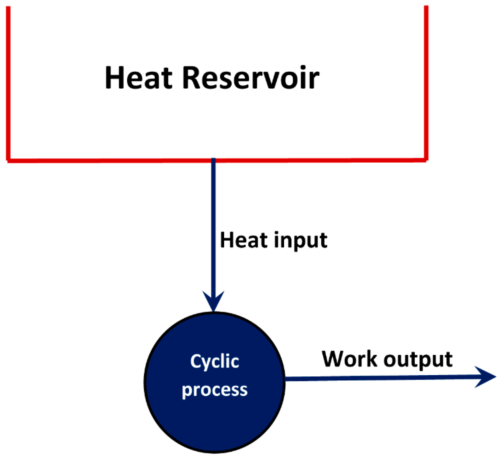
The Kelvin–Planck statement says that “It is impossible for a system operating in a cycle and connected to a single heat reservoir to produce a positive amount of work in the surroundings [3]”. According to the Kelvin–Planck statement, it is impossible to build a heat engine shown schematically in Figure 1 where heat absorbed from a heat reservoir is completely converted into work without altering the properties of the system. Mathematically, the Kelvin–Planck statement can be expressed as [4]:
where the system communicates thermally only with a single heat reservoir. The sign convention for work () used in this article is = positive, if it is produced by the system (flows out of the system to surroundings) and = negative, if it is absorbed by the system (flows into the system from surroundings). Thus, no cyclic process is possible where using a single heat reservoir. The equality in Equation (1) is valid for a reversible process and the inequality is valid for an irreversible process. For a reversible process, no work is produced or destroyed, that is, whereas work is destroyed when the process is irreversible, that is, (assuming that the system communicates thermally only with a single heat reservoir).
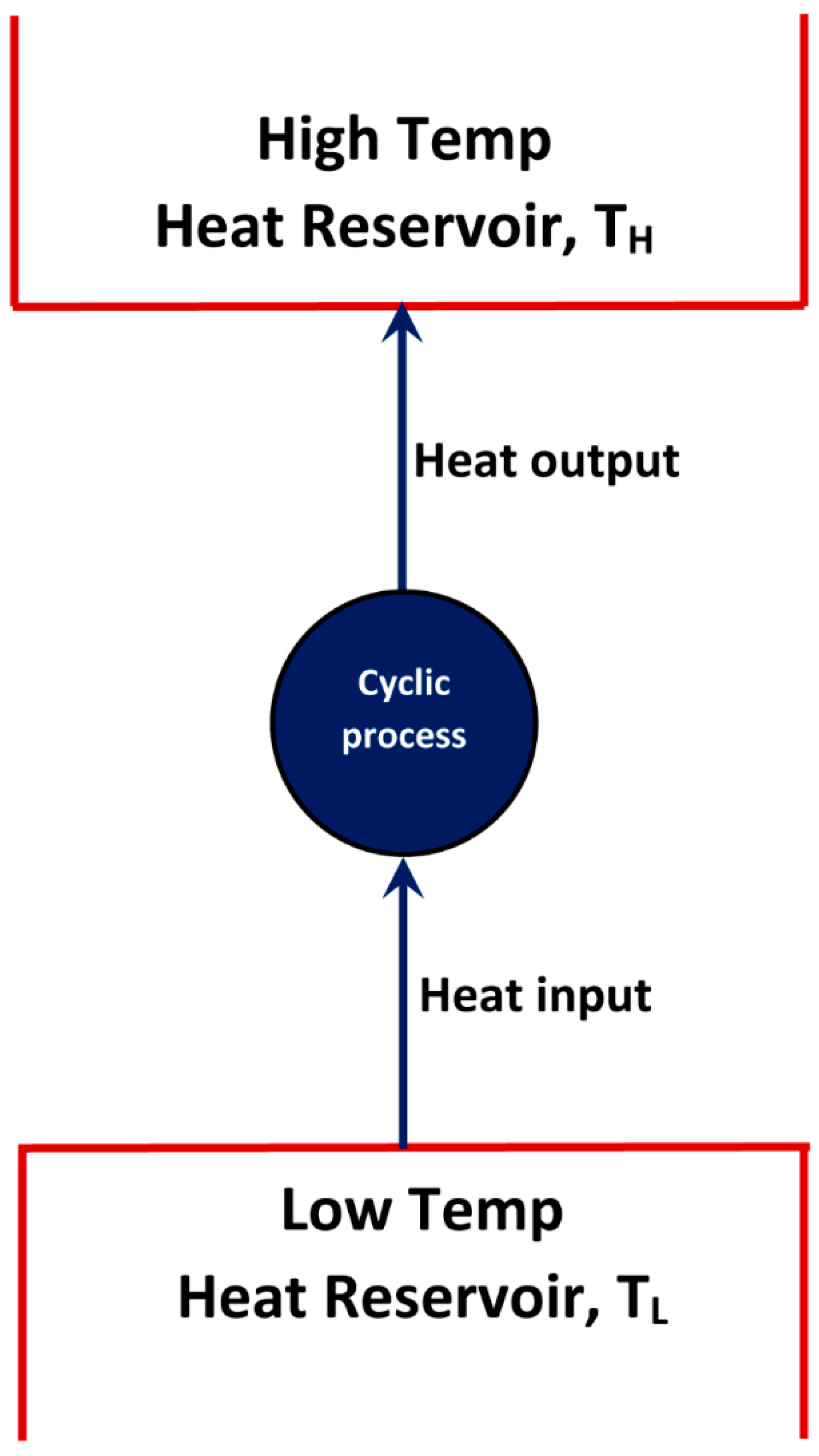
The Clausius statement of the second law [3] says that “It is impossible for a system operating in a cycle to have its sole effect the transfer of heat from a low temperature heat reservoir to a high temperature heat reservoir”. According to the Clausius statement, it is impossible to construct a device based on the scheme shown schematically in Figure 2 where the sole result of the process is the transfer of heat from a cooler body at low temperature () to a hotter body at high temperature (.
Another powerful statement of the second law of thermodynamics is that all irreversible (real) processes are accompanied by entropy generation in the universe [5], that is:
where is the total amount of entropy generated in the universe (system + surroundings), is the entropy change of the system and is the entropy change of the surroundings. The equality in Equation (2) is valid for a reversible process and the inequality is valid for an irreversible process. According to this statement of the second law, no process is possible for which .
Entropy is a measure of disorderliness of a system. According to the Boltzmann entropy equation, the entropy of a system can be expressed as [3]:
where is the number of possible configurations of the system and is the Boltzmann constant. The larger the number of possible configurations of the system, greater is the disorderliness of the system and higher is the entropy. Therefore, we can interpret the second law of thermodynamics in yet another way, that is, “Only those processes are possible processes which lead to an increase in the disorderliness of the universe”.
The scheme shown in Figure 1 is impossible as it decreases the disorder of the universe, that is, . Here but as the surroundings heat reservoir loses heat. For this scheme, Equation (2) gives:
where is the absolute temperature of the heat reservoir and is the heat transferred. As from the first law of thermodynamics, Equation (4) reduces to Equation (1), that is, when there is only one heat reservoir involved. Similarly, the scheme shown in Figure 2 is impossible as it decreases the disorder of the universe:
Note that as it loses heat whereas as it gains heat. However, due to different temperatures of the cold and hot bodies, .
Thus, the Kelvin–Planck and Clausius statements of the second law of thermodynamics are special cases of the statement of the second law expressed in the form of Equation (2).
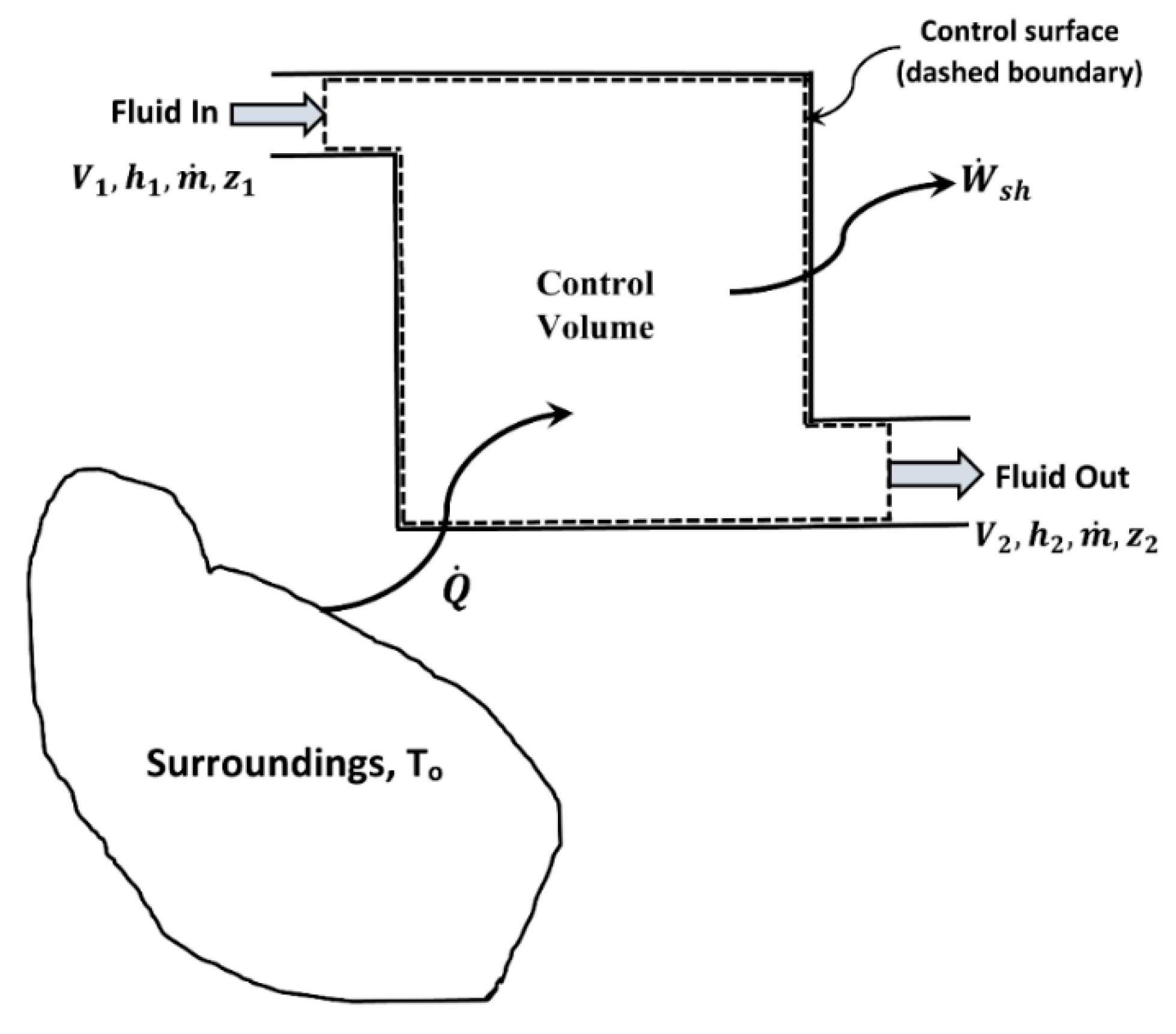
For a flow process (see Figure 3), the second law of thermodynamics can be written as [2]:
where is the rate of entropy generation, is the entropy per unit mass of fluid, is the fluid density, is unit outward normal to the control surface, is fluid velocity vector, is the control surface area, is time, is the volume of the control volume, is the rate of heat transfer to control volume from ith heat reservoir at an absolute temperature of , the subscripts and refer to control volume and surroundings, respectively. As noted earlier, the equality in Equation (6) is valid for a reversible (frictionless) process and the inequality is valid for an irreversible process. The surface integral is the net outward flow of entropy (associated with mass) across the entire control surface. The volume integral is the rate of accumulation of entropy within the entire control volume (assumed to be fixed and non-deforming). For a control volume with one inlet and one outlet, Equation (6), under steady state condition, reduces to:
where is the mass flow rate.
The quantification of entropy generation in real processes is important from a practical point of view as entropy generation is directly related to the efficiency of the process. Higher the rate of entropy generation in a process, lower is the thermodynamic efficiency of the process. According to the Gouy–Stodola theorem [6] of thermodynamics, the loss of power or work potential in a real process, due to irreversibilities in the process, is directly proportional to the total rate of entropy generation. Thus:
where is the rate of work lost (wasted) as a result of irreversibilities in the process.
As an example of a flow process, consider flow through a control volume shown in Figure 3. The first law of thermodynamics for open systems under steady state condition gives:
where is the specific enthalpy of fluid, is the fluid velocity, is the acceleration due to gravity, is the elevation, is the rate of heat transfer, and is the rate of shaft work. Neglecting kinetic and potential energy changes, Equation (9) simplifies to:
where is the heat transfer per unit mass of fluid. The second law, Equation (7), can be written as:
where is the absolute temperature of the heat reservoir (surroundings). For the flow process to be reversible:
where is the heat transfer per unit mass of fluid for a reversible process. From Equations (10) and (13):
The lost work, , is defined as:
From Equations (10), (14), and (15), we get:
Using Equation (11), Equation (16) can be re-written as:
Equation (17) is the Gouy–Stodola theorem [6] of thermodynamics. Thus, the rate of work lost due to irreversibilities is directly proportional to the rate of entropy generation. The thermodynamic efficiency of a flow process can be defined as:
In a reversible process, and . In any irreversible process, and . If no work is produced in the process, that is, actual is zero, then all the work potential is lost due to irreversibilities in the process and consequently, .
3. Flow through Unconsolidated and Consolidated Porous Media
Porous medium is a composite material in that it consists of two phases, namely pores (voids, free space pockets) and solid-phase. The pores may be occupied by a fluid (gas, oil, water, etc.). A large variety of natural and synthetic materials are porous in nature. Examples include: underground oil reservoirs, ceramics, solid foams, sand filters, wood, and packed beds of particles used widely in chemical engineering applications. The pores of a porous medium usually form a three-dimensional inter-connected network and, therefore, fluids can flow through the porous medium. If all pores of a porous medium are inter-connected, then the porosity ( of the porous medium is simply the fraction of the total volume of the medium that is occupied by the pores. Thus, the fraction of the total volume that is occupied by the solid phase is . When some pores are isolated or disconnected or have dead ends, then the effective porosity, defined as the ratio of connected void volume to total volume of the medium, is lower than the total porosity.
Porous media could be classified as consolidated or unconsolidated. In consolidated porous medium, the solid phase is basically a single piece of material or the grains of the solid phase are cemented or fused together to form a single piece of solid phase. In unconsolidated porous media, on the other hand, the grains or the particles of the solid phase are not cemented together and, therefore, the porous medium is a multi-particle system like a packed bed of individual (un-cemented, un-glued) particles. Flow of single-phase Newtonian fluids (gas, water, oil) through packed beds and consolidated porous media is important from a practical point of view.
3.1. Analysis of Flow through Packed Beds (Unconsolidated Porous Media)
3.1.1. Pressure-Loss in Flow through Packed Beds
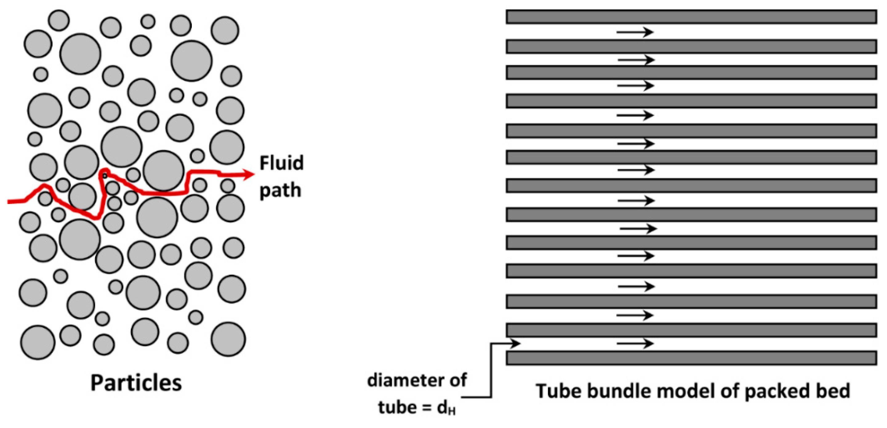
Consider flow of a Newtonian fluid through a horizontal cylindrical packed bed of particles with bed diameter and bed length . As flow through a packed bed is quite complex, a rigorous theoretical derivation of pressure drop-flow rate relationship is not possible. Only approximate models have been developed. In one approach, used widely to model flow through packed bed of particles, the packed bed is visualized as a bundle of identical capillary tubes [7,8,9]. In its simplest form, the capillary tube bundle model assumes that the capillary tubes are straight, cylindrical of constant cross-section (uniform radius), and parallel (all oriented in the same direction), as shown in Figure 4. The average velocity in any capillary tube is the same as that in the packed bed. The capillary diameter is equal to the hydraulic diameter of the bed, , defined as:
where is the void fraction or porosity, is the volume of a single particle, and is the surface area of a single particle. In writing the above expression for , it is assumed that all the particles are identical and that the wetted surface of the cylindrical container walls of the bed is negligible as compared with the total wetted surface area of the particles. For a bed of identical spherical particles, , where is the particle diameter. Thus, the hydraulic diameter becomes:
The superficial velocity of fluid () is defined is:
where is the volumetric flow rate of fluid and is the total cross-sectional area of the bed. Thus, is the velocity of fluid in the bed if no particles were present in the bed. The average velocity of fluid in the bed, also called interstitial velocity, is defined as:
where is the cross-sectional area of bed through which the fluid flows. The porosity of the bed is given as:
Therefore, the average or interstitial velocity of fluid in the bed is:
This expression of average velocity does not consider the tortuous path taken by fluid in the bed. Due to tortuosity of the bed, the actual average velocity of fluid in the bed is larger than that given by Equation (24). The tortuosity of a bed is defined as:
where is average length of the tortuous path taken by the fluid and is the straight length of the bed. To account for the tortuosity, the actual average velocity of the fluid in the bed can be expressed as follows:
In laminar flow of a Newtonian fluid through a cylindrical tube, the pressure gradient in the direction of flow is given as:
where is the fluid viscosity and is the tube diameter. Replacing with hydraulic diameter and the constant factor of 32 with , the pressure-gradient in a capillary tube model of the packed-bed model can be expressed as:
Note that flow in the bed is assumed to be laminar here. The constant is expected to be larger than 32, as the path of fluid in the bed is not straight. The fluid follows a tortuous path in the bed and consequently, the pressure drop over a certain straight length is expected to be more than that observed over the same length if the fluid path was non-tortuous. Therefore, the constant is taken as 32 where is the tortuosity. Upon substitution of the expressions for and , and taking C = 32 τ, Equation (28) gives:
Equation (29) assumes that the cross-section of the representative flow passage (capillary tube) in the porous medium is circular and constant. In reality the fluid moves through converging-diverging flow passages of non-uniform cross-sections. In converging-diverging flows, fluid experiences stretching or extensional deformation. The elongation or stretching of fluid elements results in additional dissipation of energy and pressure drop. Thus, this equation needs to be modified further as follows:
where is an empirical factor that takes into account the influence of non-constant cross-section of flow passage on pressure-gradient. The tortuosity τ is often taken to be for random packing of uniform spheres [9]. It is generally a function of the porosity of the porous medium [10]. For example, the following model, based on the Maxwell equation for electrical conductivity of composite, is often used to describe the relationship between tortuosity and porosity [10]:
When and , the following well-known Blake–Kozeny equation for laminar flow through randomly packed bed of uniform spheres is obtained [7]:
When and , the following Carman–Kozeny equation, another well-known equation for laminar flow through randomly packed bed of uniform spheres, is obtained [11]:
Both Blake–-Kozeny and Carman–Kozeny equations are popular in the literature although they use different values of the factor The observed difference in values is probably related to differences in particle-shape, surface roughness of particles, and porosity of bed. Note that these equations are restricted to only laminar flow through bed of nearly uniform spheres. The packed-bed Reynolds number , defined below, should be less than 10 for flow to be laminar in the bed.
For turbulent flow through packed beds , the following Burke–Plummer equation is often used [12]:
In the transition region, the following equation, obtained by superposition of Blake–Kozeny and Burke–Plummer equations, proposed by Ergun [13] is widely used:
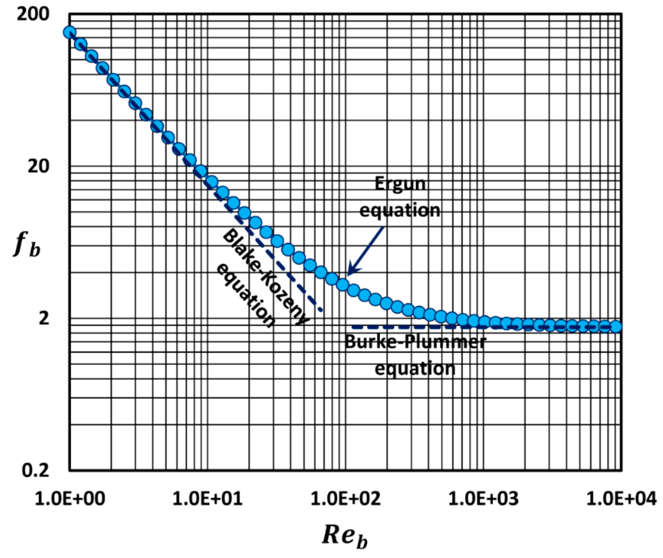
As the Ergun equation, Equation (36), is obtained by the superposition of laminar and turbulent expressions, it is valid over the full range of the packed-bed Reynolds number . The Ergun equation could also be re-cast in the following form [14]:
where is the packed-bed friction factor defined as:
The Ergun equation, Equation (36) or (37), is used extensively in the literature to describe pressure loss in packed beds. However, the following points should be kept in mind when using the Ergun equation: (a) it is applicable to unconsolidated beds of nearly uniform-size spherical particles with appreciable roughness. For smooth spheres, it tends to over-predict in the high range () [14,15,16]; (b) if the bed particles are non-uniform in sizes, the Sauter mean diameter of particles should be used in the application of the Ergun equation; (c) when particle shape deviates significantly from a sphere, the Ergun equation tends to under-predict [17]; and (d) wall effects can be important when . When wall effects are important, the experimental data show deviation from the predictions of the Ergun equation [18].
Figure 5 shows the prediction of the packed bed friction factor as a function of packed bed Reynolds number using the Ergun equation, Equation (37). In the limits of low and high , the Ergun equation predictions overlap with the predictions of the Blake–Kozeny equation (low ) and the Burke–Plummer equation (high ), as expected.
3.1.2. Entropy Generation in Flow through Packed Beds
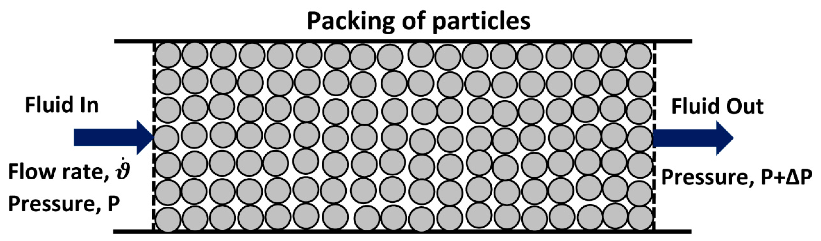
Consider steady flow of an incompressible fluid through a bed of particles (see Figure 6). We can apply the following macroscopic mechanical energy balance between the inlet and outlet of the bed [2]:
where is the rate of mechanical energy dissipation due to friction in fluid, is the potential energy change per unit mass of fluid, is the kinetic energy change per unit mass of fluid, and is the pressure change of the fluid. Neglecting potential and kinetic energy changes and taking , the mechanical energy balance gives:
The rate of mechanical energy dissipation per unit length of packed bed () can be expressed as:
From the second law of thermodynamics, Equation (11), we get:
Note that we are assuming flow to be adiabatic with negligible heat transfer. There is no entropy generation in the surroundings. All the entropy is generated within the fluid inside the packed bed and the rate of entropy generation is the net rate of increase in entropy of the flowing stream.
We can now relate entropy change of the fluid stream to pressure change. For pure substances, the relationship between entropy and other state variables is given as [5]:
where is the absolute temperature. From the first law of thermodynamics, Equation (9), the enthalpy change is zero in the absence of heat transfer and shaft work for steady flow in a horizontal bed. Consequently, Equation (43) reduces to:
Assuming incompressible flow and constant temperature, Equation (44) upon integration gives:
From Equations (42) and (45), it follows that:
The subscript “univ” has been removed from as is simply the rate of entropy generation within the fluid inside a packed bed. From Equations (41) and (46), we can also express the rate of entropy generation in a packed bed on a unit volume basis as:
where is the total cross-sectional area of the bed and is the rate of entropy generation per unit volume of the bed. From Equations (38) and (47), we get:
The packed bed friction factor for laminar flow ( is given as:
Consequently, Equation (48) reduces to:
Thus, entropy generation rate per unit volume of bed in steady laminar flow of a Newtonian fluid is directly proportional to the fluid viscosity and to the square of the superficial fluid velocity in the bed. The entropy generation rate also depends on the particle diameter, the bed porosity , and the temperature.
The packed bed friction factor in turbulent flow () is given as [7,8,9]:
Consequently, Equation (48) reduces to:
Thus, entropy generation rate per unit volume of bed in steady turbulent flow of a Newtonian fluid is independent of the fluid viscosity and is directly proportional to the cube of the superficial fluid velocity in the bed. The entropy generation rate also depends on the fluid density, the particle diameter, the bed porosity , and the temperature.
To cover the full range of packed bed Reynolds number , we substitute the Ergun equation, Equation (37), into Equation (48) to obtain the following equation valid over the full range of packed bed Reynolds number :
Note that Equation (53) is simply the superposition of Equations (50) and (52).
3.2. Analysis of Flow through Consolidated Porous Media
3.2.1. Pressure-Loss in Flow through Consolidated Porous Media
Laminar flow in consolidated porous media (see Figure 7) is usually described by Darcy’s law given as follows [19]:
where is the permeability of the porous medium. Permeability is a measure of the ability of porous medium to conduct fluid. Higher means lower resistance to flow and consequently, larger flow rate for the same pressure gradient. has the dimensions of (length)2. It is usually expressed in darcies. For example, 1 darcy = 1 (cm/s). centipoise/(atm/cm) = 9.87 × 10⁻¹³ m2.
Darcy’s law is equally applicable to unconsolidated porous medium such as packed bed of free (un-cemented/un-fused) particles. Thus, the Blake–Kozeny equation or the Carman–Kozeny equation are special cases of the Darcy law. Upon comparison of the Darcy law with Blake–Kozeny/Carman–Kozeny equations, the permeability of a packed bed of uniform size spherical particles can be expressed as follows:
Equation (55) gives permeability based on the Blake–Kozeny equation whereas Equation (56) gives permeability based on the Carman–Kozeny equation.
Darcy’s law is restricted to flows where viscous forces dominate over the inertial forces. At high flow rates, the flow in the porous medium becomes turbulent and Darcy’s law is no longer valid. The pressure-gradient in the turbulent regime is much higher compared with that in the laminar regime at the same superficial velocity . In order to extend the Darcy law to turbulent regime, Forchheimer [19] modified the Darcy law by adding a quadratic term as follows:
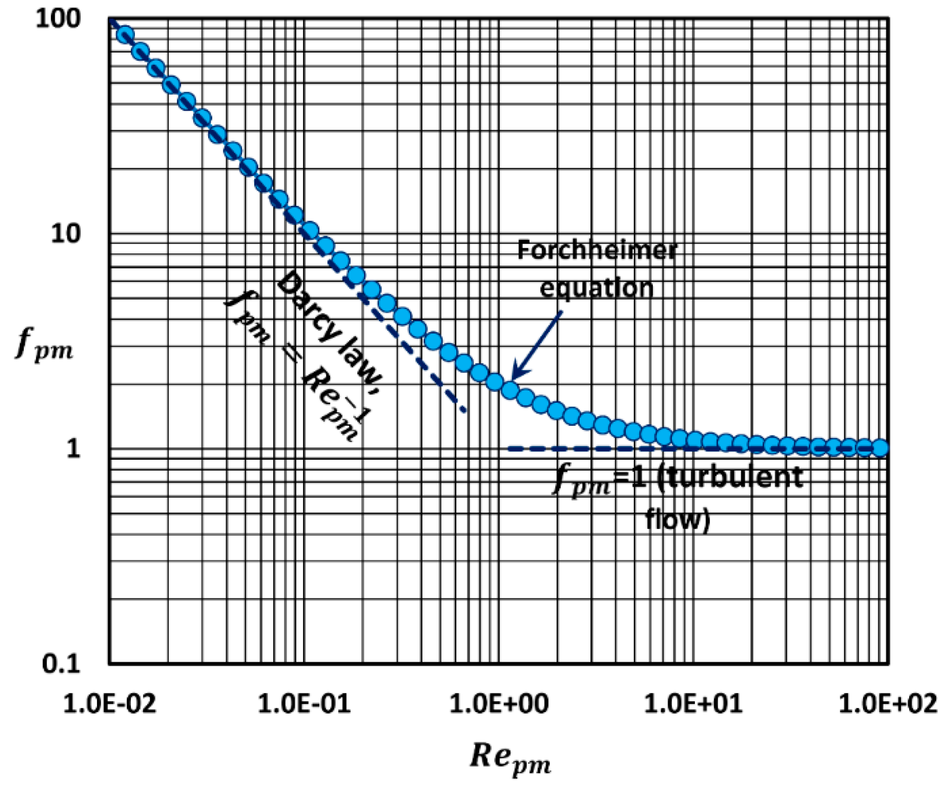
where the first term on the right side of the equation reflects the viscous effects and the second term reflects the inertial effects. is called the non-Darcy flow coefficient with a dimension of 1/length. This equation could be re-written in dimensionless form as:
where is the friction factor for flow in consolidated porous medium and is the porous-medium Reynolds number, also referred to as Forchheimer number, defined as:
At low Reynolds number (), the first term on the right side of the dimensionless Forchheimer equation, Equation (58), can be neglected and it reduces to Darcy’s law. At high Reynolds number (), the second term on the right side of the dimensionless Forchheimer equation, Equation (58), can be neglected and it reduces to . Figure 8 shows the prediction of as a function of using the Forchheimer equation, Equation (58).
In order to apply the Forchheimer equation, the value of non-Darcy flow coefficient is needed. It can be determined experimentally. The experimental procedure to determine β involves two steps: In the first step, the permeability of the porous sample is determined from Darcy’s law by restricting the experiments to low flow rates, and in the second step, the experiments are conducted at high flow rates and is evaluated directly from the Forchheimer equation from the knowledge of pressure drop versus flow rate. The non-Darcy flow coefficient decreases with the increase in the permeability of the porous medium [20].
The Forchheimer equation is equally applicable to unconsolidated porous medium such as a packed bed of particles. Ergun equation is a special case of the Forchheimer equation. The Forchheimer equation, Equation (57) reduces to the Ergun equation, Equation (36), when permeability and non-Darcy flow coefficient are replaced by the following expressions:
The relationships between and , and and are as follows:
3.2.2. Entropy Generation in Flow through Consolidated Porous Media
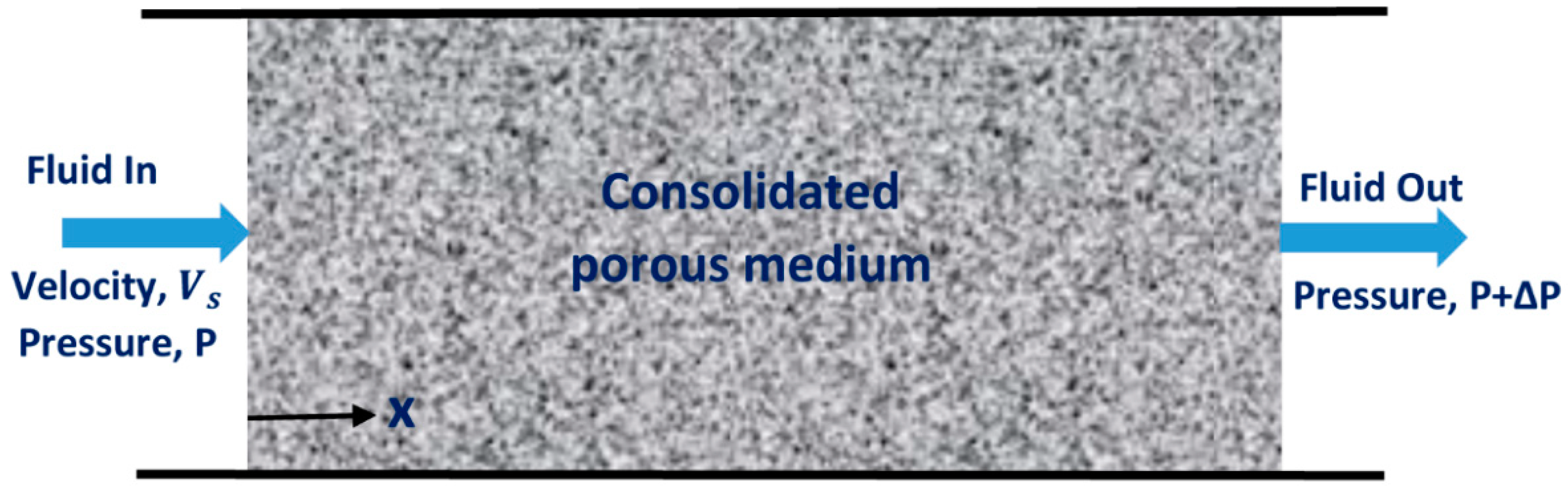
Consider one-dimensional flow of an incompressible Newtonian fluid in consolidated porous medium, as shown in Figure 9. The rate of entropy generation in consolidated porous medium per unit volume is given by Equation (47), re-written as:
The porous medium friction factor for laminar flow ( is given as:
Consequently, Equation (63) reduces to:
Thus, entropy generation rate per unit volume of the porous medium in steady laminar flow of a Newtonian fluid is directly proportional to the fluid viscosity, inversely proportional to the porous medium permeability, and directly proportional to the square of the superficial fluid velocity in the medium. The entropy generation rate also depends on the temperature.
The porous medium friction factor in turbulent flow () is given as:
Consequently, Equation (63) reduces to:
Thus, entropy generation rate per unit volume of the porous medium in steady turbulent flow of a Newtonian fluid is independent of the fluid viscosity and is directly proportional to the cube of the superficial fluid velocity in the bed. The entropy generation rate also depends on the fluid density, the non-Darcy flow coefficient , and the temperature.
To cover the full range of porous medium Reynolds number , we substitute the Forchheimer equation, Equation (58), into Equation (63) to obtain the following equation valid over the full range of porous medium Reynolds number :
Equation (68) is simply the superposition of Equations (65) and (67).
4. Simulation Results and Discussion
4.1. Entropy Generation in Flow through Packed Beds
4.1.1. Laminar Flow
The entropy generation rate in laminar flow through packed beds, per unit volume of the bed, as a function of superficial bed velocity is shown in Figure 10 for the following conditions: = 298.15 K, = 1 mm, = 18.5 µPa·s, and = 1.184 kg/m3. Equation (50) is used to generate the plots. For a given value of the bed porosity , the entropy generation rate increases with the increase in the superficial velocity of the fluid in the bed.
The increase in with the increase in is larger if the bed porosity is small. Additionally, the entropy generation rate falls sharply with the increase in the bed porosity. These results are as expected. With the increase in the fluid velocity, the rate of mechanical energy dissipation into frictional heat increases due to increases in viscous stresses and velocity gradients in the fluid. Consequently, there occurs an increase in the rate of entropy generation. When the bed porosity is increased, the bed structure becomes more open to fluid flow resulting in a decrease in the resistance to fluid motion and mechanical energy dissipation and, hence, a decrease in the rate of entropy generation.
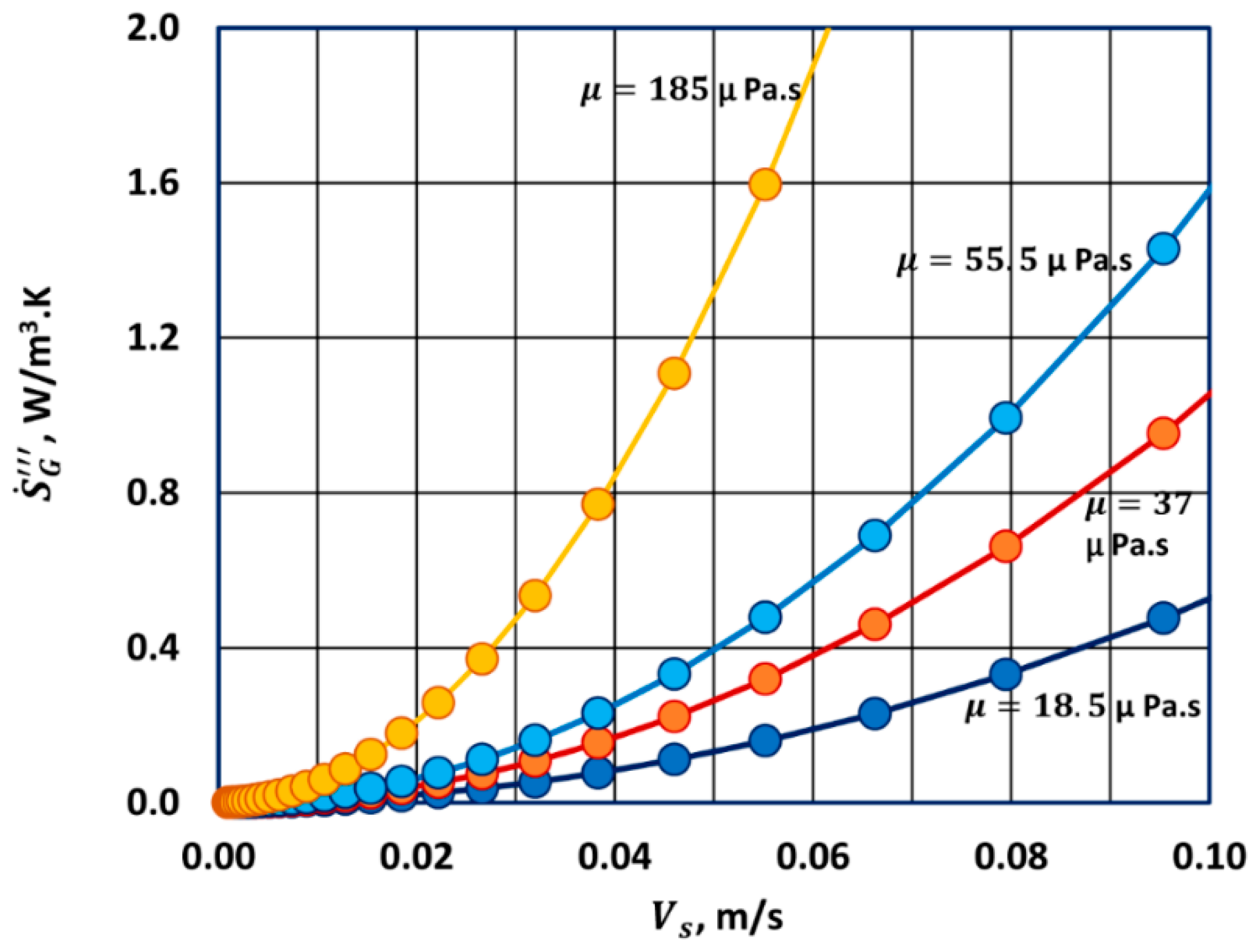
Figure 11 shows the effect of fluid viscosity on the rate of entropy generation in laminar flow. The plots are generated using Equation (50). With the increase in fluid viscosity, the resistance to fluid motion increases due to an increase in the viscous stresses. With the increase in viscous stresses, the rate of mechanical energy dissipation into frictional heat (internal energy) increases. The conversion of highly ordered mechanical energy into disorderly internal energy is reflected in an increase in the rate of entropy generation.
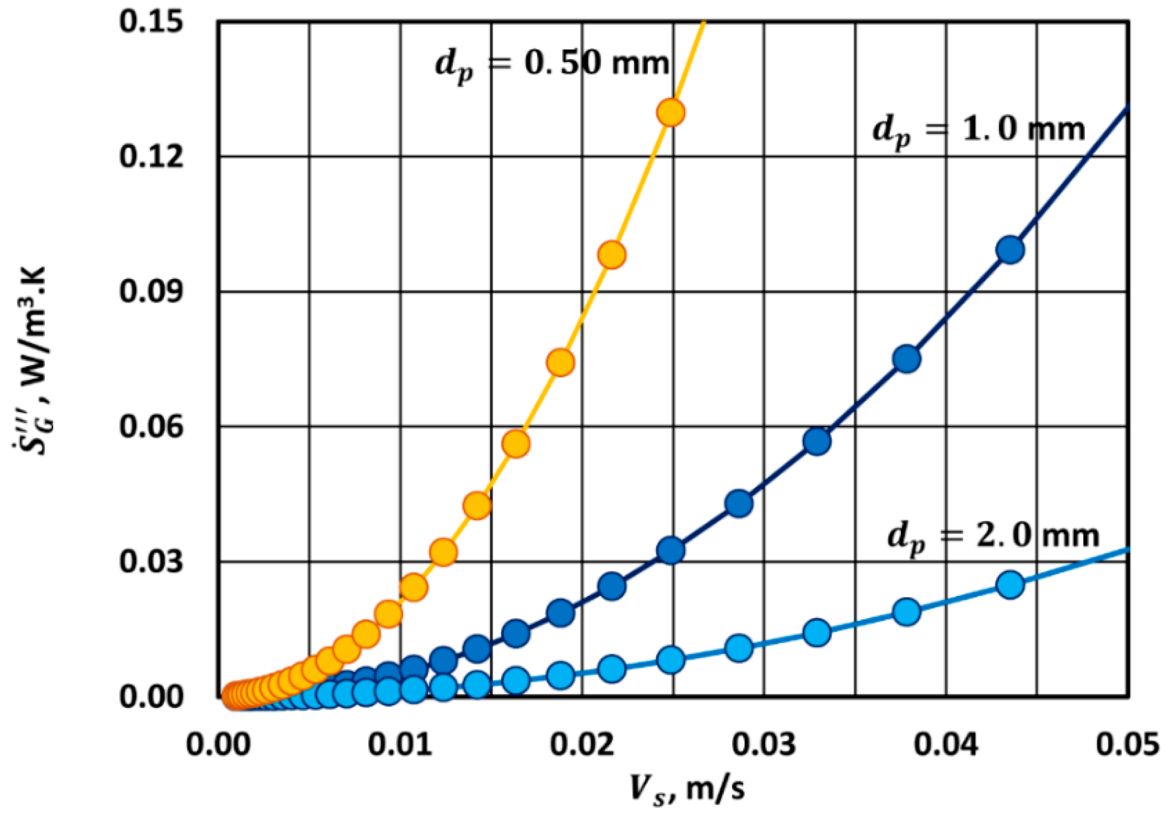
The effect of particle diameter on the rate of entropy generation in laminar flow through packed beds is shown in Figure 12. A sharp reduction in the rate of entropy generation occurs with the increase in the particle diameter. With the increase in the particle diameter, the number density of particles is decreased for the same bed porosity . It can be readily shown that the number of particles per unit volume of bed and the fluid-solids contact area per unit volume of bed are:
Equation (69) assumes that the particles are uniform spheres of diameter . The decrease in the number density of particles with the increase in particle diameter results in a decrease in contact area between the fluid and solids resulting in a decrease in the resistance to fluid motion. Consequently the rate of mechanical energy dissipation into internal energy and hence the rate of entropy generation decrease with the increase in particle diameter.
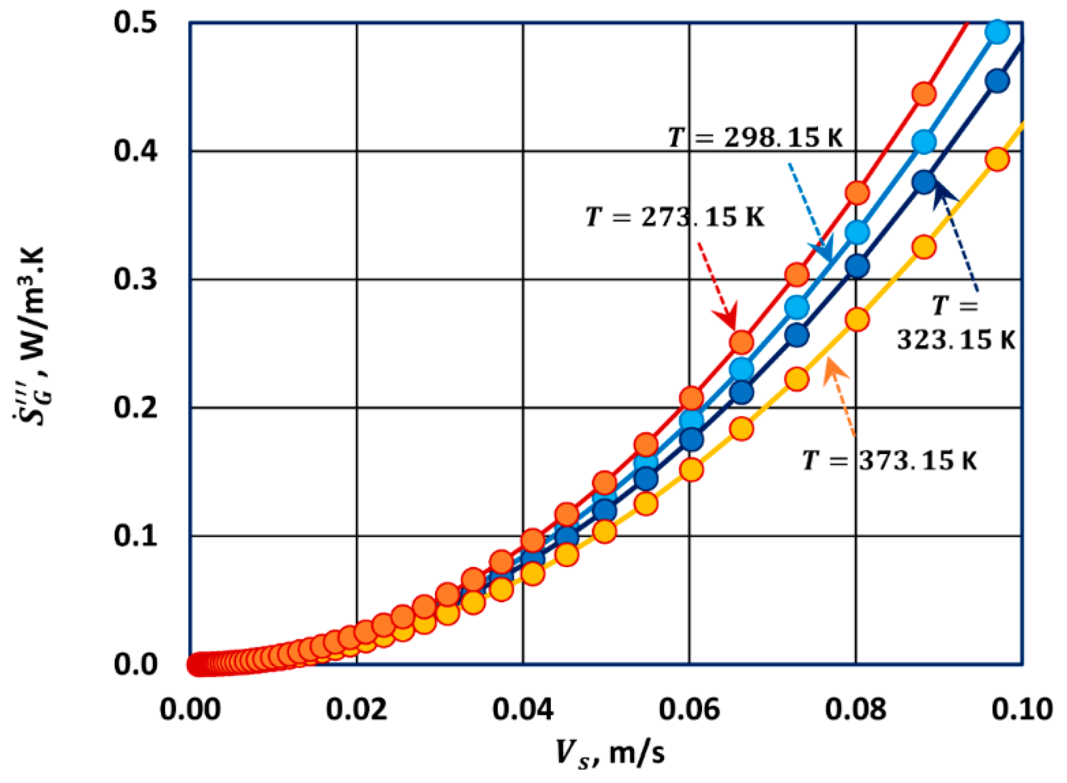
Figure 13 shows the effect of temperature on the rate of entropy generation in laminar flow through packed beds. The rate of entropy generation decreases with the increase in temperature keeping other factors (fluid properties, bed characteristics) constant. At a given fluid velocity , the rate of mechanical energy dissipation into internal energy is the same at different temperatures as the fluid properties are kept constant. Then why does the rate of entropy generation decrease with the increase in temperature? It so happens that the increase in entropy with the increase in internal energy is sensitive to temperature. For incompressible materials, the rate of change of entropy with respect to internal energy, that is, the derivative is given as:
Higher the temperature, smaller is the increase in entropy for the same increase in internal energy.
4.1.2. Turbulent Flow
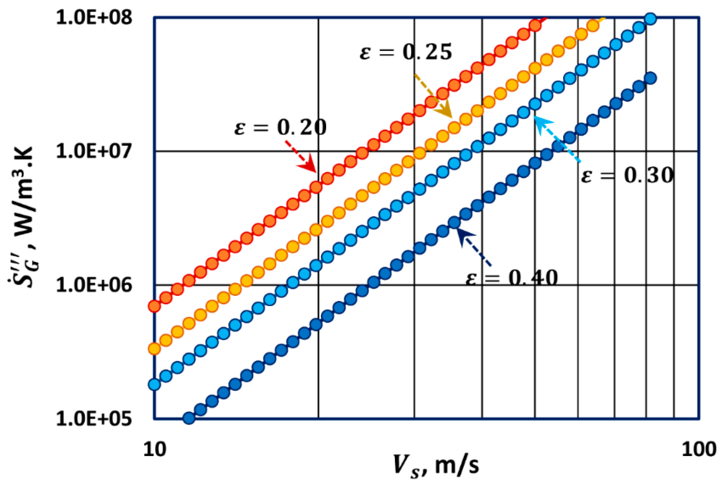
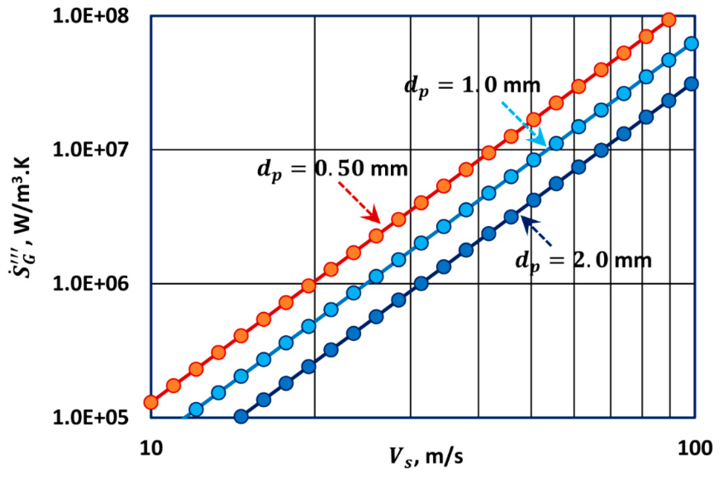
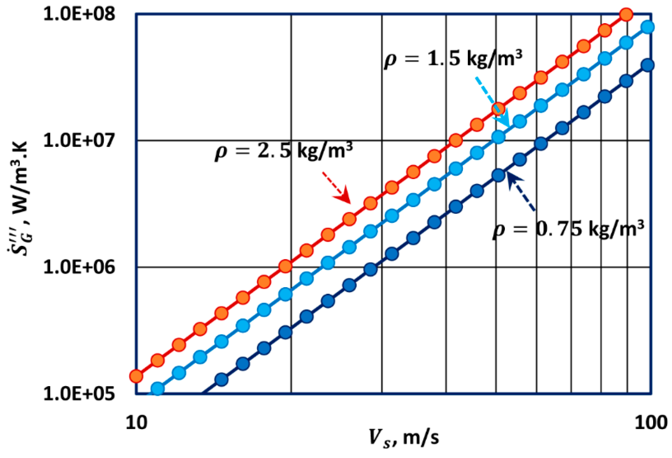
Figure 14, Figure 15 and Figure 16 show the entropy generation rates for turbulent flow through packed beds under different conditions. Due to broad ranges of entropy generation rates and superficial fluid velocities, the plots are drawn using log-log scale. The plots on log-log scale are linear with a slope of 3 as expected from Equation (52). With the increases in bed porosity and particle diameter, the entropy generation rates decrease due to a decrease in the resistance to fluid motion and mechanical energy dissipation. There is no dependence of entropy generation on fluid viscosity in turbulent flow. However, fluid density now plays a role. With the increase in fluid density, the rate of entropy generation in turbulent flow increases due to an increase in the resistance to fluid motion and mechanical energy dissipation caused by inertial effects.
Figure 17 shows the entropy generation rate in a packed bed over a broad range of fluid superficial velocity covering the full range of packed bed Reynolds number. The plot is generated from Equation (53) under the following conditions: = 298.15 K, = 0.40, = 1 mm, = 18.5 µPa·s, and = 1.184 kg/m3. The predictions of Equation (53) overlap with the two asymptotes, Equation (50) for low velocities and Equation (52) for high velocities.
4.2. Entropy Generation in Flow through Consolidated Porous Media
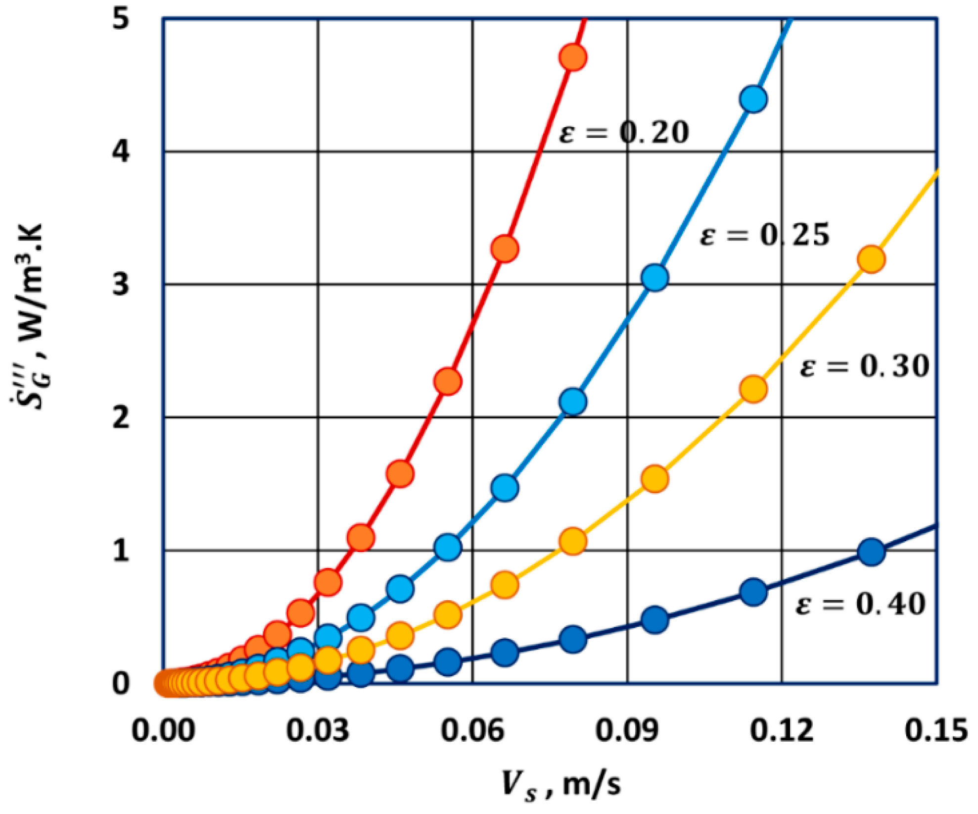
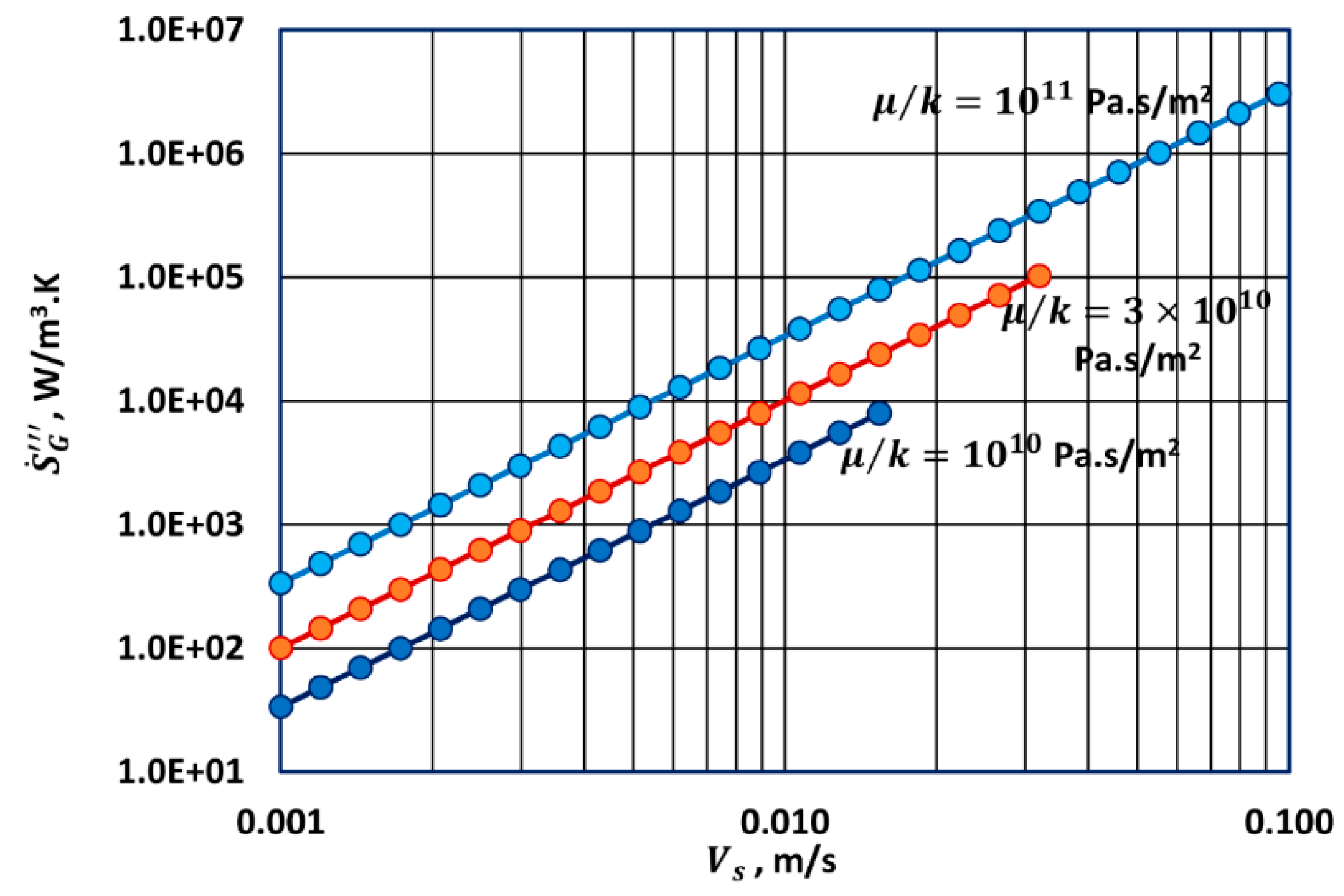
The entropy generation rate in laminar flow through consolidated porous medium is given by Equation (65). The key factor affecting the vs. behavior is the ratio of fluid viscosity to permeability, . Figure 18 shows the plots of vs. for different values of . The plots on a log-log scale are linear with slopes of 2. With the increase in ratio, the entropy generation rate increases at any given superficial velocity . When the fluid viscosity is increased (keeping the same), the entropy generation rate increases due to an increase in mechanical energy dissipation caused by viscous stresses. When the permeability of the porous medium is decreased (keeping the same), the porous medium becomes less permeable to fluid flow resulting in larger resistance to fluid motion and hence larger rates of mechanical energy dissipation and entropy generation. Note that is typically in the range of 10−15 to 10−12 m2 for porous sandstones [20].
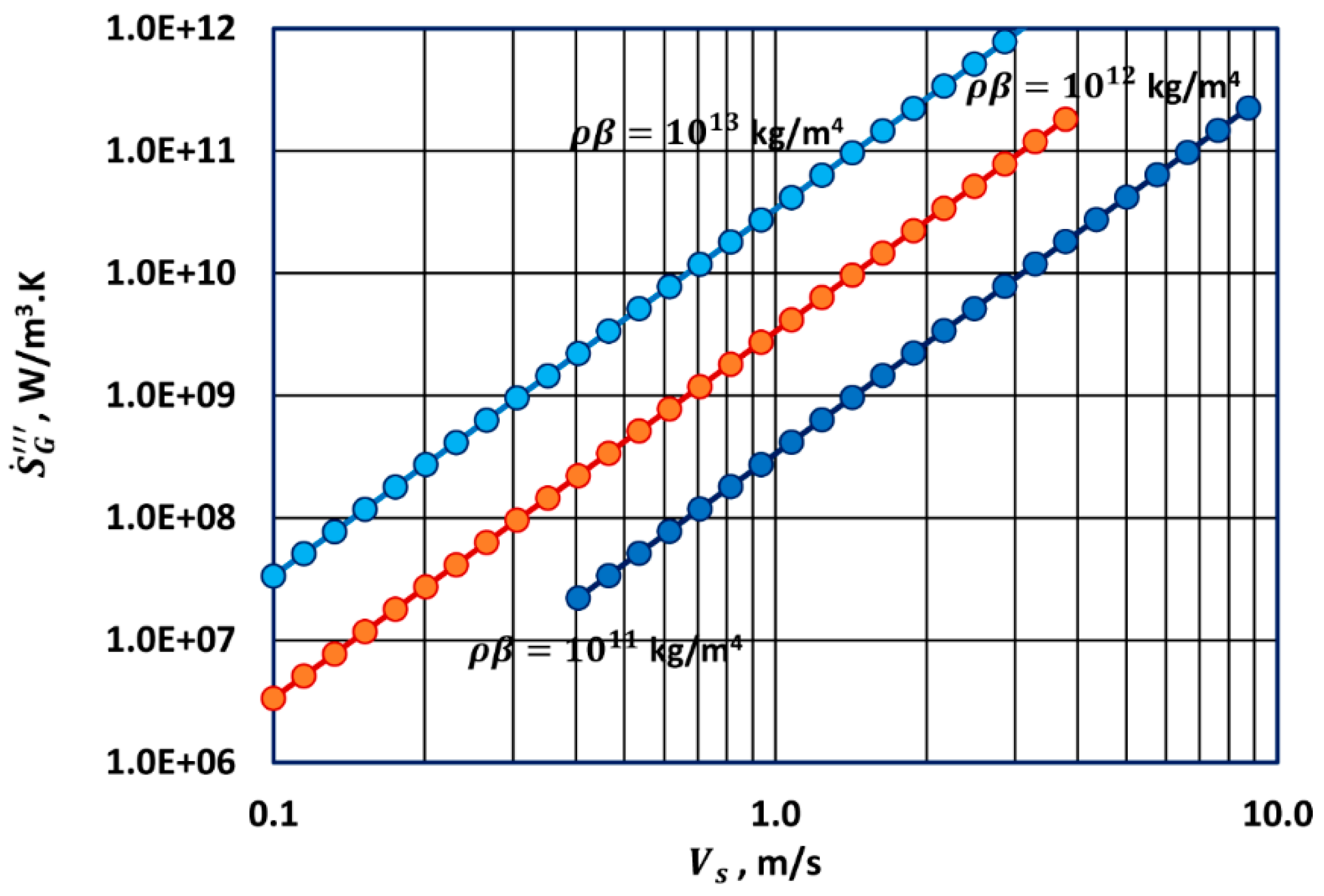
In turbulent flow through consolidated porous medium, the key factor governing the vs. behavior is where is the non-Darcy flow coefficient. With the increase in , the entropy generation rate increases at any given , as shown in Figure 19. Note that the non-Darcy flow coefficient is inversely related to the porous medium permeability [20]. For sandstones, is typically in the range of 108 to 1012 m−1. With the increase in , the porous medium becomes less permeable to fluid flow resulting in an increase in the resistance to fluid motion. Consequently, the rates of mechanical energy dissipation and entropy generation increase with the increase in . The fluid density has a similar effect on entropy generation rate in the turbulent regime.
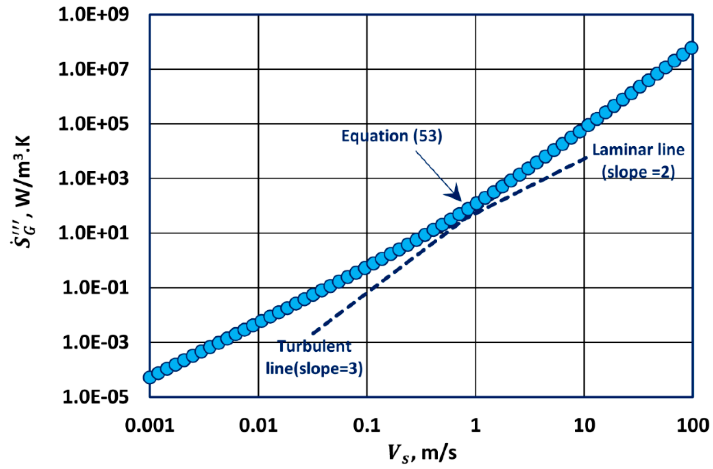
Figure 20 shows the entropy generation rate in a consolidated porous medium over a broad range of fluid superficial velocity (10−4 ≤ ≤ 10 m/s) covering laminar, transition, and turbulent flow regimes. The plot is generated from Equation (68) under the following conditions: = 298.15 K, = 1 mPa·s, = 1000 kg/m3, = 10−12 m2, = 108 m−1. The predictions of Equation (68) overlap with the limiting low asymptote (Equation (65)) at low superficial velocities and with the high asymptote (Equation (67)) at high superficial velocities.
5. Conclusions
In conclusion, a novel approach is described to teach the second law of thermodynamics via the analysis of flow through packed beds and consolidated porous media. The second law of thermodynamics and the relevant background in fluid mechanics are reviewed briefly. The link between entropy generation and mechanical energy dissipation in flow through packed beds and consolidated porous media is established in terms of the directly measureable pressure loss. Equations are developed to predict the entropy generation rates in a porous medium in terms of the flow variables, fluid properties, and structural properties of the medium. Simulation results dealing with entropy generation in a porous medium are presented and discussed. The proposed approach can be implemented at an undergraduate level either as an experimental exercise dealing with pressure loss measurements in flow through a porous medium such as a packed bed or as a simulation exercise. The material presented in the article is suited for third year engineering students after they have completed introductory courses in fluid mechanics and thermodynamics.
Funding
This research received no external funding.
Conflicts of Interest
The author declares no conflict of interest.
References
- Pal, R. Conceptual issues related to reversibility and reversible work in closed and open flow systems. Educ. Chem. Eng. 2017, 19, 29–37. [Google Scholar] [CrossRef]
- Pal, R. Teaching fluid mechanics and thermodynamics simultaneously through pipeline flow experiments. Fluids 2019, 4, 103. [Google Scholar] [CrossRef]
- Castellan, G.W. Physical Chemistry, 3rd ed.; Benjamin/Cummings Pub. Co: Menlo Park, CA, USA, 1983. [Google Scholar]
- Bejan, A.; Tsatsaronis, G.; Moran, M. Thermal Design and Optimization; Wiley: New York, NY, USA, 1996. [Google Scholar]
- Smith, J.M.; Van Ness, H.C.; Abbott, M.M. Introduction to Chemical Engineering Thermodynamics, 7th ed.; McGraw-Hill: New York, NY, USA, 2005. [Google Scholar]
- Pal, R. On the Gouy−Stodola theorem of thermodynamics for open systems. Int. J. Mech. Eng. Educ. 2017, 45, 194–206. [Google Scholar] [CrossRef]
- Bird, R.B.; Stewart, W.E.; Lightfoot, E.N. Transport Phenomena, 2nd ed.; Wiley: New York, NY, USA, 2007. [Google Scholar]
- Wilkes, J.O. Fluid Mechanics for Chemical Engineers, 3rd ed.; Prentice Hall: Boston, MA, USA, 2018. [Google Scholar]
- Chhabra, R.P.; Richardson, J.F. Non-Newtonian Flow in Process Industries; Butterworth Heinemann: Oxford, UK, 1999. [Google Scholar]
- Barrande, M.; Bouchet, R.; Denoyel, R. Tortuosity of porous particles. Anal. Chem. 2007, 79, 9115–9121. [Google Scholar] [CrossRef] [PubMed]
- Kruczek, B. Carman−Kozeny equation. In Encyclopedia of Membranes; Droli, E., Giorno, L., Eds.; Springer: Berlin, Germany, 2014. [Google Scholar]
- Burke, S.P.; Plummer, W.B. Gas flow through packed columns. Ind. Eng. Chem. 1928, 20, 1196–1200. [Google Scholar] [CrossRef]
- Ergun, S. Flow through packed columns. Chem. Eng. Prog. 1952, 48, 89–94. [Google Scholar]
- Allen, K.G.; Von Backstrom, T.W.; Kroger, D.G. Packed bed pressure drop dependence on particle shape, size distribution, packing arrangement and roughness. Powder Technol. 2013, 246, 590–600. [Google Scholar] [CrossRef]
- Tallmadge, J.A. Packed bed pressure drop—An extension to higher Reynolds numbers. AIChE J. 1970, 16, 1092–1093. [Google Scholar] [CrossRef]
- Wentz, C.A.; Thodos, G. Pressure drops in the flow of gases through packed and distended beds of spherical particles. AIChE J. 1963, 9, 81–84. [Google Scholar] [CrossRef]
- Mayerhofer, M.; Govaerts, J.; Parmentier, N.; Jeanmart, H.; Helsen, L. Experimental investigation of pressure drop in packed beds of irregular shaped wood particles. Powder Technol. 2011, 205, 30–35. [Google Scholar] [CrossRef]
- Pesic, R.; Kaluderovic-Radoicic, T.K.; Boskovic-Vragolovic, N.; Arsenijevic, Z.; Grbavcic, Z. Pressure drop in packed beds of spherical particles at ambient and elevated air temperatures. Chem. Ind. Chem. Eng. 2015, 21, 419–427. [Google Scholar] [CrossRef]
- De Schampheleire, S.; De Kerpel, K.; Ameel, B.; De Jaeger, P.; Bagci, O.; De Paepe, M. A discussion on the interpretation of the Darcy equation in case of open-cell metal foam based on numerical simulations. Materials 2016, 9, 409. [Google Scholar] [CrossRef] [PubMed]
- Choi, C.S.; Song, J.J. Estimation of the Non-Darcy coefficient using supercritical CO2 and various sandstones. JCR Solid Earth 2019, 124, 442–455. [Google Scholar]
Figure 1.
Impossible heat engine.

Figure 2.
Impossible scheme.

Figure 3.
Typical flow process.

Figure 4.
Path taken by fluid in a bed of particles and tube bundle model of packed bed.

Figure 5.
Prediction of packed bed friction factor as a function of packed bed Reynolds number. The data points are generated using the Ergun equation (Equation (37)).
Figure 5.
Prediction of packed bed friction factor as a function of packed bed Reynolds number. The data points are generated using the Ergun equation (Equation (37)).

Figure 6.
Flow through a packed bed

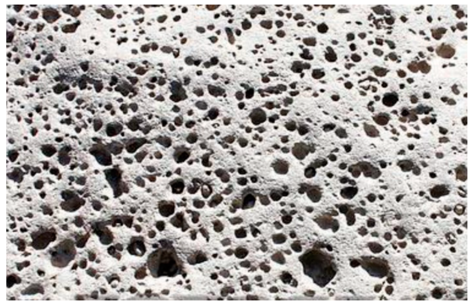
Figure 7.
Consolidated porous medium (adapted from www.fotosearch.com.au).
Figure 7.
Consolidated porous medium (adapted from www.fotosearch.com.au).

Figure 8.
Prediction of porous medium friction factor as a function of porous medium Reynolds number. The data points are generated using the Forchheimer equation (Equation (58)).
Figure 8.
Prediction of porous medium friction factor as a function of porous medium Reynolds number. The data points are generated using the Forchheimer equation (Equation (58)).

Figure 9.
One-dimensional flow in consolidated porous medium.

Figure 10.
Effect of bed porosity on the rate of entropy generation per unit volume of the packed bed in laminar flow ( = 298.15 K, = 1 mm, = 18.5 µPa·s, = 1.184 kg/m3). The data points are generated using Equation (50).
Figure 10.
Effect of bed porosity on the rate of entropy generation per unit volume of the packed bed in laminar flow ( = 298.15 K, = 1 mm, = 18.5 µPa·s, = 1.184 kg/m3). The data points are generated using Equation (50).

Figure 11.
Effect of fluid viscosity on the rate of entropy generation per unit volume of the packed bed in laminar flow ( = 298.15 K, = 1 mm, = 0.40, kg/m3). The data points are generated using Equation (50).
Figure 11.
Effect of fluid viscosity on the rate of entropy generation per unit volume of the packed bed in laminar flow ( = 298.15 K, = 1 mm, = 0.40, kg/m3). The data points are generated using Equation (50).

Figure 12.
Effect of particle diameter on the rate of entropy generation per unit volume of the packed bed in laminar flow ( = 298.15 K, = 0.40, = 18.5 µPa·s, kg/m3). The data points are generated using Equation (50).
Figure 12.
Effect of particle diameter on the rate of entropy generation per unit volume of the packed bed in laminar flow ( = 298.15 K, = 0.40, = 18.5 µPa·s, kg/m3). The data points are generated using Equation (50).

Figure 13.
Effect of temperature on the rate of entropy generation per unit volume of the packed bed in laminar flow ( = 0.40, = 1 mm, = 18.5 µPa·s, kg/m3). The data points are generated using Equation (50).
Figure 13.
Effect of temperature on the rate of entropy generation per unit volume of the packed bed in laminar flow ( = 0.40, = 1 mm, = 18.5 µPa·s, kg/m3). The data points are generated using Equation (50).

Figure 14.
Effect of bed porosity on the rate of entropy generation per unit volume of the packed bed in turbulent flow ( = 298.15 K, = 1 mm, = 18.5 µPa·s, kg/m3). The data points are generated using Equation (52).
Figure 14.
Effect of bed porosity on the rate of entropy generation per unit volume of the packed bed in turbulent flow ( = 298.15 K, = 1 mm, = 18.5 µPa·s, kg/m3). The data points are generated using Equation (52).

Figure 15.
Effect of particle diameter on the rate of entropy generation per unit volume of the packed bed in turbulent flow ( = 298.15 K, = 0.40, = 18.5 µPa·s, kg/m3). The data points are generated using Equation (52).
Figure 15.
Effect of particle diameter on the rate of entropy generation per unit volume of the packed bed in turbulent flow ( = 298.15 K, = 0.40, = 18.5 µPa·s, kg/m3). The data points are generated using Equation (52).

Figure 16.
Effect of fluid density on the rate of entropy generation per unit volume of the packed bed in turbulent flow ( = 298.15 K, = 0.40, = 1 mm, = 18.5 µPa·s). The data points are generated using Equation (52).
Figure 16.
Effect of fluid density on the rate of entropy generation per unit volume of the packed bed in turbulent flow ( = 298.15 K, = 0.40, = 1 mm, = 18.5 µPa·s). The data points are generated using Equation (52).

Figure 17.
Prediction of for packed beds over a broad range of fluid superficial velocity under the conditions: = 298.15 K, = 0.40, = 1 mm, = 18.5 µPa·s, and = 1.184 kg/m3. The data points are generated using Equation (53).
Figure 17.
Prediction of for packed beds over a broad range of fluid superficial velocity under the conditions: = 298.15 K, = 0.40, = 1 mm, = 18.5 µPa·s, and = 1.184 kg/m3. The data points are generated using Equation (53).

Figure 18.
Effect of viscosity to permeability ratio () on the rate of entropy generation per unit volume of consolidated porous medium in laminar flow ( = 298.15 K, = 108 m−1, = 103 kg/m3). The data points are generated using Equation (65).
Figure 18.
Effect of viscosity to permeability ratio () on the rate of entropy generation per unit volume of consolidated porous medium in laminar flow ( = 298.15 K, = 108 m−1, = 103 kg/m3). The data points are generated using Equation (65).

Figure 19.
Effect of on the rate of entropy generation per unit volume of consolidated porous medium in turbulent regime ( = 298.15 K, = 10 mPa·s, = 10−12 m2). The data points are generated using Equation (67).
Figure 19.
Effect of on the rate of entropy generation per unit volume of consolidated porous medium in turbulent regime ( = 298.15 K, = 10 mPa·s, = 10−12 m2). The data points are generated using Equation (67).

Figure 20.
Prediction of for consolidated porous medium over a broad range of fluid superficial velocity under the conditions: = 298.15 K, = 1mPa·s, = 1000 kg/m3, = 10−12 m2, = 108 m−1. The data points are generated using Equation (68).
Figure 20.
Prediction of for consolidated porous medium over a broad range of fluid superficial velocity under the conditions: = 298.15 K, = 1mPa·s, = 1000 kg/m3, = 10−12 m2, = 108 m−1. The data points are generated using Equation (68).

© 2019 by the author. Licensee MDPI, Basel, Switzerland. This article is an open access article distributed under the terms and conditions of the Creative Commons Attribution (CC BY) license (http://creativecommons.org/licenses/by/4.0/).
Share and Cite
MDPI and ACS Style
Pal, R. Teach Second Law of Thermodynamics via Analysis of Flow through Packed Beds and Consolidated Porous Media. Fluids 2019, 4, 116. https://0-doi-org.brum.beds.ac.uk/10.3390/fluids4030116
AMA Style
Pal R. Teach Second Law of Thermodynamics via Analysis of Flow through Packed Beds and Consolidated Porous Media. Fluids. 2019; 4(3):116. https://0-doi-org.brum.beds.ac.uk/10.3390/fluids4030116
Chicago/Turabian StylePal, Rajinder. 2019. "Teach Second Law of Thermodynamics via Analysis of Flow through Packed Beds and Consolidated Porous Media" Fluids 4, no. 3: 116. https://0-doi-org.brum.beds.ac.uk/10.3390/fluids4030116