Understanding Fluid Dynamics from Langevin and Fokker–Planck Equations


1
Department of Mathematics, University of South Carolina, Columbia, SC 29208, USA
2
Department of Mechanical and Aerospace Engineering, Case Western Reserve University, Cleveland, OH 44106, USA
*
Author to whom correspondence should be addressed.
Fluids 2020, 5(1), 40; https://0-doi-org.brum.beds.ac.uk/10.3390/fluids5010040
Submission received: 17 February 2020
/
Revised: 12 March 2020
/
Accepted: 15 March 2020
/
Published: 23 March 2020
(This article belongs to the Special Issue Teaching and Learning of Fluid Mechanics)
Abstract
:The Langevin equations (LE) and the Fokker–Planck (FP) equations are widely used to describe fluid behavior based on coarse-grained approximations of microstructure evolution. In this manuscript, we describe the relation between LE and FP as related to particle motion within a fluid. The manuscript introduces undergraduate students to two LEs, their corresponding FP equations, and their solutions and physical interpretation.
1. Introduction
This review focuses on two idealized scenarios involving microscopic particles embedded in a fluid. In the first one, we consider the uncoupled motion of individual Brownian probes, while in the second one, we consider the dynamics of an ensemble of such probes. These two cases allow us to explore the relation between two well-known families of equations in fluids dynamics: the Langevin equations (LE) and Fokker–Planck (FP) equations. By no means is this meant to be a comprehensive review of either of these equations, but rather a bird’s-eye view of their relationship and how they can be used to better understand fluid dynamics at the microscale. The article is written for undergraduate students and highlights different concepts from undergraduate courses in calculus and differential equations and their applications to fluid dynamics problems. In addition, whenever pertinent, the reader will be referred to more specialized publications for a more in-depth treatment of the different subjects.
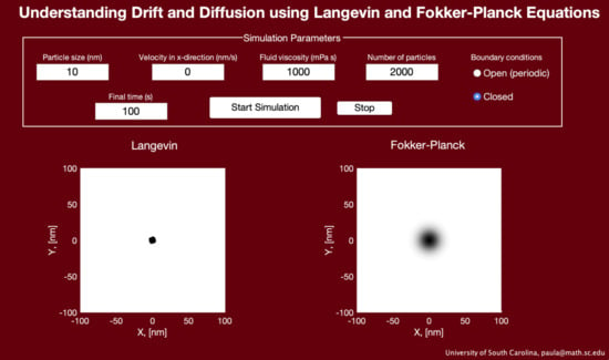
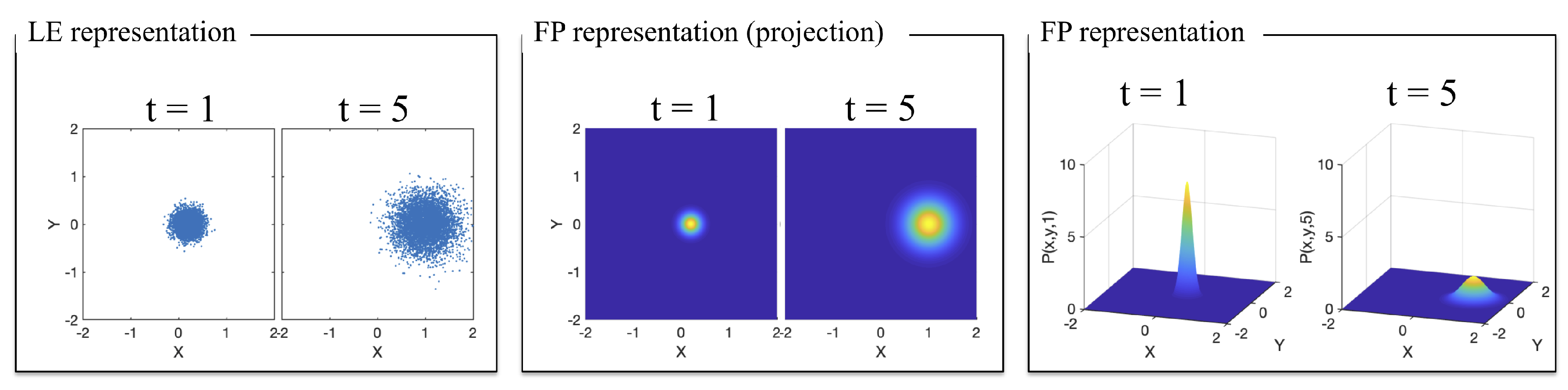
To elucidate the relation between these two types of approaches, Figure 1 shows the relation between a LE and a FP description of particles moving as a result of simple Brownian motion in two dimensions. This process describes the random migration of small particles arising from their motion due to thermal energy. The term Brownian motion was coined after the botanist Robert Brown, who was the first to describe this phenomenon in 1828 during his investigation of the movements of fine particles, like pollen, dust, and soot, on a water surface. In 1905, Albert Einstein explained Brownian motion in terms of random thermal motions of fluid molecules bombarding the microscopic particle and causing it to undergo a random walk [1]. Nonetheless, the range of applications of Brownian motion goes beyond the study of microscopic particles and includes modeling of thermal noise, stock prices, and random perturbations in many physical, biological, and economic systems [2,3]. From an observational point of view, the Langevin equation is easier to understand than the Fokker–Planck equation. The LE approach directly uses the concept of time evolution of the random variable describing the process; in the case of Figure 1, this corresponds to the individual particle’s position. In contrast, the FP approach follows the time evolution of the underlying probability distribution. That is, instead of describing a particle position, it describes the likelihood of finding a particle at a given position.
In this paper, we briefly describe the basics of LE equations and investigate their relation with their corresponding FP equations. The special cases discussed in the following sections are aimed at understanding how information is represented under these two different descriptions and illustrating how one can gather data under one approach and be able to infer behavior under the other.
2. Langevin Approach
To understand the Langevin description, we start by considering a particle immersed in a fluid. The particle “feels” a force arising from the collisions with the fluid’s molecules. This force consists of two parts: (a) a deterministic hydrodynamic drag, which resists motion; and (b) a fluctuating stochastic force, caused by thermal fluctuations. Newton’s second law gives the evolution equation governing the dynamics of the particle as
Assuming a linear drag force (force = −drag coefficient × velocity) and a white noise, the resulting equation is known as the Langevin equation:
White noise describes a random term that assumes no correlation on the fluctuating forces; this is captured by drawing a random number from a Gaussian distribution with mean and variance given by
where represents the variance of the distribution or strength of the noise; indicate vector components; is the Kronecker delta; and is a Dirac delta function. Note that both the Kronecker delta and Dirac delta function capture the zero-correlation of the forces both spatial, for , and temporal, for . Moreover, for any interval contained in interval , we have the following rule:
Since represents a stochastic term, Equation (1) is part of a broad class of differential equations known as stochastic differential equations (SDEs) [3,4].
Assuming white noise, one can solve Equation (1) formally using basic solution techniques for ordinary differential equations (ODEs). In particular, Equation (1) can be treated as a first order, non-homogeneous differential equation of the form
with integrating factor and solution given by
For Equation (1), , and , so that its formal solution is given by
The quantity has units of time and is usually referred to as the Brownian relaxation time of the particle velocity.
Note that, in the absence of random noise, , Equation (3) gives , which implies that as . However, according to the equipartition theorem, the velocity should satisfy
where the brackets represent averages; is the Boltzmann’s constant; T is the temperature; ; and d represents the degrees of freedom, or dimensionality, or 3. The fact that the equipartition theorem states that the velocity cannot approach zero as time goes to infinity implies that the random force is necessary to obtain the correct equilibrium condition. Furthermore, the strength of the noise, , should be such that equipartition theorem is satisfied.
To determine the strength of the random force, , we take the average of using Equation (3) as
In the last step of Equation (4), we used the property of the Dirac delta function given in Equation (2). Taking the limit as in Equation (4), and comparing it to the condition given by the equipartition theorem, gives
Therefore, the strength of the noise should satisfy
This relation between the strength of the fluctuations of the stochastic forces () and the dissipative term given by the drag force () is a special case of a more general result known as the fluctuation–dissipation theorem [5].
The fluctuation–dissipation theorem states that equilibrium is brought about by a dissipation force, in our case drag, between the particle and the medium, and whatever the mechanism of the dissipation, it has to be the same process that produces random, fluctuating forces on the particle. In other words, both the frictional force and the random force must be related since they have the same origin: fluid molecules “bombarding” the particle and inducing mobility.
Finally, after solving Equation (1), the particle position can be obtained as
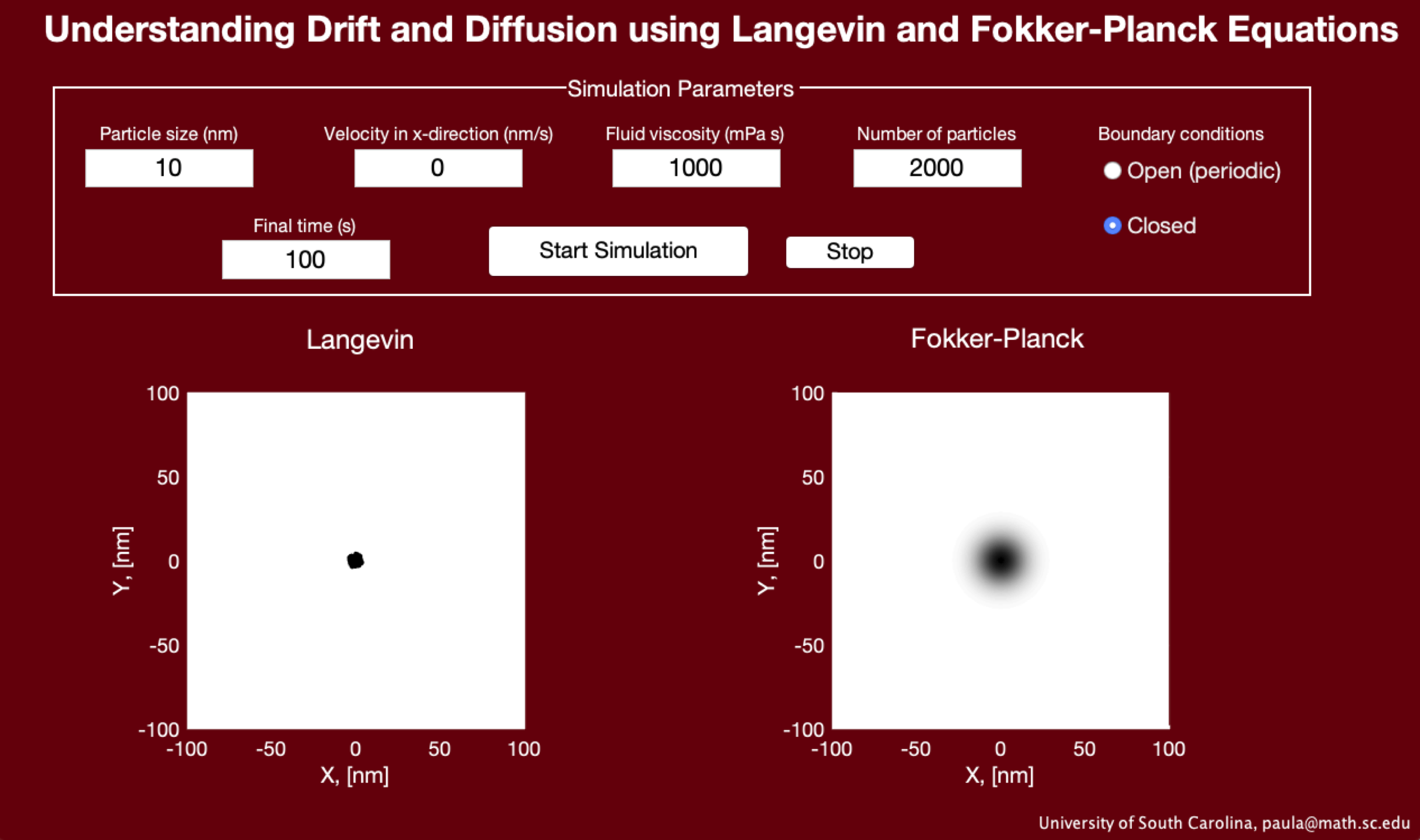
For a given SDE such as Equation (1), in order to make inferences based on its solution, it is necessary to find the average over many realizations. To illustrate this, consider the 2D version of Equation (1) solved three different times using the same initial position but subject to different random noises. The resulting trajectories are shown in Figure 2.
The fact that each trajectory is very different from the others implies that we cannot infer any behavior from the system by just considering a handful of solutions. That is, just as one would not be able to determine whether a coin is fair by just a couple of tosses, to be able to infer behavior based on Equation (1) one needs to look at many realizations of particle trajectories. This can be done numerically by solving the equation many times and then finding the average of such solutions or can be done analytically by using time-correlation functions, as discussed next.
2.1. Moments of a Stochastic Process
In mathematical statistics, the moment of a set of stochastic observations is defined as
Note that in the present application, our variables denote displacement of the particle with respect to the zero-time position, and the different moments measure deviations of the observations from the mean of the values. Within the context of fluid dynamics and Langevin equations, we are interested in the first () and second () moments of the particle positions. That is, the mean value of the stochastic variable and its spread or variance with respect to the mean.
- First momentFor the velocity in Equation (3), taking into account that , the mean is given bywith a long-time or equilibrium value given byFor the particle position,In addition, its long-time behavior is
- Second momentFrom Equation (4), the second moment for the velocity isFor the particle position, we haveIn this derivation, we have again used Equation (2) and the properties of the Dirac-delta function. For clarity, we solve each integral separately:Substituting and into the equation for givesThe quantity is called a mean squared displacement (MSD) and represents the square of the mean distance a particle has traveled in a given time interval. In practice, the MSD is one of the most commonly used experimental measures to determine material properties, as discussed in the next section.
2.2. Applications of the MSD
Performing a Taylor expansion of the MSD about gives
that is, at short times, the MSD grows quadratically in time. Similarly, at large times, we obtain
Using the definition of ,
where we have introduced the diffusion coefficient, .
The result in Equation (8) constitute a powerful tool in the characterization of fluids. The diffusion coefficient characterizes the mobility of particles of a given size in a given medium at a given temperature. For example, for spherical particles the drag coefficient is given by , where a is the particle radius and is the viscosity of the fluid. By embedding spherical particles in a fluid of unknown properties, one can estimate the viscosity of the fluid based on the particle trajectories.
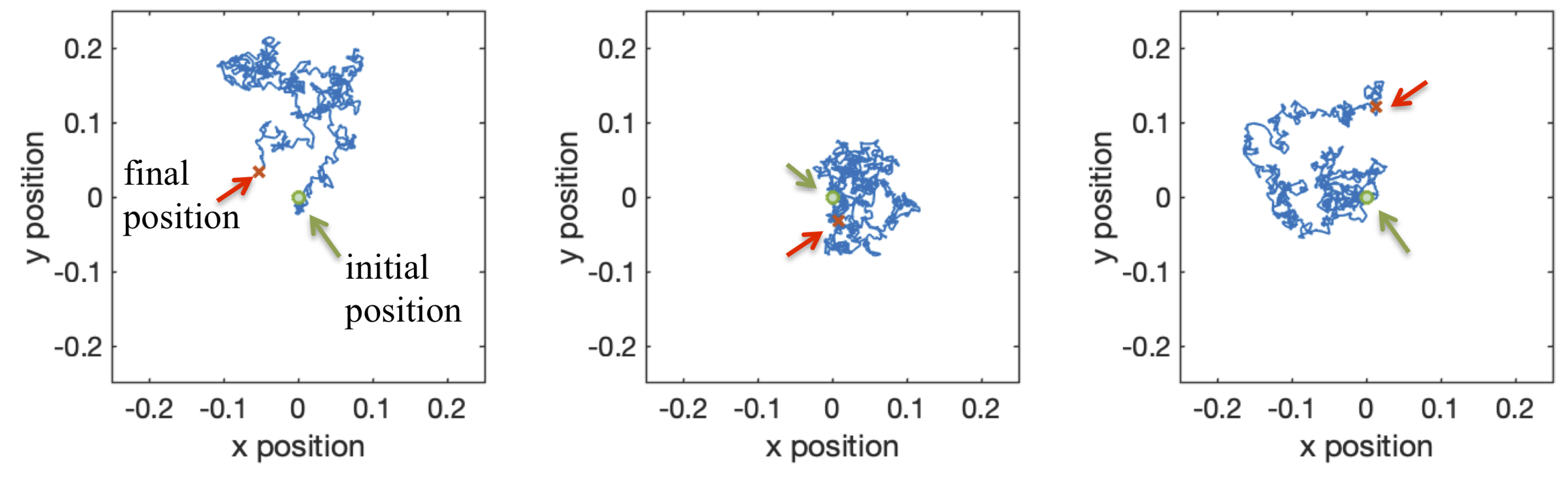
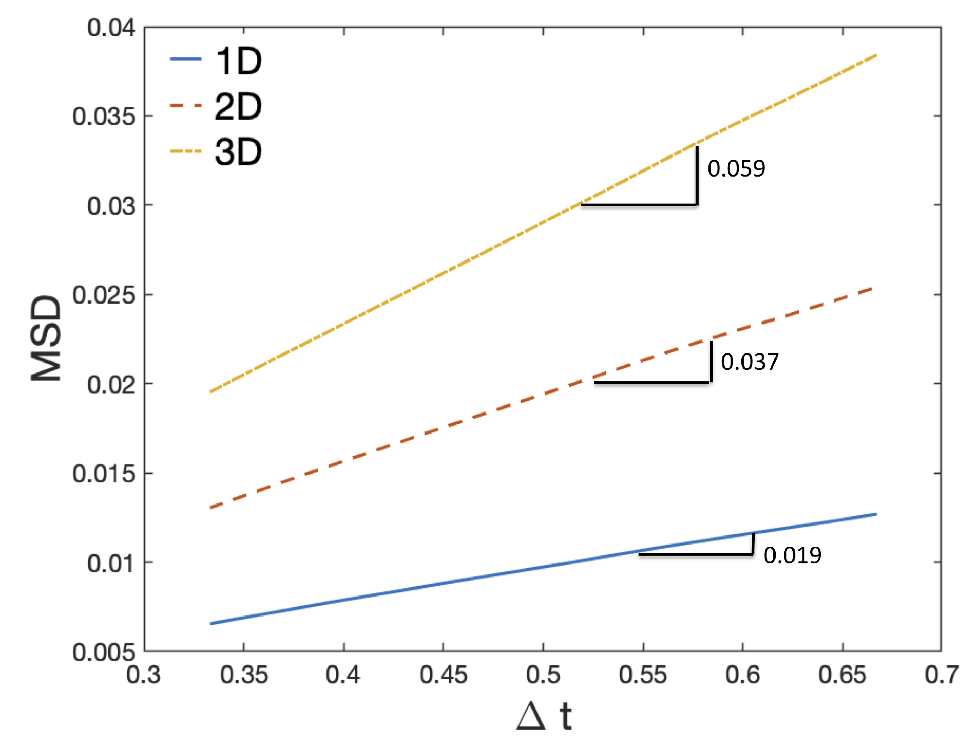
Assume we had tracked the trajectories of n spherical particles diffusing in a Newtonian fluid, , where . We can calculate the 1D, 2D, and 3D MSD as follows:
Examples of these MSDs are shown in Figure 3 for different ’s and the Matlab code used to generate them can be found in Appendix A. Note that in Appendix A we have used the zero-mass limit of the LE equation, see Section 2.4 for details of this limiting case.
Once the diffusion coefficient is found from the particle trajectories and the MSD, the fluid viscosity can be determined by
This type of inference can also be used with more complex fluids and/or different types of particles. For instance, the Einstein–Smoluchowski–Sutherland relation states that [6]
where is the particle’s mobility. This mobility is given by Stokes’ law in terms of the particle hydrodynamic radius, ,
where both the constant c and depend on the particle size and shape. Note that, for spherical particles, we return to the so called Stokes–Einstein relation,
however, the relation in Equation (9) stills holds for non-spherical particles.
In addition, complex fluids, such as viscoelastic materials, exhibit MSDs that do not depend linearly on time [7,8]. For example, the long-time MSD of some fluids obeys
This type of behavior is known as anomalous diffusion and the power law exponent, , indicates the type of diffusion: for , it is called subdiffusion, for , regular diffusion, and for , superdiffusion [9]. Although Equation (9) no longer holds in this case, material properties can still be inferred from the MSD of these fluids as discussed in [7,8].
2.3. Generalized Langevin Equations (GLE)
The GLE, as its name implies, is a generalization of Equation (1) and it can be similarly derived from Newton’s second law assuming that the forces acting over the particle are a stochastic force, a drag force, and some external conservative force [3]:
In the GLE approach, the drag coefficient is considered dynamic, so that the drag force is given by [5]
where is a memory kernel.
Since the external force is considered conservative, from Vector Calculus we know that this implies it arises from some potential field , such that
The resulting equation of motion is
The power of the GLE is that it is able to coarse-grain several degrees of freedom by describing: (i) explicitly the dynamics of variables of interests, which in this case corresponds to the position of a particle of mass m; and (ii) implicitly the remaining degrees of freedom through a memory kernel , a random noise , and an external potential . For free diffusion, particle mobility is in response only to stochastic thermal forces, i.e., , but in more complex systems external forces also play a role, .
The memory kernel, , represents a retarded effect of the frictional force, and to generate the correct equilibrium statistics, the random noise has to be related to this kernel in order to obey the fluctuation–dissipation theorem:
Physically, the kernel represents the fact that the medium requires a finite time to respond to any fluctuations in the motion of the particle; this in turn affects how the medium acts back on the particle. Thus, the force that the medium exerts on the particle at a given time depends on what the particle did in the past.
For simple fluids and large Brownian particles, the medium is capable of responding infinitely quickly to changes in the particle position, i.e., it has no memory. In this case the memory kernel is a delta-function and Equation (10) reduces to the Langevin equation previously discussed [3,5]:
Another extreme is a very sluggish medium that responds slowly to changes in the particle position. In this case, one can assume , so that the GLE becomes
thus adding an extra harmonic term to the potential. Such a term has the effect of trapping the system of particles in certain regions of its configuration space, an effect known as dynamic caging [10].
2.4. Zero-Mass Limit of the Langevin Equation
We finish this section on Langevin-type equations with a simplification. If we assume , and that the particles are so small that their mass is negligible, we obtain the so-called zero-mass limit:
This limit is also known as the overdamped or inertialess limit since it assumes that the inertial forces, , are negligible compared to the other forces acting on the particle. Rearranging terms and recalling that gives
where is a normally distributed random noise with and . For simplicity, in the following sections, we only consider the relation between equations of the form (14) and their respective Fokker–Planck equations.
3. Fokker–Planck Equation
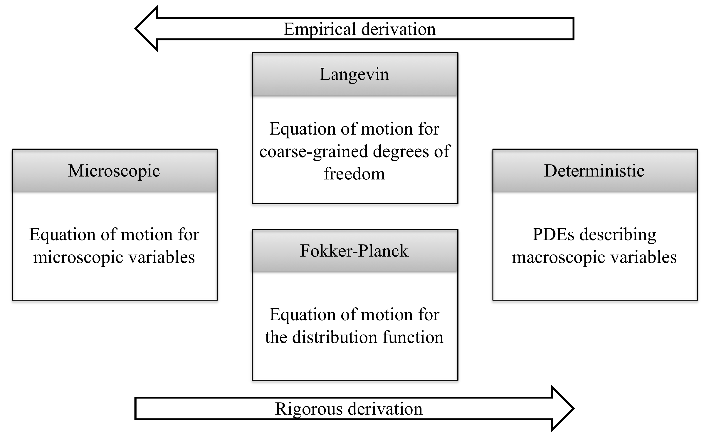
As discussed in the previous section, when a system is described by an LE, a complete description of the macroscopic system will require the solution and averaging of many SDEs. An equivalent approach is to describe the system by macroscopic variables which fluctuate as a result of stochasticity, instead of describing the individual evolution of stochastic probes [11]. An excellent explanation of the different representations and their characteristics can be found in Risken’s book [11], which we summarize in Figure 4.
A Fokker–Planck (FP) equation is a partial differential equation that describes the evolution of the probability density function (PDF) of a stochastic variable. For Langevin-type equations of the form given by Equation (14), the stochastic variable is a particle’s position as a function of time, . The corresponding PDF is the function that gives the probability of a particle being in the position at time t as . The reader is referred to Appendix B for a brief introduction to PDFs.
Note that taking a deterministic perspective is equivalent to ignoring the random noise term in the LE, , which results in the absence of the diffusion term in the FP equation, . This simple statement helps us identify the relation between fluctuations at the microscale and diffusion at the macroscale. That is, the observed diffusion at the macroscale is the result of fluctuations arising from the fluid’s molecules bombarding the probe at the microscale.
3.1. One-Dimensional Examples
In the following examples, we assume that all initial positions of particles are located at zero, that is,
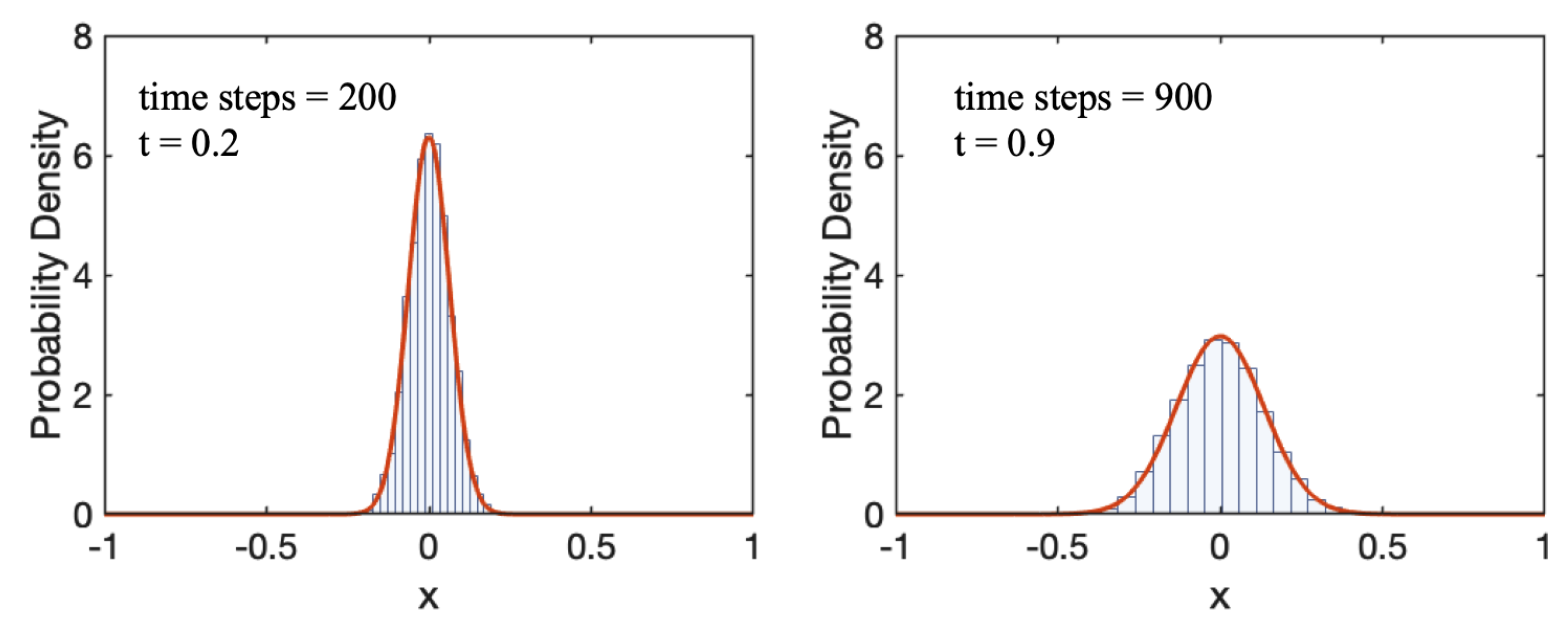
- Brownian motion without external field for small particles ()In this case, the corresponding FP equation is the well-known diffusion equation, which has the same mathematical form of the heat equation in the context of heat transfer under temperature gradients:We can find the general solution of this equation using similarity solutions with the transformationwhere represents temporal decay and is a shape factor used to reduce the partial differential equation (PDE) to an ordinary differential equation (ODE). For details on how this particular form is obtained, the reader is referred to [12].We can calculate the derivatives of using Equation (18) asSubstituting in Equation (17) givesSince we have yet to define a value for p, we conveniently choose it to be , so that the two quantities in the parenthesis are the same. Finally, a solution for the resulting differential equation will satisfywith the general solutionwhich gives the solution for ,To find the value of the constant of integration , we consider the fact thatthat is, all possible realizations are included, see Appendix B.To solve the integral, we introduce the error functionwhich has values and .which givesTherefore, the solution of the FP equation iswhich is a one-dimensional Gaussian function centered at zero: and with variance .To compare these results with those obtained in the LE section, we consider the first and second moments of .The first moment is given byWe use integration by substitution () to obtainandFor the second moment, we havewhich is the same result we obtained in the limit for Equation (8), when the dimensionality is .Solutions at different times are shown in Figure 5, together with the normalized histograms obtained from LE data. For details of the histogram normalization see Appendix B.
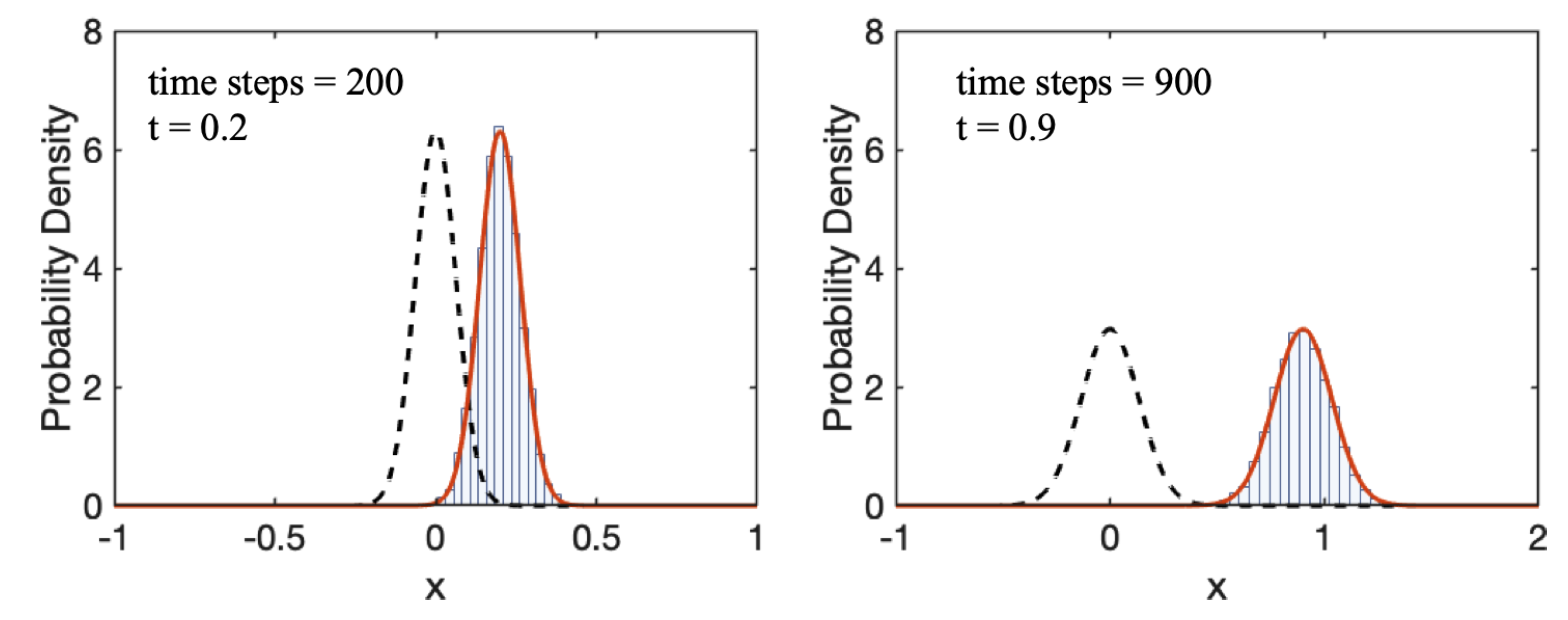
- Brownian motion with external field for small particles ()A common example of an external field is a background velocity, u, which imposes a drift on the particles:The corresponding FP equation is the advection–diffusion equationThe solution of this PDE is [13]A comparison between Equations (19) and (22) shows that the only difference between these two solutions is in a “shift” of x by . That is, the effect of drift is to move the mean of the Gaussian distribution from zero.As before we can calculate the first and second moment of the distribution function as [13]That is, the mean position of the particle is displaced by the background velocity over a distance . In addition, note that the MSD at long times becomes due to the additional linear flow in the fluid.In the case of simple diffusion, the dispersion of the particles can be attained from the MSD or equivalently the variance of the Gaussian. In the case where drift is present, dispersion is superimposed by the background flow, for this reason a more accurate measure of the dispersion is given by the metric [13]which gives back the linear behavior characteristic of standard diffusive processes. Note that in this equation, is a central moment as opposed to the general definition given at the beginning of Section 2.1. These two moments will coincide if the mean is zero.
3.2. Two-Dimensional Examples
In this section, we present the 2D equations corresponding to four different cases and their numerical solutions.
- No external field
- -
- Langevin equationsIn this case, both and are statistically independent white noises; the subscripts are used to denote that the noise histories are for x and y.
- -
- Fokker–Planck Equation
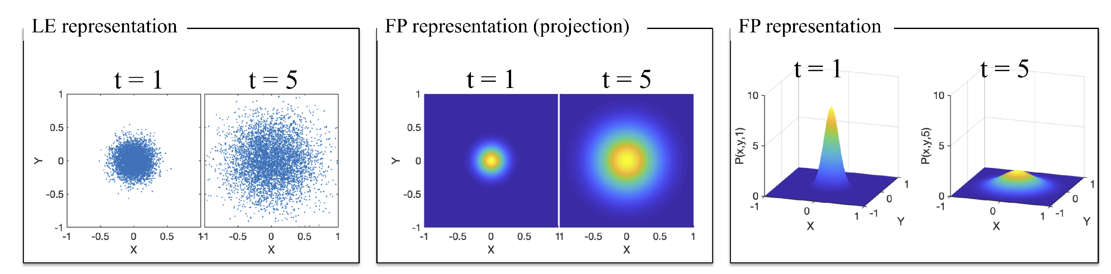
Solutions for LE and FP representations for this case of no external field are provided in Figure 7.Note that, in two dimensions, we obtain two LEs, but still one FP equation. In general, as the degrees of freedom of the system increase, the choice between LE and FP representations is analogous to the choice between solving many SDEs and solving a single, high-dimensional PDE. - Constant drift in the x-direction,
- -
- Langevin equations
- -
- Fokker–Planck Equation
Solutions for LE and FP representations for this case of constant drift in the x-direction are provided in Figure 8. - Background flow field,For any background field of the form where and are constants,the Langevin equations are given byThis equation can be written in vector form aswhere is the strain-rate tensor. The corresponding FP equation isNote that when , the equations reduce to those for constant drift, as discussed above.
- -
- Example: simple shear,
- *
- Langevin equations
- *
- Fokker–Planck Equation
Solutions for LE and FP representations for this case of simple shear flow are provided in Figure 9.
4. Conclusions
In this paper, we analyzed the relation between Langevin (LE) and Fokker–Planck (FP) representations of particles moving in a fluid due to Brownian motion with and without external fields. Although each description offers a different perspective of the underlying fluid dynamics, there is a direct connection between these two approaches, which were explored through simple examples in both one and two dimensions. In studying these two families of equations, we employed subjects from calculus, such as Taylor expansions and conservative vector fields; ordinary differential equations, such as integrating factors; and partial differential equations, such as similarity solutions.
The LE representation involves stochastic differential equations (SDEs) and offers the advantage of allowing the microscopic process to be easily incorporated into the equations. One of the drawbacks of this representation is that it is necessary to have as many SDEs as degrees of freedom in the system and each SDE needs to be solved many times to reduce statistical noise.
The FP approach involves a partial differential equation (PDE) describing the evolution of the probability density function (PDF) of the stochastic variable. Unlike numerical solutions for SDEs, which are noisy, solutions for the FP are deterministic and as such can truly avoid noise. One of its drawbacks is that the dimensionality of the PDF increases with the number of degrees of freedom of the system, which leads to high algorithmic complexity, and as a result, the corresponding numerical schemes have a high computational cost.
Experimentally, LE equations can be informed by techniques that capture the movement of probes at the microscale such as passive microrheology [8]. On the other hand, FP equations can be informed by experimental techniques that capture the behavior of the ensemble of probes such as light scattering experiments [14].
Author Contributions
Conceptualization, A.M. and P.A.V.; methodology, A.M. and P.A.V.; software, A.M., R.D. and P.A.V.; validation, A.M., R.D. and P.A.V.; formal analysis, A.M. and P.A.V.; investigation, A.M. and P.A.V.; resources, P.A.V.; data curation, P.A.V.; writing—original draft preparation, A.M., R.D. and P.A.V.; writing—review and editing, A.M. and P.A.V.; visualization, A.M., R.D. and P.A.V.; supervision, P.A.V.; project administration, P.A.V.; funding acquisition, P.A.V. All authors have read and agreed to the published version of the manuscript.
Funding
This research was funded by National Science Foundation, grant number NSF-DMS 1751339 and NASA, grant number 80NSSC19K0159 P00004.
Conflicts of Interest
The authors declare no conflict of interest.
Appendix A
| %% Constants D = 1e—2; % diffusion coefficient dt = 1e—3; % time step Np = 5e2; % number of particles NT = 1e3; % number of time steps %% Generate particle positions x = zeros(Np,NT); y = zeros(Np,NT); z = zeros(Np,NT); for k=2:NT x(:,k) = x(:,k—1) + sqrt(2*D*dt)*randn(Np,1); y(:,k) = y(:,k—1) + sqrt(2*D*dt)*randn(Np,1); z(:,k) = z(:,k—1) + sqrt(2*D*dt)*randn(Np,1); end %% Calculate MSD lag = round((1/3)*NT):round((2/3)*NT); for k=1:length(lag) dx = x(:,1+lag(k):end)—x(:,1:end—lag(k)); dy = y(:,1+lag(k):end)—y(:,1:end—lag(k)); dz = z(:,1+lag(k):end)—z(:,1:end—lag(k)); msd1(k,:) = mean(dx’.^2); msd2(k,:) = mean(dx’.^2+dy’.^2); msd3(k,:) = mean(dx’.^2+dy’.^2+dz’.^2); end %% Plot MSDs plot(lag*dt,mean(msd1’),’linewidth’,3) hold on plot(lag*dt,mean(msd2’),’—’,’linewidth’,3) plot(lag*dt,mean(msd3’),’–.’,’linewidth’,3) %% Recover D fmsd1 = fit(lag’*dt,mean(msd1’)’,’a*x’,’start’,1); fmsd2 = fit(lag’*dt,mean(msd2’)’,’a*x’,’start’,1); fmsd3 = fit(lag’*dt,mean(msd3’)’,’a*x’,’start’,1); fmsd1.a/2 fmsd2.a/4 fmsd3.a/6 |
Appendix B
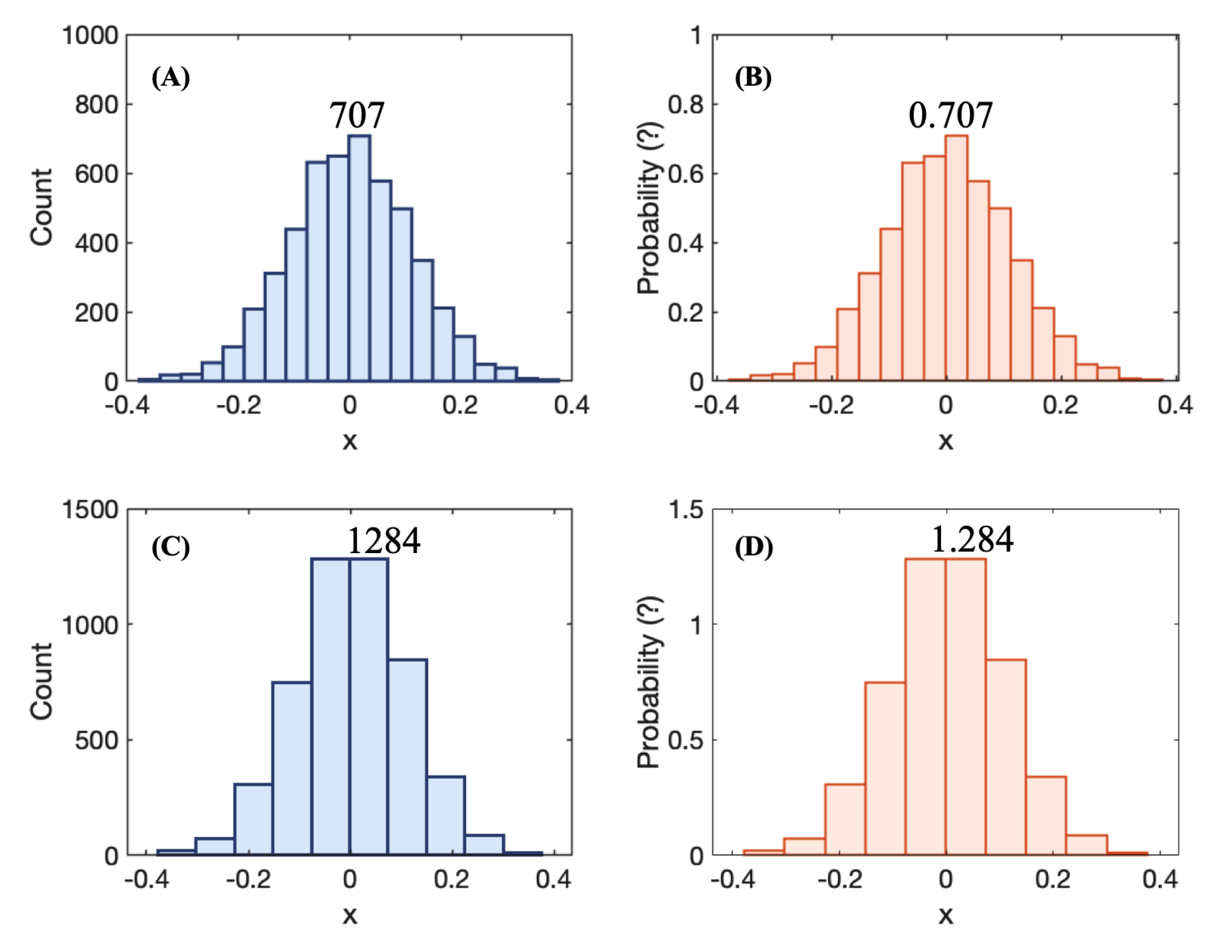
Recall that in Figure 2, the trajectory of three different particles were plotted. Assume we are interested in determining the x-coordinate of the final position of a particle. From the figure, we would have three different answers: , , and . It is clear that the fact that each plot gives a different answer is a result of the randomness of the process. This simple observation implies that the correct question is not what is the position of the particle? but rather what is the most likely position of the particle? To answer this, we collect the final position of 1000 particles and summarize them using histograms, like the ones shown in Figure A1.
To construct histograms, we divide the data into groups or ‘bins’ and count how many realizations fall within each bin. The next question is how to extract probabilities out of these histograms. A first attempt to calculate probabilities is to divide the number of realizations within each bin by the total number of realizations. An inspection of Figure A1 shows why this is not the correct approach; although both figures (B) and (D) correspond to the same data, the answer is different depending on the number of bins used.
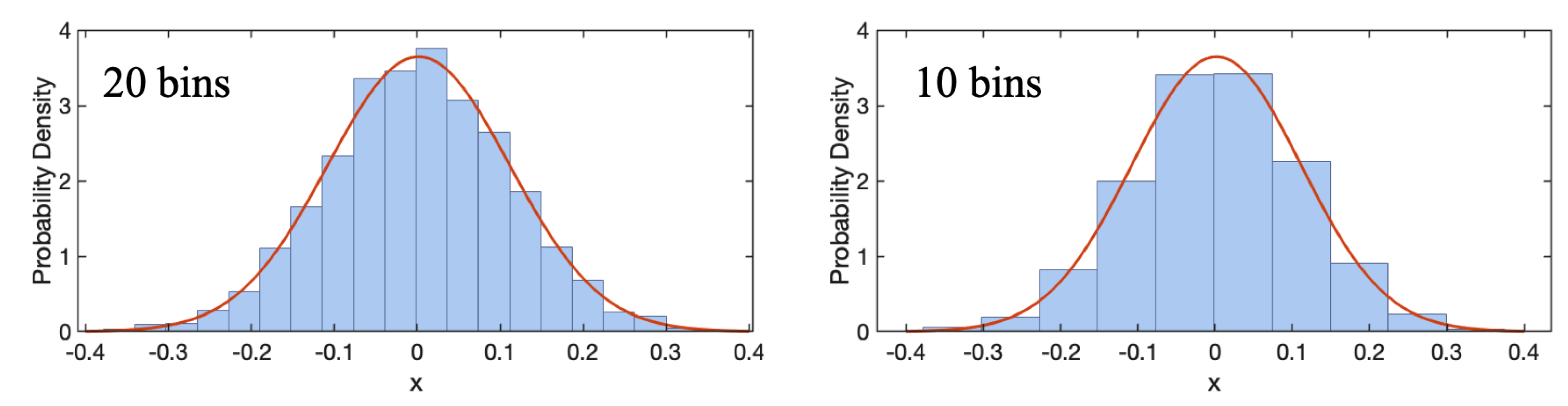
In order to transform the histogram data into probabilities, it is necessary to eliminate the effect of the bin size. This is done by normalizing the histogram using the area of each bin, rather than the counts in each bin. This normalization is shown in Figure A2.
Figure A1.
Histograms of particle positions for 1000 particles. (A) counts using 20 bins; (B) counts from (A) divided by total number of particles; (C) counts using 10 bins; (D) counts from (C) divided by total number of particles.
Figure A1.
Histograms of particle positions for 1000 particles. (A) counts using 20 bins; (B) counts from (A) divided by total number of particles; (C) counts using 10 bins; (D) counts from (C) divided by total number of particles.

Figure A2.
Normalized histogram of particle positions. The code used to generate these plots can be found in Appendix B.
Figure A2.
Normalized histogram of particle positions. The code used to generate these plots can be found in Appendix B.

Since the size of the bins does not affect the resulting plot, we could make the size of the bins as small as we wish, to the point of being able to trace a continuous probability density function, represented by the continuous line in Figure A2, which is unique to the data independently of the number of bins used.
Just as its name indicates, a PDF is not exactly a probability. However, just as one can find the mass of an object by multiplying its density by its volume, we can find a probability by multiplying is probability density (PDF) by a range. In this sense, the quantity
represents the probability that a particle’s position is in the range at time t.
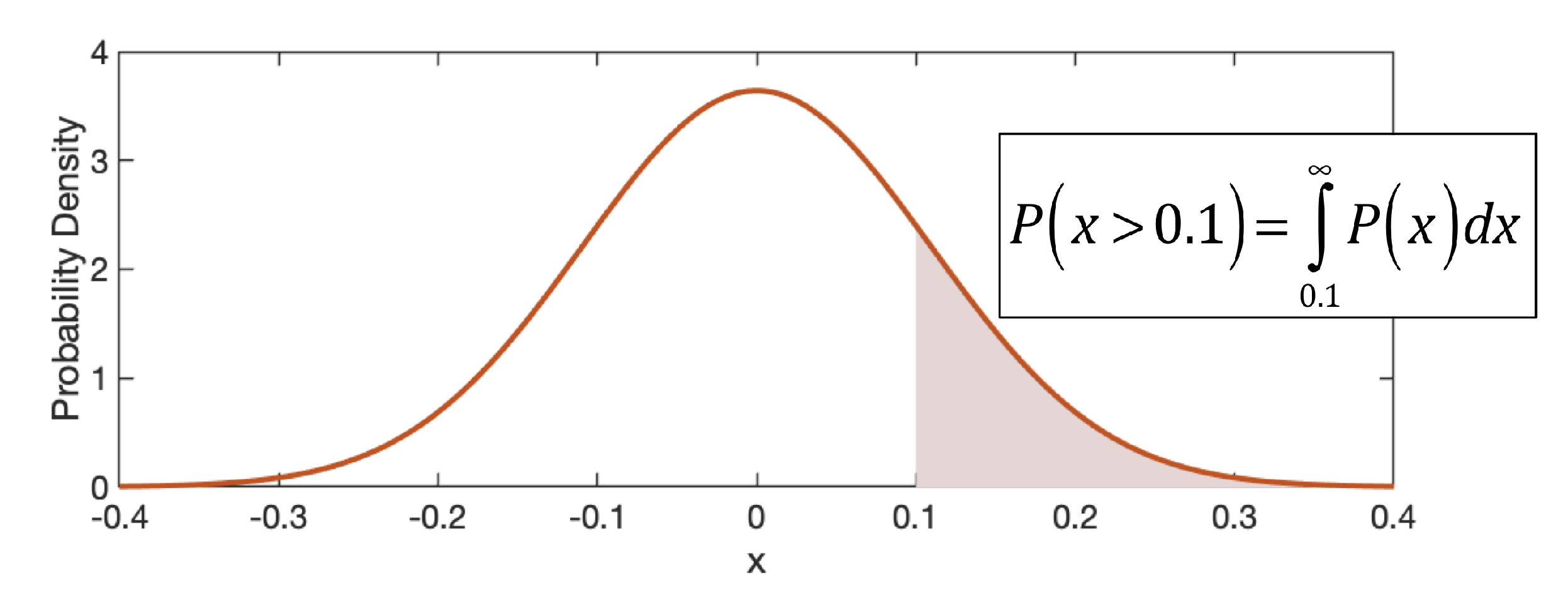
In addition, working with the continuous form of the PDF, , allows us to use integrals to find different probabilities as areas under the curve, as the example given in Figure A3, or to provide a definition of statistical moments based on PDFs:
Figure A3.
Calculating probabilities using PDFs.

Note that since the area under the PDF should represent all possible realizations, we have the condition that the area under the whole curve should be equal to one:
As a final remark, note that not all PDFs are bell-shaped like a Gaussian. The only condition that remains true for all PDFs is that the area under the curve is equal to one as defined in Equation (A1). In addition, not all PDFs have to define a probability density for every location of the sample space. For a more in-depth review of different probability distribution functions, the reader is referred to [15].
| %% Computing and Normalizing histogram [c,n] = hist(x(:,600),20); c1 = c./trapz(n,c); %% Fitting to normal distribution [mu,sigma,muci,sigmaci] = normfit(x(:,600)); Y = normpdf(linspace(−0.4,0.4,1e3),mu,sigma); %% Plots bar(n,c1) hold on plot(linspace(−0.4,0.4,1e3),Y) |
References
- Einstein, A. Uber die von der molekularkinetischen Theorie der Warme geforderte Bewegung von in ruhenden Flussigkeiten suspendierten Teilchen. Annalen der Physik 1905, 322, 49–560. [Google Scholar] [CrossRef] [Green Version]
- Karatzas, I.; Shreve, S.E. Brownian Motion and Stochastic Calculus; Springer: New York, NY, USA, 1998. [Google Scholar]
- Coffey, W.; Kalmykov, Y.P. The Langevin Equation: With Applications to Stochastic Problems in Physics, Chemistry and Electrical Engineering; World Scientific: Singapore, 2012; Volume 27. [Google Scholar]
- Arnold, L. Stochastic Differential Equations: Theory and Applications; John Wiley and Sons: New York, NY, USA, 1974. [Google Scholar]
- Kubo, R. The fluctuation-dissipation theorem. Rep. Prog. Phys. 1966, 29, 255. [Google Scholar] [CrossRef] [Green Version]
- March, N.H.; Tosi, M.P. Introduction to Liquid State Physics; World Scientific: Singapore, 2002. [Google Scholar]
- Mason, T.G.; Ganesan, K.; Van Zanten, J.H.; Wirtz, D.; Kuo, S.C. Particle tracking microrheology of complex fluids. Phys. Rev. Lett. 1997, 79, 3282. [Google Scholar] [CrossRef] [Green Version]
- Furst, E.M.; Squires, T.M. Microrheology; Oxford University Press: Oxford, UK, 2017. [Google Scholar]
- Klafter, J.; Blumen, A.; Shlesinger, M.F. Stochastic pathway to anomalous diffusion. Phys. Rev. A 1987, 35, 3081. [Google Scholar] [CrossRef] [PubMed]
- Tuckerman, M. Statistical Mechanics: Theory and Molecular Simulation; Oxford University Press: Oxford, UK, 2010. [Google Scholar]
- Risken, H. Fokker-Planck Equation; Springer: Berlin/Heidelberg, Germany, 1996. [Google Scholar]
- Renardy, M.; Rogers, R.C. An Introduction to Partial Differential Equations; Springer Science & Business Media: Berlin/Heidelberg, Germany, 2006. [Google Scholar]
- Codling, E.A.; Plank, M.J.; Benhamou, S. Random walk models in biology. J. R. Soc. Interface 2008, 25, 813–834. [Google Scholar] [CrossRef] [PubMed]
- Sarmiento-Gomez, E.; Santamaria-Holek, I.; Castillo, R. Mean-square displacement of particles in slightly interconnected polymer networks. J. Phys. Chem. B 2014, 118, 1146–1158. [Google Scholar] [CrossRef] [PubMed]
- Evans, M.J.; Rosenthal, J.S. Probability and Statistics: The Science of Uncertainty; Macmillan: New York, NY, USA, 2004. [Google Scholar]
Figure 1.
Relation between the Langevin equations (LE) and Fokker–Planck (FP) solutions. (A) LE solutions give particle positions as functions of time, each point represents a particle position at some time t. All particles have initial position and follow different trajectories dictated by their respective noise history. (B) The distribution of particle positions can be summarized using a histogram. (C) FP solutions shows the probability of finding a particle at a given position as a function of time; darker color indicates a higher probability of finding a particle at that position.

Figure 2.
Evolution of 2D particle position for three different solutions of Equation (1). All three trajectories start from an initial position . In all three figures, = 0.001 and the simulation ran for 1000 time steps.
Figure 2.
Evolution of 2D particle position for three different solutions of Equation (1). All three trajectories start from an initial position . In all three figures, = 0.001 and the simulation ran for 1000 time steps.

Figure 3.
Mean squared displacement (MSD) in 1D, 2D, and 3D. Each line has been fitted to a function of the form , the best fitting value for the slope m is shown for each line. The slope for 1D is , giving , the slope for 2D gives , and for 3D it is . As a reference, the diffusion coefficient used to generate the particle trajectories is .

Figure 4.
Levels of description of a system, adapted from [11].
Figure 4.
Levels of description of a system, adapted from [11].

Figure 5.
Probability density function (PDF) for position of particles diffusing via one-dimensional Brownian motion. Histograms correspond to LE data and solid lines corresponds to FP solutions. In this figure, m/s.
Figure 5.
Probability density function (PDF) for position of particles diffusing via one-dimensional Brownian motion. Histograms correspond to LE data and solid lines corresponds to FP solutions. In this figure, m/s.

Figure 6.
PDF for position of particles diffusing via one-dimensional Brownian motion plus drift. Histograms correspond to generalized Langevin equations (GLE) data and solid lines corresponds to FP solutions. For comparison, FP solutions without drift are shown in dashed lines. In this figure, m/s, /s.

Figure 7.
LE and FP solutions for two-dimensional Brownian motion without external field. For both representations, m/s and time is in seconds. For the LE representation, the total number of particles is .
Figure 7.
LE and FP solutions for two-dimensional Brownian motion without external field. For both representations, m/s and time is in seconds. For the LE representation, the total number of particles is .

Figure 8.
LE and FP solutions for two-dimensional Brownian motion with constant drift. For both representations, m/s, /s and time is in seconds. For the LE representation, the total number of particles is .
Figure 8.
LE and FP solutions for two-dimensional Brownian motion with constant drift. For both representations, m/s, /s and time is in seconds. For the LE representation, the total number of particles is .

Figure 9.
LE and FP solutions for two-dimensional Brownian motion with simple shear flow. For both representations, m/s, /s and time is in seconds. For the LE representation, the total number of particles is .
Figure 9.
LE and FP solutions for two-dimensional Brownian motion with simple shear flow. For both representations, m/s, /s and time is in seconds. For the LE representation, the total number of particles is .

© 2020 by the authors. Licensee MDPI, Basel, Switzerland. This article is an open access article distributed under the terms and conditions of the Creative Commons Attribution (CC BY) license (http://creativecommons.org/licenses/by/4.0/).
Share and Cite
MDPI and ACS Style
Medved, A.; Davis, R.; Vasquez, P.A. Understanding Fluid Dynamics from Langevin and Fokker–Planck Equations. Fluids 2020, 5, 40. https://0-doi-org.brum.beds.ac.uk/10.3390/fluids5010040
AMA Style
Medved A, Davis R, Vasquez PA. Understanding Fluid Dynamics from Langevin and Fokker–Planck Equations. Fluids. 2020; 5(1):40. https://0-doi-org.brum.beds.ac.uk/10.3390/fluids5010040
Chicago/Turabian StyleMedved, Andrei, Riley Davis, and Paula A. Vasquez. 2020. "Understanding Fluid Dynamics from Langevin and Fokker–Planck Equations" Fluids 5, no. 1: 40. https://0-doi-org.brum.beds.ac.uk/10.3390/fluids5010040