Time-Dependent Motion of a Floating Circular Elastic Plate


School of Mathematical and Physical Sciences, The University of Newcastle, Callaghan, NSW 2308, Australia
Fluids 2021, 6(1), 29; https://0-doi-org.brum.beds.ac.uk/10.3390/fluids6010029
Submission received: 16 December 2020
/
Revised: 6 January 2021
/
Accepted: 6 January 2021
/
Published: 8 January 2021
(This article belongs to the Special Issue Mathematical and Numerical Modeling of Water Waves)
Abstract
:The motion of a circular elastic plate floating on the surface is investigated in the time-domain. The solution is found from the single frequency solutions, and the method to solve for the circular plate is given using the eigenfunction matching method. Simple plane incident waves with a Gaussian profile in wavenumber space are considered, and a more complex focused wave group is considered. Results are given for a range of plate and incident wave parameters. Code is provided to show how to simulate the complex motion.
1. Introduction
The single frequency solution for the linear water wave problem is extensively used to model the hydroelastic response of very large floating structures, container ships, or an ice floe [1,2,3,4]. The simplest example problem in hydroelasticity is the floating elastic plate, which has been the subject of extensive research. Many different methods of solution have been developed, including Green function methods [5,6], eigenfunction matching [7,8,9], multi-mode methods [10] and the Wiener–Hopf method [11,12].
The problem becomes more complicated if we consider the time-dependent problem. If the floating plate is assumed to be of infinite extent, the problem becomes simpler and a spatial Fourier transform gives the solution [13,14,15,16,17,18,19]. The forced vibration of a finite floating elastic plate was solved by [20] using a variational formulation and the Rayleigh–Ritz method. The problem was analyzed in shallow water by [21,22,23] and in finite depth by [24]. The solution for incident waves in two-dimensions was given in finite depth by [25,26,27] and in shallow water in two by [21,22] and three–dimensions by [23]. A comparison for the time–dependent motion in two-dimensions for an initial condition was given in [28]. The solution for finite water depth in three–dimensions was found by [29,30,31,32] and was experimentally investigated by [33]. The solution due to a transient incident wave forcing was given in [34]. Recently, there has been extensive work on nonlinear simulations using computational fluid dynamics to investigate nonlinear phenomena [35,36,37,38]. However, even for the case of high amplitude waves, the linear wave problem remains valid for a floating plate [39], and this model continues to the basis of offshore engineering and scattering by an ice floe.
The eigenfunction matching method has been applied to many floating elastic plate problems. It has proved to give the most uncomplicated solutions, provided that the geometry is sufficiently simple that it can be applied. The solution method was first described in [7] and this is where the solution of the special dispersion equation for a floating elastic plate was introduced. This method was extended to circular [9], multiple [40,41,42], and submerged elastic plates [43,44].
We present here a solution to the time-dependent problem of a floating circular plate subject to incident wave forcing. In part, the purpose of this work is to show how simply the complex time-domain motion of such systems can easily be computed using the frequency-domain solution. We also extend the formulation to a focused incident wavepacket. The outline is as follows. In Section 2, we derive the equations of motion in the time and frequency domain. In Section 3, we show how the solution can be found using eigenfunction matching in the frequency domain. In Section 4, we illustrate how the solution in the time domain can be found straightforwardly from the frequency domain solutions.
We acknowledge that much of the material presented here has appeared in various previous works. In particular, the eigenfunction matching for a circular plate which underlies the calculations presented here. However, the present work aims to show how the time-domain solution can be found straightforwardly from the frequency domain solution. In some sense, the floating elastic plate is just a beautiful example to illustrate this method. We have given sufficient details of the solution method to understand the code that accompanies the paper. We also note that the code which accompanies this work is an essential part of it, and this has not been made available previously.
2. Equations of Motion
We consider here a floating elastic plate of uniform thickness and negligible draft. The plate is assumed to be circular with radius a. The fluid is of constant depth H with the z axis pointing vertically up and the free surface at . Such a plate has been the subject of extensive research. The displacement of the plate is denoted by w and the spatial velocity potential for the fluid by . The equation The plate has a uniform thickness h. This uniform thickness floating plate model has been the validated by laboratory experiments [45,46]. It reduces to that of a rigid body in the case of long waves.
We begin by stating the governing equations for the plate–water system, which was discussed in detail in [47], assuming that the equation of linear water waves governs the problem. The kinematic condition is
where w is the displacement of the fluid surface (which is also the plate displacement for ) and is the velocity potential of the fluid. The dynamic condition is
where is the water density, g is the gravitational acceleration, E is the Young’s modulus of the plate, is its Poisson’s ratio, and is its density. Laplace’s equation applies throughout the fluid
and the usual non-flow condition at the bottom surface
Assuming that all motions are time harmonic with radian frequency , the velocity potential of the water, , can be expressed as
where the reduced velocity potential is complex-valued, and is the horizontal spatial variable.
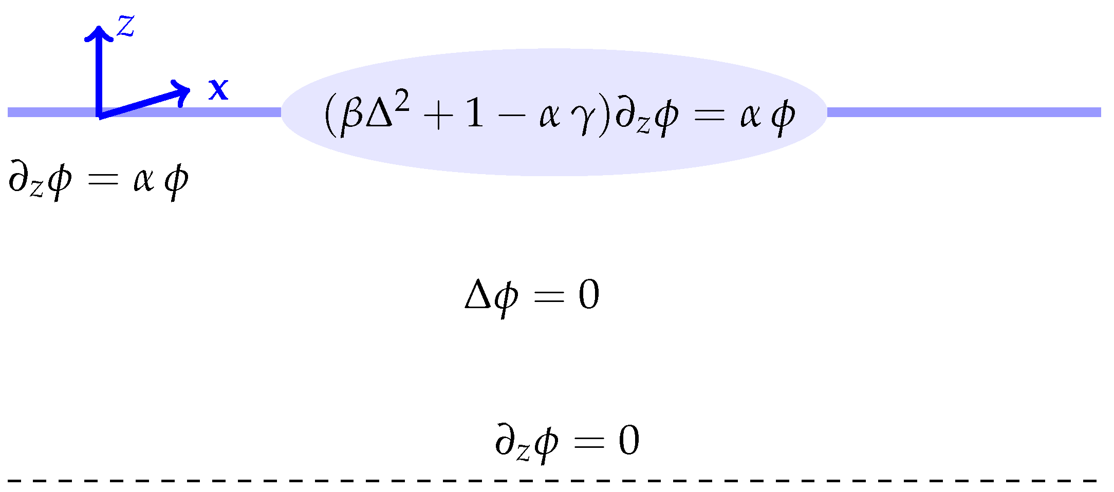
The frequency-domain potential satisfies the boundary value problem
where is the Laplacian operator in the horizontal plane. The constant and and are
The free plate boundary conditions and the radiation condition need to be applied. Figure 1 gives a schematic diagram of the problem.
3. Eigenfunction Matching
We derive the solution by the eigenfunction matching method here. The solution in two-dimensions first appeared in [7] and the three–dimensional solution was given in [9]. We begin by separating variables and writing
Applying Laplace’s equation, we obtain
so that
where the separation constant must satisfy the standard dispersion equations
Note that we have set under the free surface and under the plate. The dispersion equations are discussed in detail in [7]. We denote the negative imaginary solution of (11) by and the positive real by , . The solutions of (12) are denoted by , . The fully complex with positive real part are and (where ), the negative imaginary is and the positive real are , . We define
as the vertical eigenfunction of the potential in the open water region and
as the vertical eigenfunction of the potential in the plate covered region.
We now use circular symmetry to write
where are the polar coordinates in the direction. We now solve for the function . Using Laplace’s equation in polar coordinates, we obtain
where is or depending on whether r is greater or less than a. We can convert this equation to the standard form by substituting to obtain
The solution of this equation is a linear combination of the modified Bessel functions of order n, and . Since the solution must be bounded, we know that under the plate it will be a linear combination of while outside the plate will be a linear combination of . Therefore, the potential can be expanded as
where and are the coefficients in the open water and the plate covered region, respectively.
The incident potential is a wave of amplitude A in displacement travelling in the positive x-direction. Following [8], it can be written as
where .
The boundary conditions for the plate also have to be considered. The vertical force and bending moment must vanish, which can be written as
and
where w is the time-independent surface displacement, is Poisson’s ratio, and is the in polar coordinates is
The surface displacement and the velocity potential at the water surface are linked through the kinematic boundary condition
The relationship between the potential and the surface displacement is
The surface displacement can also be expanded in eigenfunctions as
using the fact that
The boundary conditions (21) and (22) can be expressed in terms of the potential using (28). Since the angular modes are uncoupled, the conditions apply to each, giving
and
The potential and its derivative must be continuous across the transition from open water to the plate-covered region. Therefore, at they have to be equal. Again we know that this must be true for each angle and we obtain
and
for each n. We solve these equations by multiplying both by and integrating from to 0 to obtain
where
where
and
where
Equation (33) can be solved for the open water coefficients
which can then be substituted into Equation (34) to give us
for each n. Together with (29) and (30), (40) gives the required equations to solve for the coefficients of the water velocity potential in the plate covered region. For the numerical solution, we truncate the sum at N, and then we have equations from matching through the depth and two extra equations from the boundary conditions.
It should be noted that the solutions for positive and negative n are complex conjugates so that they do not both need to be calculated. There are some minor simplifications which are a consequence of this and are discussed in more detail in [8].
4. Time-Dependent Forcing and Numerical Results
We have denoted the surface displacement in the frequency domain is given by . However, the surface displacement is a function of and is a function of wavenumber k. We have also only considered waves incident from the positive x direction (. This choice of direction makes sense given the circular symmetry, but we can consider waves incident from other angles (found by rotation of the solution by the angle). Therefore, we denote the complex frequency domain surface displacement by .
4.1. Plane Incident Wave Forcing
The simplest time-dependent problem is to consider a place incident wave from the positive x direction. We assume that the incident wave is a Gaussian at . Therefore, the time–dependent displacement is then given by the following Fourier integral
where is
where is a scale factor and we set and is the central wavenumber, we set .
4.2. Focused Wave Group
It is more interesting to consider two-dimensional incident waves. A simple focused wave group can be constructed as from the following formula
where is another scaling parameters which we set to be
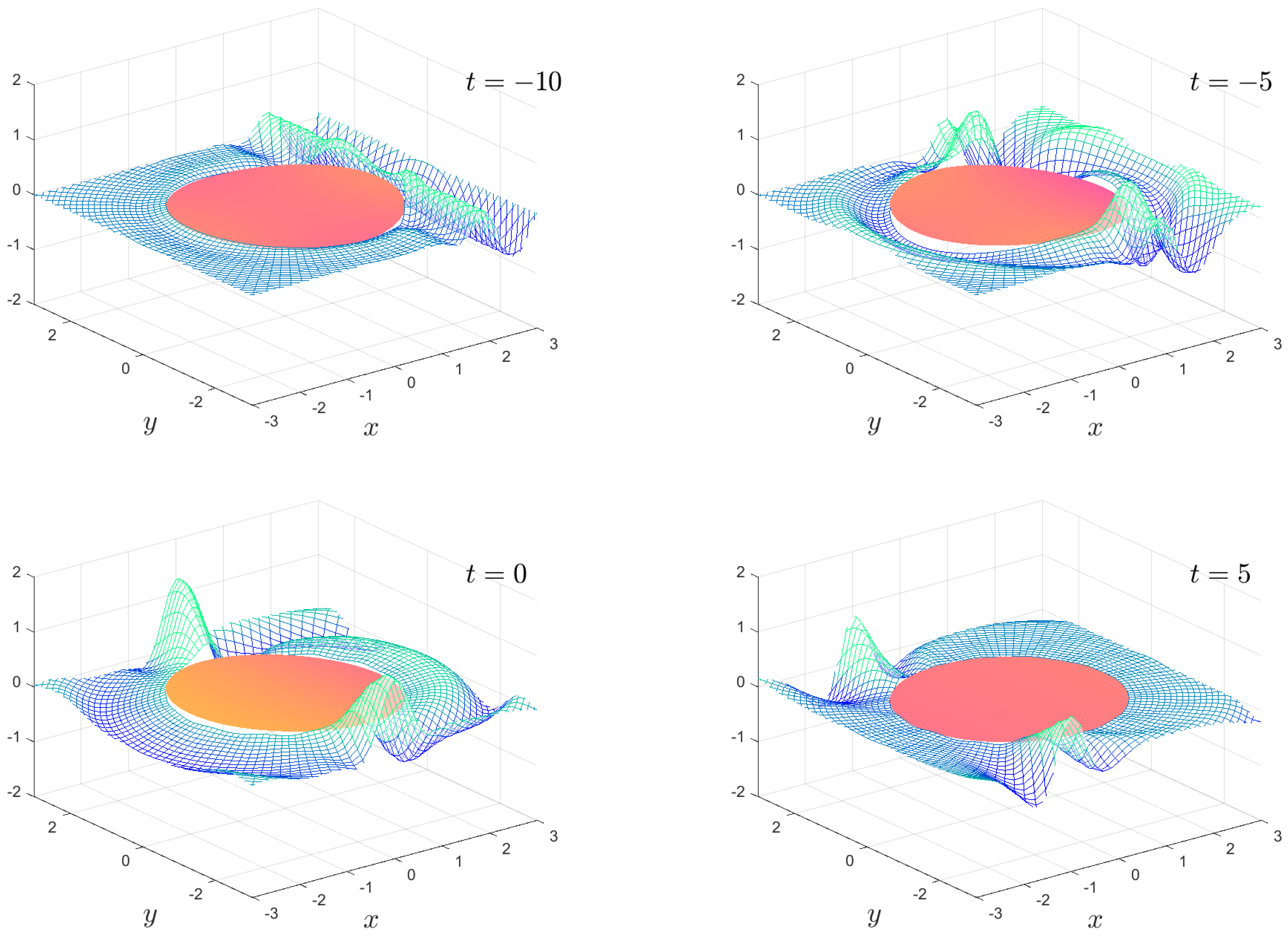
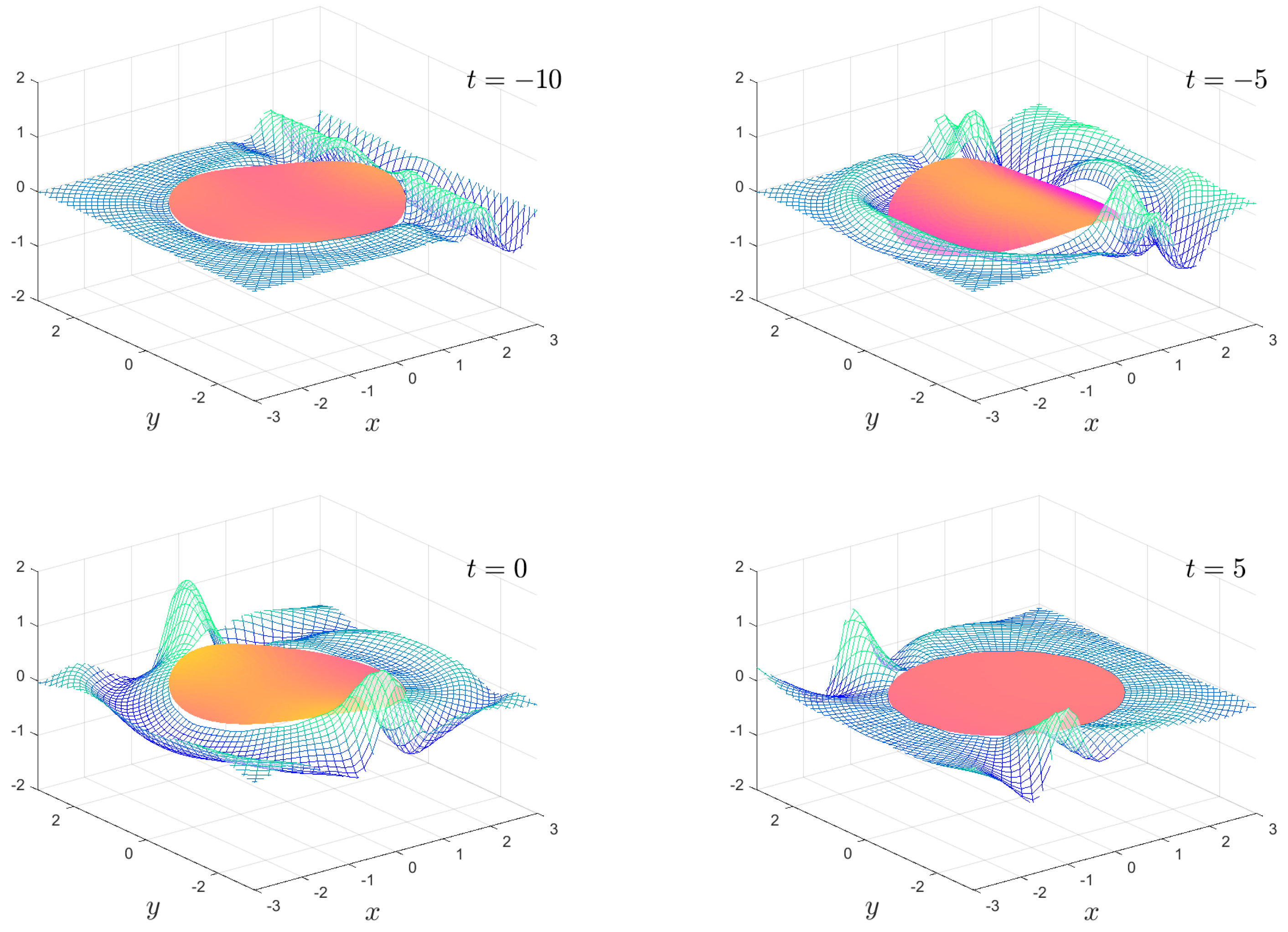
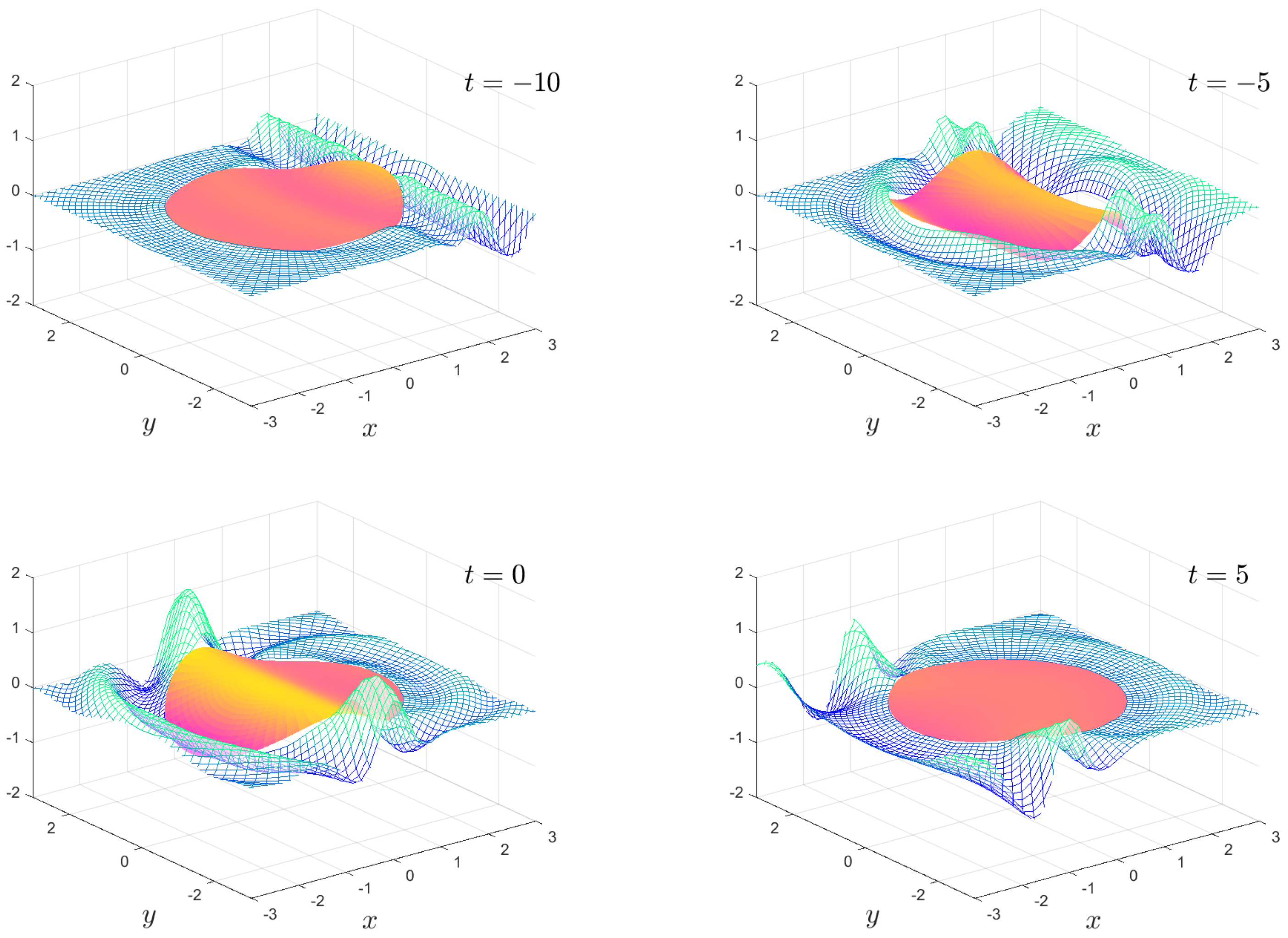
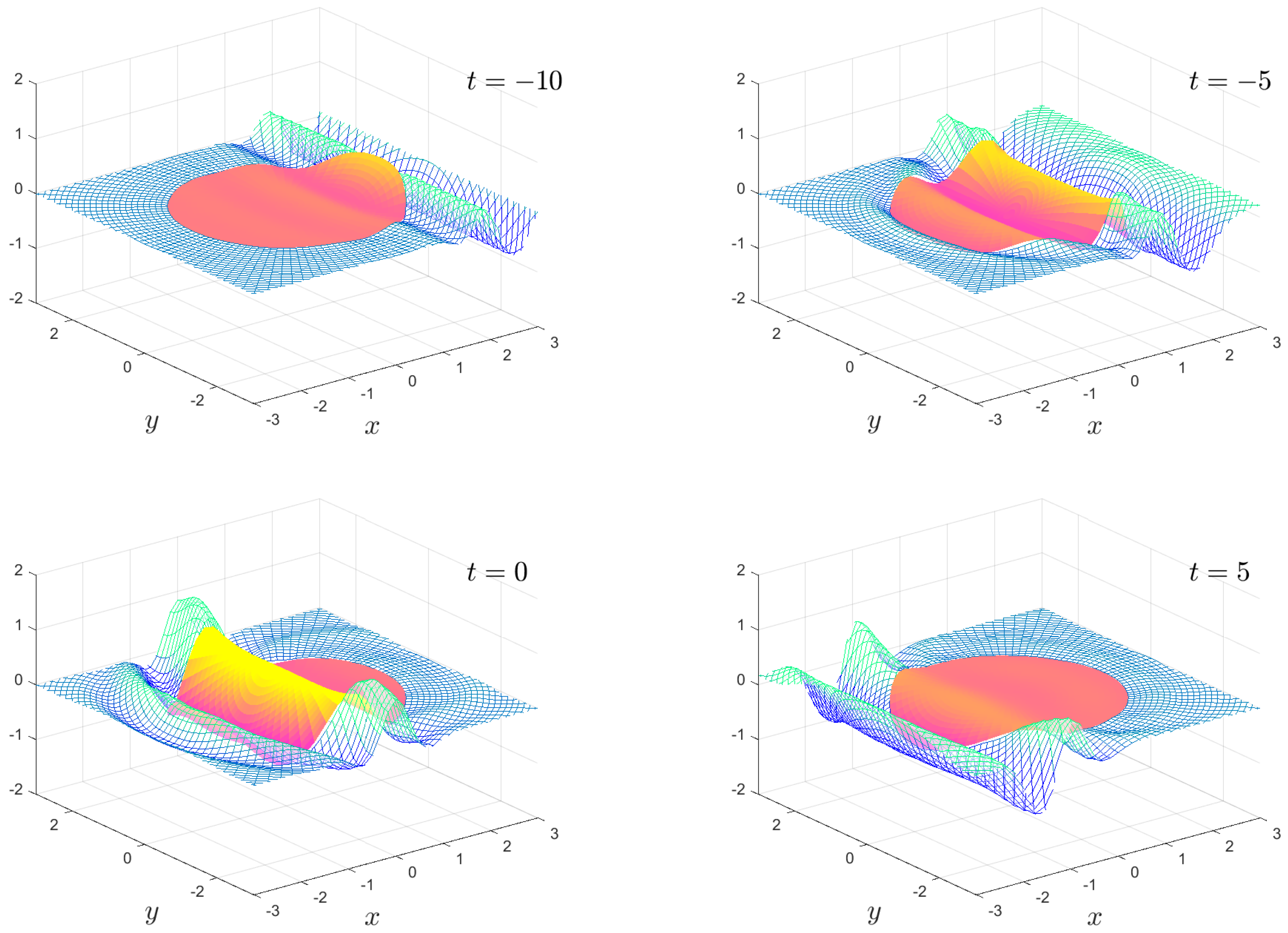
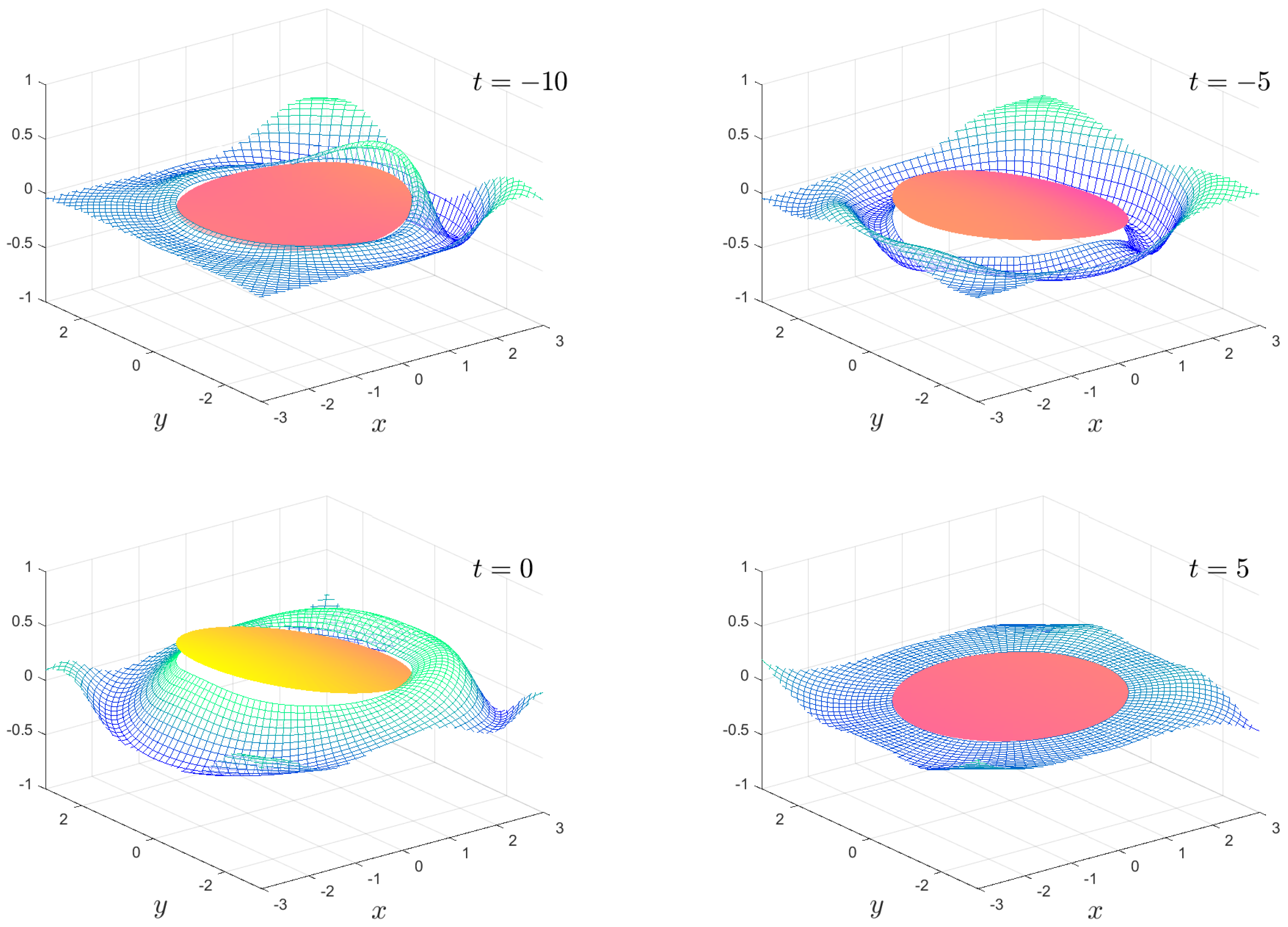
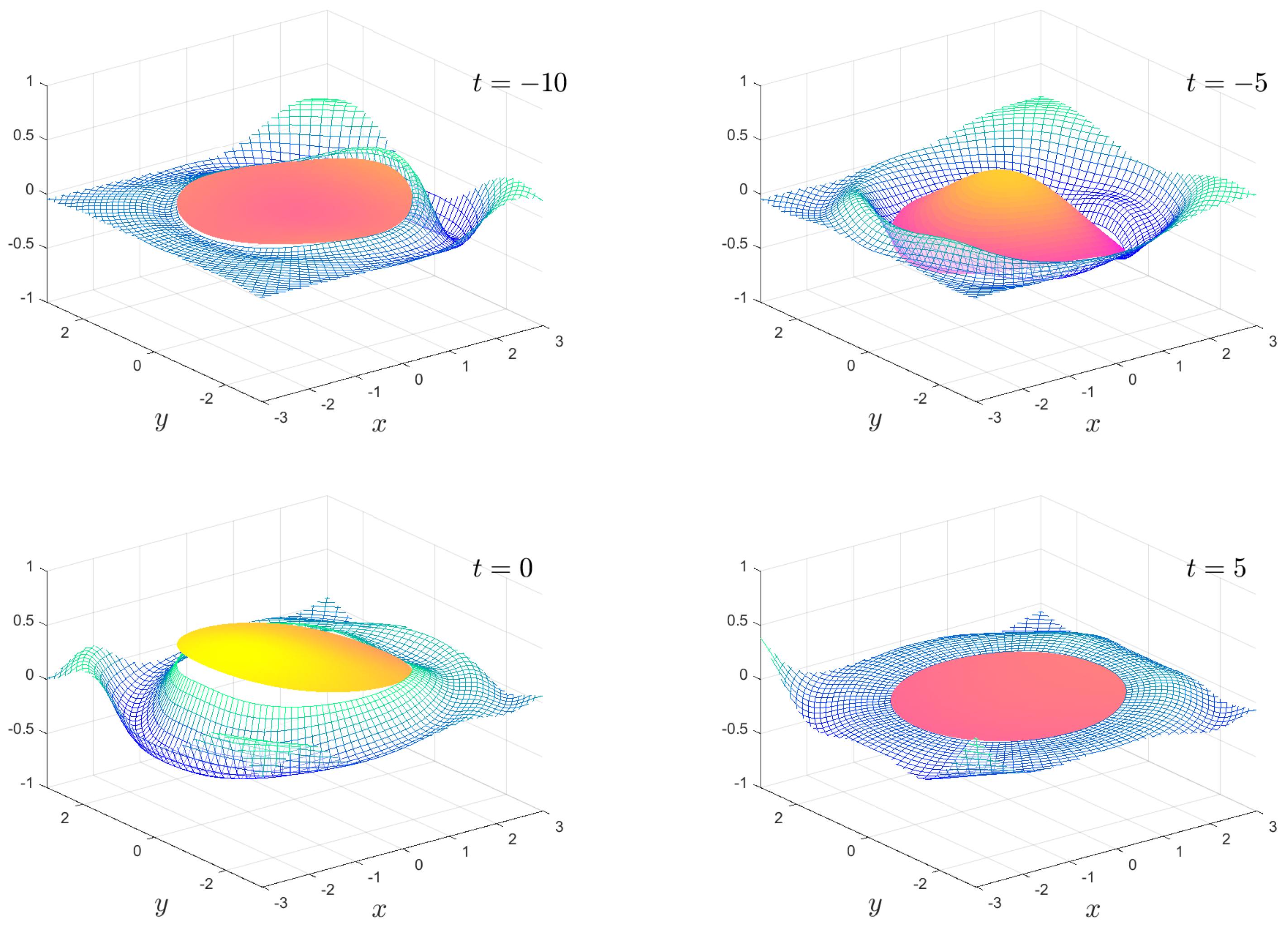
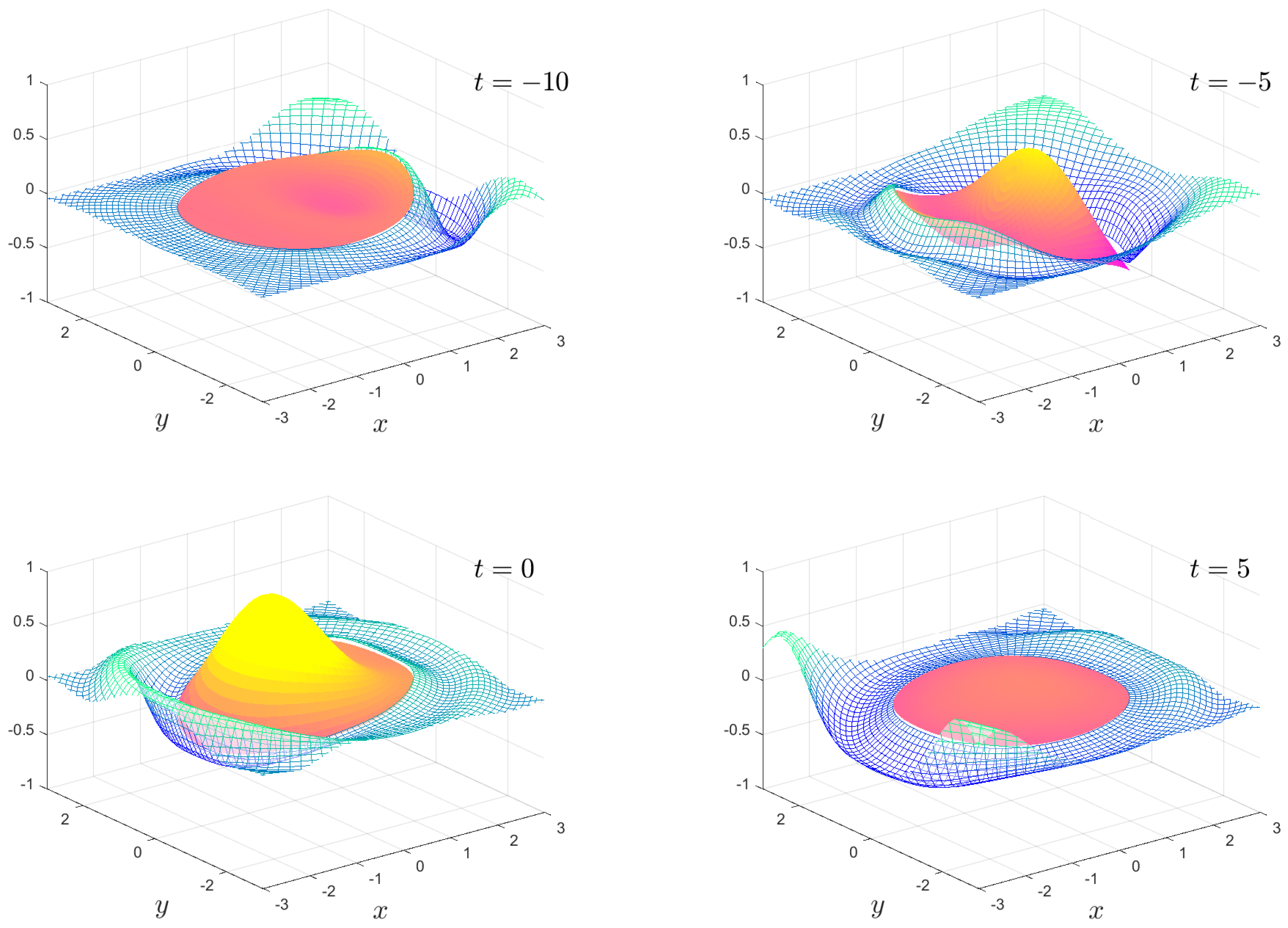
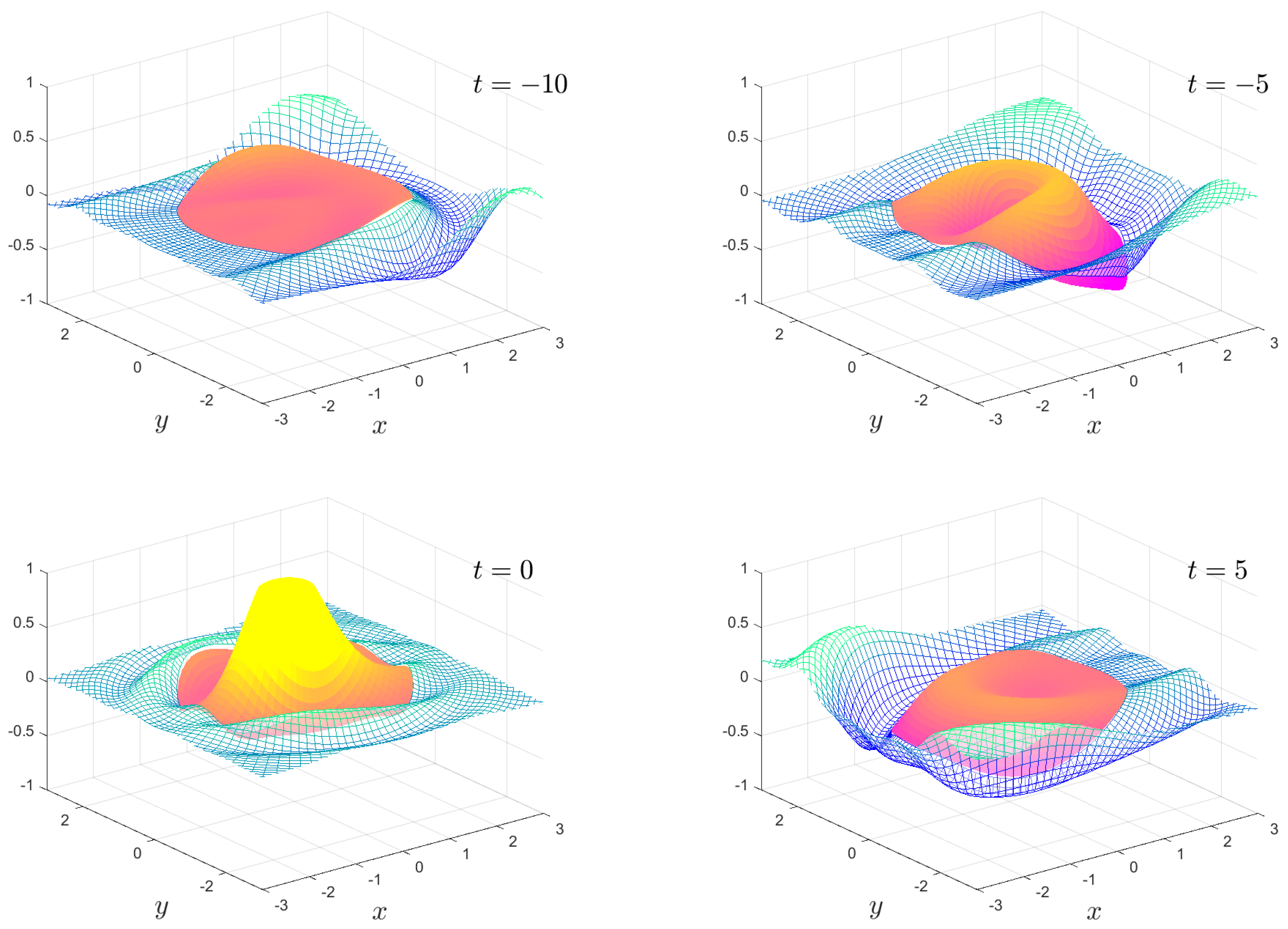
The numerical results we present are a subset of the possible motions which are possible. We fix the mass , the water depth and the floe radius for all calculations. The solution is shown as an animation in movies 1 to 8, which are given as Supplementary Material. Figure 2, Figure 3, Figure 4 and Figure 5 show snapshots from movies 1 to 4, respectively, for the times . We change the stiffness from in Figure 2 to in Figure 5. The plate goes from being virtually stiff to highly flexible. The complex motion of the plate and fluid systems can be seen, especially in the movies in the Supplementary Material.
Figure 6, Figure 7, Figure 8 and Figure 9 show the solution for the more complicated and interesting case of an incident wave packet. The complex and resonant behaviour of the plate and fluid system is clearly visible. In particular, the transition from the wave diffracting around the plate to the wave travelling under the plate as the stiffness transitions from high to low is visible. Moreover, we have an intermediate region where resonances exist, and the plate motion becomes highly complicated. The ability to visualise this motion offers insights which are not so easily obtained from the frequency domain solution.
5. Conclusions
The purpose of this work is to show how we can easily visualise the complex time-domain behaviour of complex wave scattering problems such as those which arise from the scattering by a flexible plate. While the frequency–domain solution is central to our calculations, the scattering results from the frequency domain solution are often challenging to interpret in the context of incident wave packets. By the simple visualisation using the suitable superposition of incident waves, we can bring the complex motion to life. The author hopes that these results, and the accompanying computer code, will encourage others to also investigate such visualisations for their complex water wave scattering problem.
Supplementary Materials
The following are available at https://0-www-mdpi-com.brum.beds.ac.uk/2311-5521/6/1/29/s1, The movie files and MATLAB code are provided as Supplementary Material.
Funding
This work is funded by the Australian Research Council (DP200102828).
Data Availability Statement
The MATLAB code to make the calculations is provided as Supplementary Material.
Conflicts of Interest
The author declares no conflict of interest.
References
- Bishop, R.E.D.; Price, W.G.; Wu, Y. A General Linear Hydroelasticity Theory of Floating Structures Moving in a Seaway. Philos. Trans. R. Soc. 1986, 316, 375–426. [Google Scholar]
- Kashiwagi, M. Research on Hydroelastic Response of VLFS: Recent Progressand Future Work. Int. J. Offshore Polar Eng. 2000, 10, 81–90. [Google Scholar]
- Squire, V.A. Synergies Between VLFS Hydroelasticity and Sea Ice Research. Int. J. Offshore Polar Eng. 2008, 18, 1–13. [Google Scholar]
- Watanabe, E.; Utsunomiya, T.; Wang, C.M. Hydroelastic analysis of pontoon-type VLFS: A literature survey. Eng. Struct. 2004, 26, 245–256. [Google Scholar] [CrossRef]
- Newman, J.N. Wave effects on deformable bodies. Appl. Ocean Res. 1994, 16, 45–101. [Google Scholar] [CrossRef]
- Meylan, M.H.; Squire, V.A. The Response of Ice Floes to Ocean Waves. J. Geophy. Res. 1994, 99, 891–900. [Google Scholar] [CrossRef]
- Fox, C.; Squire, V.A. On the Oblique Reflexion and Transmission of Ocean Waves at Shore Fast Sea Ice. Philos. Trans. R. Soc. Lond. A 1994, 347, 185–218. [Google Scholar]
- Zilman, G.; Miloh, T. Hydroelastic Buoyant Circular Plate in Shallow Water: A Closed Form Solution. Appl. Ocean Res. 2000, 22, 191–198. [Google Scholar] [CrossRef]
- Peter, M.A.; Meylan, M.H.; Chung, H. Wave scattering by a circular elastic plate in water of finite depth: A closed form solution. Int. J. Offshore Polar Eng. 2004, 14, 81–85. [Google Scholar]
- Bennetts, L.G.; Biggs, N.R.T.; Porter, D. A multi-mode approximation to wave scattering by ice sheets of varying thickness. J. Fluid Mech. 2007, 579, 413–443. [Google Scholar] [CrossRef]
- Balmforth, N.; Craster, R. Ocean waves and ice sheets. J. Fluid Mech. 1999, 395, 89–124. [Google Scholar]
- Chung, H.; Fox, C. Calculation of wave-ice interaction using the Wiener-Hopf technique. N. Z. J. Math. 2002, 31, 1–18. [Google Scholar]
- Davys, J.W.; Hosking, R.J.; Sneyd, A.D. Waves due to a Steadily Moving Source on a Floating Ice Plate. J. Fluid Mech. 1985, 158, 269–287. [Google Scholar] [CrossRef]
- Hosking, R.J.; Sneyd, A.D.; Waugh, D.W. Viscoelastic Response of a Floating Ice Plate to a Steadily Moving Load. J. Fluid Mech. 1988, 196, 409–430. [Google Scholar] [CrossRef]
- Milinazzo, F.; Shinbrot, M.; Evans, N.W. A Mathematical Analysis of the Steady Response of Floating Ice to the Uniform Motion of a Rectangular Load. J. Fluid Mech. 1995, 287, 173–197. [Google Scholar]
- Squire, V.A.; Hosking, R.J.; Kerr, A.D.; Langhorne, P.J. Moving Loads on Ice Plates; Kluwer: Alphen aan den Rijn, The Netherlands, 1996. [Google Scholar]
- Nugroho, W.; Wang, K.; Hosking, R.; Milinazzo, F. Time-dependent response of a floating flexible plate to an impulsively started steadily moving load. J. Fluid Mech. 1999, 381, 337–355. [Google Scholar]
- Wang, K.; Hosking, R.; Milinazzo, F. Time-dependent response of a floating viscoelastic plate to an impulsively started moving load. J. Fluid Mech. 2004, 521, 295–317. [Google Scholar] [CrossRef]
- Bonnefoy, F.; Meylan, M.; Ferrant, P. Nonlinear higher-order spectral solution for a two-dimensional moving load on ice. J. Fluid Mech. 2009, 621, 215–242. [Google Scholar]
- Meylan, M.H. The forced vibration of a thin plate floating on an infinite liquid. J. Sound Vib. 1997, 205, 581–591. [Google Scholar]
- Meylan, M.H. Spectral Solution of Time Dependent Shallow Water Hydroelasticity. J. Fluid Mech. 2002, 454, 387–402. [Google Scholar]
- Sturova, I.V. Unsteady behavior of an elastic beam floating on shallow water under external loading. J. Appl. Mech. Tech. Phys. 2002, 43, 415–423. [Google Scholar] [CrossRef]
- Sturova, I.V. The action of an unsteady external load on a circular elastic plate floating on shallow water. J. Appl. Maths Mechs. 2003, 67, 407–416. [Google Scholar] [CrossRef]
- Meylan, M.H. The time-dependent vibration of forced floating elastic plates by eigenfunction matching in two and three dimensions. Wave Motion 2019, 88, 21–33. [Google Scholar] [CrossRef]
- Tkacheva, L. Plane problem of vibrations of an elastic floating plate under periodic external loading. J. Appl. Mech. Tech. Phys. 2004, 45, 420–427. [Google Scholar] [CrossRef]
- Tkacheva, L. Action of a periodic load on an elastic floating plate. Fluid Dyn. 2005, 40, 282–296. [Google Scholar] [CrossRef]
- Hazard, C.; Meylan, M.H. Spectral theory for a two-dimensional elastic thin plate floating on water of finite depth. SIAM J. Appl. Math. 2007, 68, 629–647. [Google Scholar] [CrossRef]
- Meylan, M.H.; Sturova, I.V. Time-Dependent Motion of a Two-Dimensional Floating Elastic Plate. J. Fluid. Struct. 2009, 25, 445–460. [Google Scholar]
- Kashiwagi, M. A Time-Domain Mode-Expansion Method for Calculating Transient Elastic Responses of a Pontoon-Type VLFS. J. Mar. Sci. Technol. 2000, 5, 89–100. [Google Scholar] [CrossRef]
- Kashiwagi, M. Transient responses of a VLFS during landing and take-off of an airplane. J. Mar. Sci. Technol. 2004, 9, 14–23. [Google Scholar] [CrossRef]
- Qui, L. Numerical simulation of transient hydroelastic response of a floating beam induced by landing loads. Appl. Ocean Res. 2007, 29, 91–98. [Google Scholar]
- Matiushina, A.A.; Pogorelova, A.V.; Kozin, V.M. Effect of Impact Load on the Ice Cover During the Landing of an Airplane. Int. J. Offshore Polar Eng. 2016, 26, 6–12. [Google Scholar] [CrossRef]
- Endo, H.; Yago, K. Time history response of a large floating structure subjected to dynamic load. J. Soc. Nav. Archit. Jpn. 1999, 1999, 369–376. [Google Scholar] [CrossRef]
- Montiel, F.; Bennetts, L.; Squire, V. The transient response of floating elastic plates to wavemaker forcing in two dimensions. J. Fluids Struct. 2012, 28, 416–433. [Google Scholar] [CrossRef]
- Skene, D.; Bennetts, L.; Wright, M.; Meylan, M.; Maki, K. Water wave overwash of a step. J. Fluid Mech 2018, 839, 293–312. [Google Scholar] [CrossRef]
- Huang, L.; Ren, K.; Li, M.; Tuković, Ž.; Cardiff, P.; Thomas, G. Fluid-structure interaction of a large ice sheet in waves. Ocean Eng. 2019, 182, 102–111. [Google Scholar] [CrossRef] [Green Version]
- Nelli, F.; Bennetts, L.G.; Skene, D.M.; Toffoli, A. Water wave transmission and energy dissipation by a floating plate in the presence of overwash. J. Fluid Mech. 2020, 889, A19. [Google Scholar] [CrossRef]
- Tran-Duc, T.; Meylan, M.H.; Thamwattana, N.; Lamichhane, B.P. Wave Interaction and Overwash with a Flexible Plate by Smoothed Particle Hydrodynamics. Water 2020, 12, 3354. [Google Scholar] [CrossRef]
- Meylan, M.; Bennetts, L.; Cavaliere, C.; Alberello, A.; Toffoli, A. Experimental and theoretical models of wave-induced flexure of a sea ice floe. Phys. Fluids 2015, 27, 041704. [Google Scholar] [CrossRef]
- Kohout, A.L.; Meylan, M.H. Wave Scattering by Multiple Floating Elastic Plates with Spring or Hinged Boundary Conditions. Mar. Struct. 2009, 22, 712–729. [Google Scholar] [CrossRef]
- Kohout, A.L.; Meylan, M.H. An elastic plate model for wave attenuation and ice floe breaking in the marginal ice zone. J. Geophys. Res. 2008, 113. [Google Scholar] [CrossRef]
- Kohout, A.L.; Meylan, M.H.; Sakai, S.; Hanai, K.; Leman, P.; Brossard, D. Linear Water Wave Propagation Through Multiple Floating Elastic Plates of Variable Properties. J. Fluid. Struct. 2007, 23, 649–663. [Google Scholar] [CrossRef]
- Mahmood-ul-Hassan; Meylan, M.H.; Peter, M.A. Water-Wave Scattering by Submerged Elastic Plates. Quart. J. Mech. Appl. Math. 2009, 62, 321–344. [Google Scholar] [CrossRef]
- Behera, H.; Sahoo, T. Hydroelastic analysis of gravity wave interaction with submerged horizontal flexible porous plate. J. Fluids Struct. 2015, 54, 643–660. [Google Scholar] [CrossRef]
- Montiel, F.; Bennetts, L.G.; Squire, V.A.; Bonnefoy, F.; Ferrant, P. Hydroelastic response of floating elastic discs to regular waves. Part 1. Wave basin experiments. J. Fluid Mech. 2013, 723, 604–628. [Google Scholar] [CrossRef] [Green Version]
- Montiel, F.; Bennetts, L.G.; Squire, V.A.; Bonnefoy, F.; Ferrant, P. Hydroelastic response of floating elastic discs to regular waves. Part 1. Modal analysis. J. Fluid Mech. 2013, 723, 629–652. [Google Scholar] [CrossRef] [Green Version]
- Meylan, M.H. The Wave Response of Ice Floes of Arbitrary Geometry. J. Geophys. Res. 2002, 107. [Google Scholar] [CrossRef]
Figure 1.
Frequency-domain equations for a floating circular plate.

Figure 2.
The time-dependent motion , , and for the times shown. The full animation can be found in movie 1.
Figure 2.
The time-dependent motion , , and for the times shown. The full animation can be found in movie 1.

Figure 3.
As in Figure 2, except . The full animation can be found in movie 2.
Figure 3.
As in Figure 2, except . The full animation can be found in movie 2.

Figure 4.
As in Figure 2, except . The full animation can be found in movie 3.
Figure 4.
As in Figure 2, except . The full animation can be found in movie 3.

Figure 5.
As in Figure 2, except . The full animation can be found in movie 4.
Figure 5.
As in Figure 2, except . The full animation can be found in movie 4.

Figure 6.
The time-dependent motion , , and for the times shown. The full animation can be found in movie 5.
Figure 6.
The time-dependent motion , , and for the times shown. The full animation can be found in movie 5.

Figure 7.
As in Figure 6, except . The full animation can be found in movie 6.
Figure 7.
As in Figure 6, except . The full animation can be found in movie 6.

Figure 8.
As in Figure 6, except . The full animation can be found in movie 7.
Figure 8.
As in Figure 6, except . The full animation can be found in movie 7.

Figure 9.
As in Figure 6, except . The full animation can be found in movie 8.
Figure 9.
As in Figure 6, except . The full animation can be found in movie 8.

Publisher’s Note: MDPI stays neutral with regard to jurisdictional claims in published maps and institutional affiliations. |
© 2021 by the author. Licensee MDPI, Basel, Switzerland. This article is an open access article distributed under the terms and conditions of the Creative Commons Attribution (CC BY) license (http://creativecommons.org/licenses/by/4.0/).
Share and Cite
MDPI and ACS Style
Meylan, M.H. Time-Dependent Motion of a Floating Circular Elastic Plate. Fluids 2021, 6, 29. https://0-doi-org.brum.beds.ac.uk/10.3390/fluids6010029
AMA Style
Meylan MH. Time-Dependent Motion of a Floating Circular Elastic Plate. Fluids. 2021; 6(1):29. https://0-doi-org.brum.beds.ac.uk/10.3390/fluids6010029
Chicago/Turabian StyleMeylan, Michael H. 2021. "Time-Dependent Motion of a Floating Circular Elastic Plate" Fluids 6, no. 1: 29. https://0-doi-org.brum.beds.ac.uk/10.3390/fluids6010029