
Statistical Mechanics-Based Surrogates for Scalar Transport in Channel Flow

Department of Mechanical and Nuclear Engineering, Kansas State University, Manhattan, KS 66506, USA
*
Author to whom correspondence should be addressed.
Fluids 2021, 6(2), 79; https://0-doi-org.brum.beds.ac.uk/10.3390/fluids6020079
Submission received: 11 January 2021
/
Revised: 2 February 2021
/
Accepted: 2 February 2021
/
Published: 10 February 2021
(This article belongs to the Special Issue Application of Computational Fluid Dynamics in Nuclear Reactor Safety Analysis)
Abstract
:Thermal hydraulics, in certain components of nuclear reactor systems, involve complex flow scenarios, such as flows assisted by free jets and stratified flows leading to turbulent mixing and thermal fluctuations. These complex flow patterns and thermal fluctuations can be extremely critical from a reactor safety standpoint. The component-level lumped approximations (0D) or one-dimensional approximations (1D) models for such components and subsystems in safety analysis codes cannot capture the physics accurately, and may introduce a large degree of modeling uncertainty. On the other hand, high-fidelity computational fluid dynamics codes, which provide numerical solutions to the Navier–Stokes equations, are accurate but computationally intensive, and thus cannot be used for system-wide analysis. An alternate way to improve reactor safety analysis is by building reduced-order emulators from computational fluid dynamics (CFD) codes to improve system scale models. One of the key challenges in developing a reduced-order emulator is to preserve turbulent mixing and thermal fluctuations across different-length scales or time-scales. This paper presents the development of a reduced-order, non-linear, “Markovian” statistical surrogate for turbulent mixing and scalar transport. The method and its implementation are demonstrated on a canonical problem of differentially heated channel flow, and high-resolution direct numerical simulations (DNS) data are used for emulator or surrogate development. This statistical surrogate model relies on Kramers–Moyal expansion and emulates the turbulent velocity signal with a high degree of accuracy.
1. Introduction
Most of the modern design and analysis of engineering systems relies on multi-scale simulation tools because the phenomena of interest typically incorporate processes interacting over a wide range of spatio-temporal scales and physical parameters. The nuclear industry relies on various thermal-hydraulics codes (RELAP, TRACE, and GOTHIC) for the design evaluation and safety analysis of system-level behavior in Nuclear Power Plants. Despite using system-level, state-of-the-art models and code architecture, the modeling uncertainties still impose limitations on the results of safety calculations. The models involved are imperfect, just like every other model, but they include the best-available integrated physics, which is highly dependent on the choice of scales in these models. At a system level, the emphasis is to capture the global phenomena at the cost of spatial or temporal resolution. In order to save time, cost, and computational resources, this is done by building component-level lumped approximations (0D) or one-dimensional approximations (1D) of the three-dimensional (3D) physical phenomena, and integrating those components within the nuclear system, covering the heat transfer, fluid flow, and neutron transport.
The system-level codes used in reactor safety analysis have highly approximated physics. These gross approximations involve homogenization of 3D continuum mechanics models to develop lower-fidelity 1D or 0D models. A homogenized system parameter through a realization of experiments or simulations is bound to produce errors, as the 3D thermo-fluid physics significantly evolves in time, therefore producing physically inaccurate results due to the complex flow variation over time. For example, motion of the eddies near the grid plates in the fuel rod bundle is approximated by a 0D equation. In other examples, mixing and stratification in large volumes, such as containments, can significantly impact the overall safety [1,2,3]. For example, hydrogen release into reactor containment under severe accident conditions of light water can lead to stratification in the gaseous space of reactor containment due to the lighter weight of hydrogen. Similarly, plena and cavities in the liquid metal-cooled reactor, molten salt reactor (MSR), and high-temperature gas-cooled reactor (HTGR) designs experience 3D thermal fluid physics which cannot be accurately depicted by 0D or 1D models. This may considerably deviate from the true value of parameters like eddy diffusivity, depending on the nature of the 3D physics [4]. This inaccurate depiction of important physical phenomena due to the turbulent flows in the system codes can lead to erroneous prediction for scalar transport. The dynamics of the advected scalar can be described by an advection–diffusion equation. The system codes handle the solution of this equation by an effective diffusivity type of parameter. While this provides a method for solving the governing equation, it falls short because the turbulent diffusion coefficient varies with time [5,6,7,8,9,10,11]. It has been shown that only high-fidelity computational fluid dynamics (CFD) codes using direct numerical simulations (DNS) or large eddy simulations (LES) have been able to capture the physics of scalar mixing with accuracy [12]. The main drawback is that they are computationally expensive, and accurate simulations of the ab initio thermo-fluid models for the industrial scale problem, such as Nuclear Reactor Systems, are still out of scope to guide design and optimization. This is true even for the turbulent flow simulations in simple geometries, such as flow between two plates, which requires simulations that can challenge large-scale parallel computer architectures. Other 3D CFD models using Reynolds-Averaged Navier–Stokes (RANS) and other similar models are computationally less intensive, but are limited in their capability to accurately capture complex mixing behavior. Thus, it can be said that any approximation introduces a degree of uncertainty in the predicted quantity of interest. In order to circumvent the limitations of both high-fidelity and approximated models, hybrid approaches have been proposed. The gross approximations of 1D system codes where 3D thermal-fluid physics is important can be improved considerably by using high-fidelity CFD codes to model detailed physics in specific components or subsystems.
System codes have been coupled with CFD codes to simulate transients in EBR-II and Phenix SFR [13,14,15]. In all of these examples, the reactor plena were modeled using CFD codes, and the rest of the system was simulated with 0D or 1D models. Coupling helped in obtaining better agreement between numerical and experimental results. Therefore, reactor safety scenarios in advanced reactor designs can be simulated by coupling 1D codes with high-fidelity CFD codes, that is, by using a 3D CFD code in regions where stratification, 3D flow, or thermal fluctuations are expected and a 1D code is used elsewhere. A critical question which still stands is: For accurate representation of system-level physics, how would these 3D models inform 1D models?
Novel coupled multi-scale approaches are implemented in new system analysis codes, which can model 3D complex physics in some components and 1D approximations in the rest of the system. Velocity and energy transport are modeled with 1D advection–diffusion equations for systems by forcing functions for a turbulent mixing term [16]. In the energy equation, turbulent mixing contributes to advective or convective energy flux, which is computed with the contributions from local 1D flow velocity, body force terms, and geometry effects. In addition, the closure model is used to estimate the mixing velocity at the boundary/interface between 1D system models and CFD models. Reduced-order emulators or surrogates, which can be trained by experimental measurements or high-fidelity simulations, can provide accurate and efficient 1D to 3D closure evolving system parameters.
Recently, various approaches have been adopted to construct reduced-order models which mimic the 3D physics and improve safety calculations [17,18,19,20]. These models can typically be simulated by a prescribed distribution of the input parameters for forward uncertainty propagation, or the variance of the input parameter can be computed via an inverse uncertainty quantification methodology [17,21]. Hu et al. [16] proposed the use of such data-driven algorithms to provide a rapid and potent tool for building the closures or emulators for multi-scale coupling between 1D and 3D codes. However, the parameters of the approximated macroscopic model are restricted to only the input data range, and the model is expected to break down beyond these data-learning conditions due to the non-linear nature of physics. Lack of this physical understanding will always create a knowledge gap in models based on the black box route with externally perturbed parameters.
The key engineering quantities of interest often depend on the prediction of velocity and scalar fields. The transport of these two quantities is governed by the respective diffusion coefficients, which vary from one time-scale to another (e.g., scalar quantities like temperature, concentration), which when advected by turbulent diffusion, falls under the Batchelor regime at short time-scales [22] and in the Richardson regime at larger time-scales [7]. Since turbulence is a phenomena introduced by the rapid temporal fluctuations of the velocity, length- and time-scales of the physical phenomenon should be accurately depicted in models. Turbulent fluctuations affect many other parameters and are not captured by the system analysis codes. This paper presents a physics-based statistical learning model of the velocity fluctuations and scalar fluctuations, which emulates the simulation data obtained from CFD tools.
2. Physics-Based Approach
The physics-based approach to reduce degrees of freedom and emulate the complex thermal behavior is developed using the principles of fundamental statistical mechanics, which in recent years have penetrated a number of areas of science and engineering [23,24,25]. The goal of such physical understanding is to characterize the stochastic process associated with turbulent flows and mixing. However, the micro-scale scale effects are attributed to the molecular phenomenon or driven by the fluid thermo-physical properties. It is in the meso-scopic regime, where the rich set of non-linear, non-deterministic, and not completely random interactions occur. To illustrate this physics, a canonical problem of scalar transport is considered in the classical geometry of channel flow and will be used to statistically capture the energetic interactions between multiple scales.
Physical Setup: Channel Flow with Low Prandtl Number Fluid
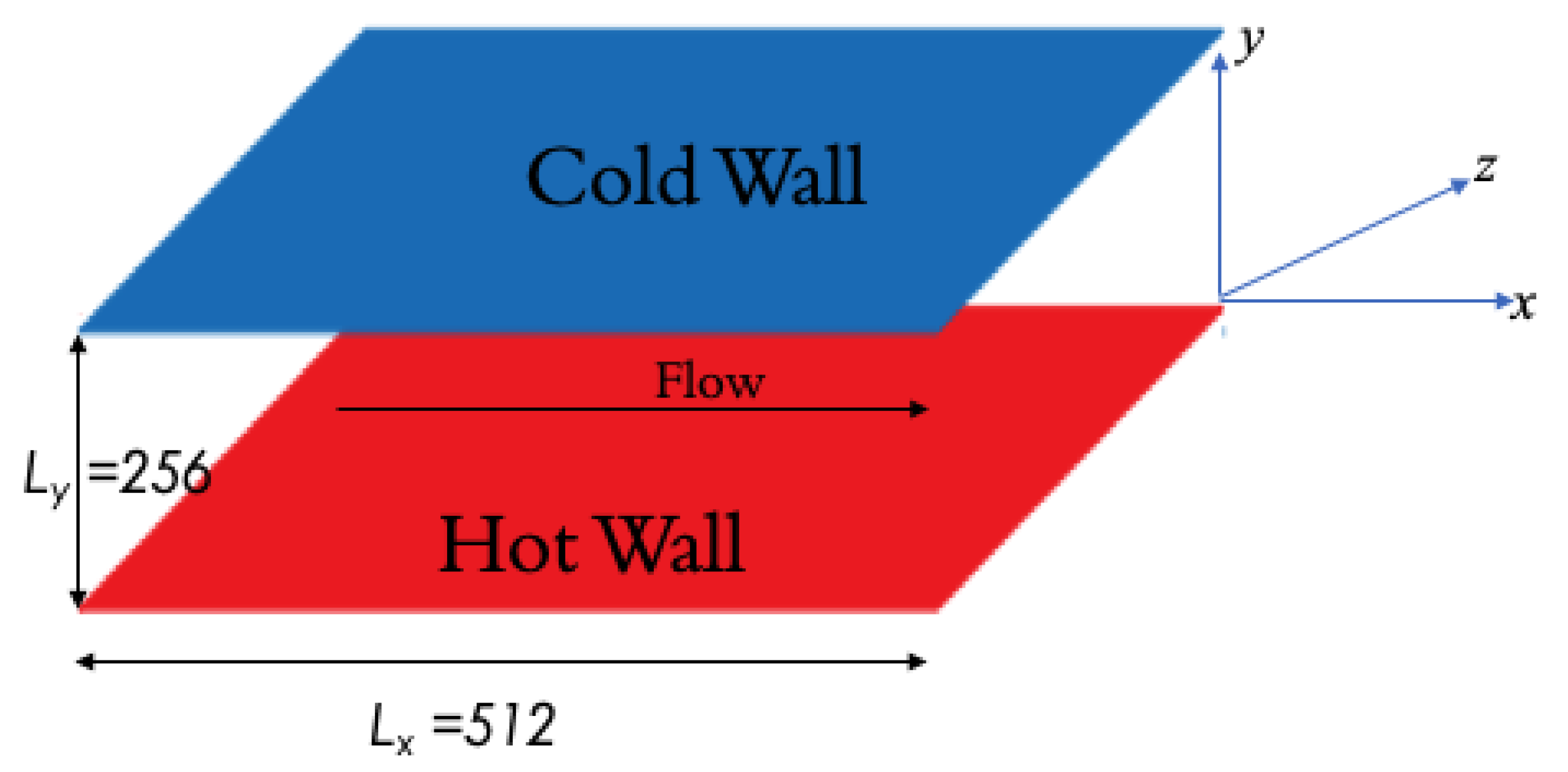
The channel flow configuration is used to study the mixed convection flow regime for liquid metal with a Prandtl number of 0.025. For fluids with a Prandtl number close to 1, the expected behavior of advected scalar turbulence is similar to the flow field, but the low Prandtl number case where the behavior of the flow and scalar field is expected to be quite different is chosen to analyze the flow and scalar field data separately. The top and the bottom walls of the channel are heated uniformly at a certain temperature. The cold wall is on the top with a lower temperature (), and the hot wall is on the bottom, and has a relatively higher temperature (). Flow enters the channel as shown in Figure 1 at a Reynolds number of , and the global Richardson number in the system is 0.1. Numerical simulation results of this problem were used to develop physical understanding, and then to develop a physics-based, reduced-order model. The DNS data were generated using Incompact-3d [26] (https://www.incompact3d.com) by considering the flow configuration in a horizontal channel discretized in grid points. A buoyancy force is induced throughout the flow field due to the temperature difference between the top wall and the bottom wall. The acceleration acts downward along the y direction because of gravity. The streamwise, wall-normal, and spanwise coordinates are represented by x, y, and z, respectively.
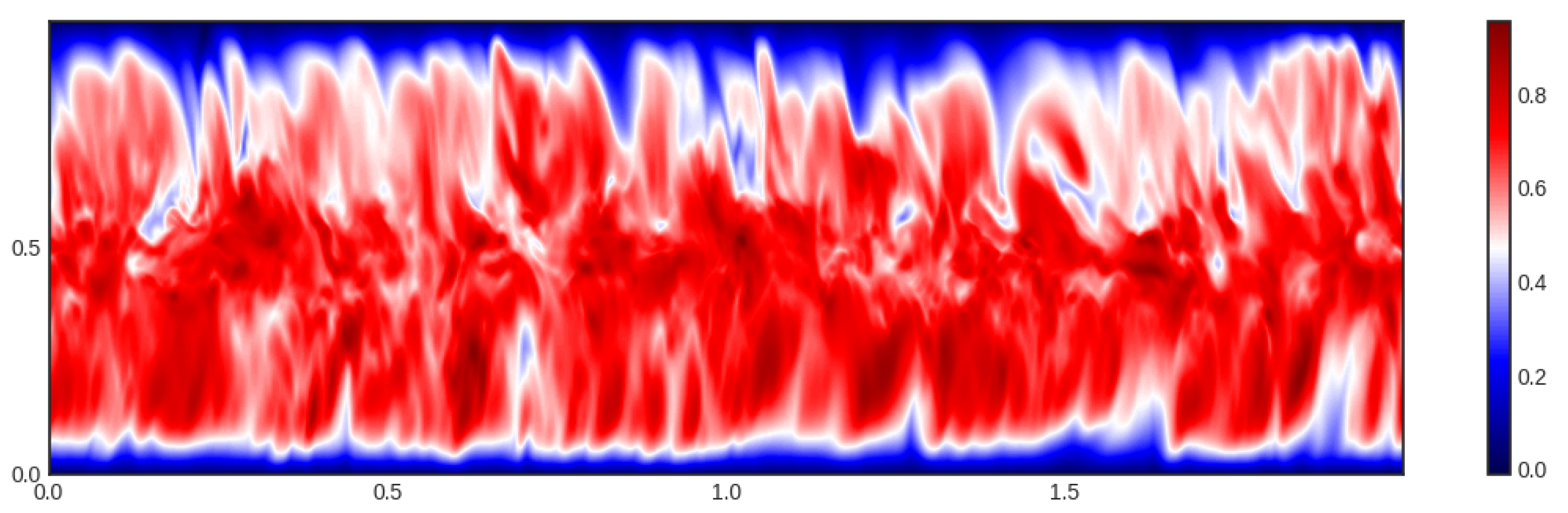
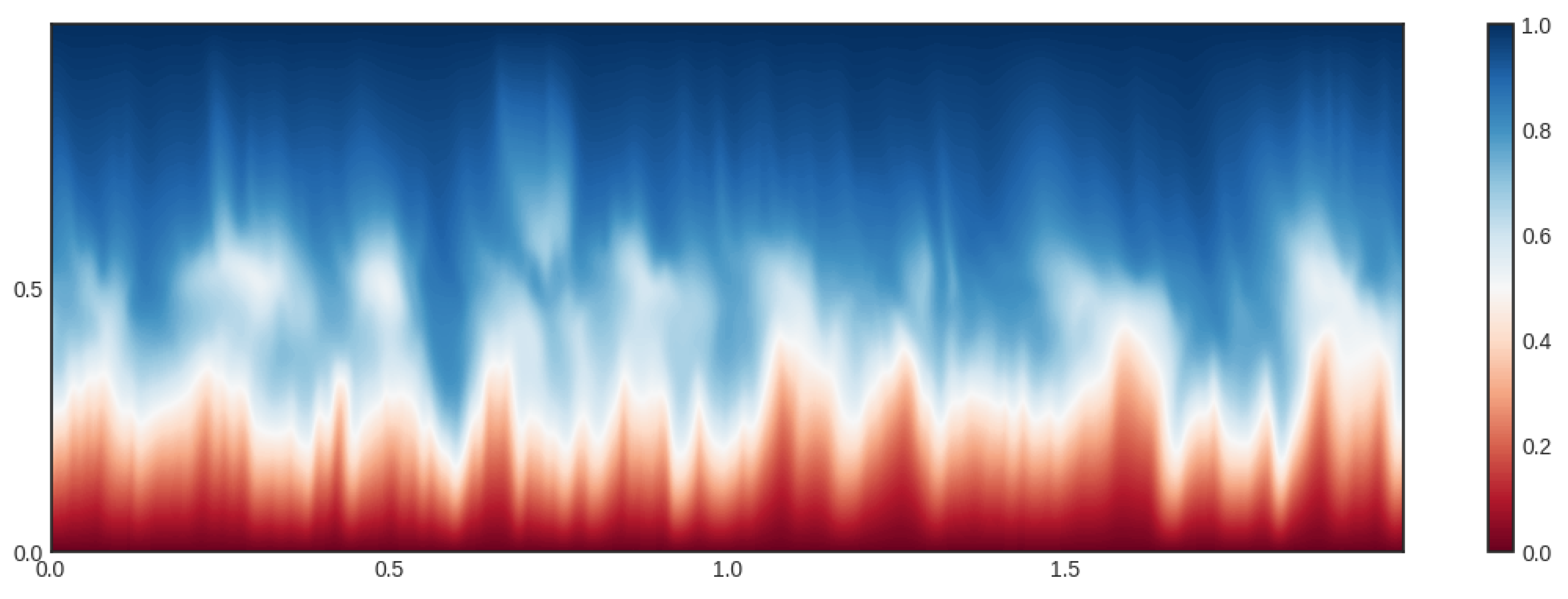
The 2D snapshots of the streamwise velocity field and temperature field at the Z-centerplane in the domain are presented in Figure 2 and Figure 3. In this flow configuration, the velocity and temperature signals were probed at the 128th grid point from the bottom hot plate.
Energy Cascading
The turbulent flow or convected scalar presented in this problem is expected to have multiple “hidden” and differentially correlated scales [5]. The interaction of these scales are highly localized in time. Based on this physical understanding of the turbulent fluctuations and the energy scales, the macroscopic behavior of the system is affected by the microscopic phenomena.
The interaction between the scales can be rigorously analyzed by computing probability density functions (PDF) of velocity or scalar fluctuations at different scales. The generic description of the energy cascading or interaction between different scales can be constructed by computing the transition or conditional PDF (cPDF) from the joint PDF (jPDF) at multiple scales. In other words, in order to reproduce the energy spectra of the original signal, multipoint cPDF must be generated, which is a cumbersome process and will not solve the intent of reduced-order emulation of the physical phenomenon. Coarse graining of dynamics can be done by approximating the system via a Markov process. Previous studies [27,28,29] have shown that this is a good enough approximation for turbulent jets, wall-bounded flows, and scalar turbulence. This allows the multipoint cPDF to be simplified to the cPDF computed from the probability of a new state jump from the most recent state which is, by definition, a Markovian process. By removing the length/time scale corresponding to memory, it is possible to approximate the process via a Markov model, and it was shown previously with the experimental data [27] that this length scale corresponds to the Taylor microscale. For jumps greater than this length scale, the condition of “Markovianity” will remain satisfied.
Moreover, owing to the very short time-scales associated with microscopic phenomena, it is often prohibitive to resolve them computationally or measure them experimentally. Therefore, this physics-based approach preserves the mesoscopic scale turbulent fluctuations as compared to traditional homogenization approaches.
3. Theory–Statistics-Based Projection
In this section, the development of the Markovian emulator from the data and the theoretical background to solve an inverse problem is discussed. Previously, several statistical mechanics interpretive models or closure models for turbulence were proposed by researchers (see references [7,29,30]). Pope et al. [30] proposed a linear Markov model for scalar turbulence based on grid turbulence experiments [30,31]. The simple mathematical description of the Markovian dynamics process in the continuous time framework can be described by an Ito semi-martingale.
A more generic, non-linear, statistical mechanics-based continuous time model can be derived using “Kramers–Moyal expansion” [32,33]. The validity of the Markovian assumption beyond the Taylor microscale was established by the researchers [27]. The non-linearity in the model comes from the higher-order dependence of the coefficients of the Langevin equation on the variable under consideration. This means the parameters of the model evolve in time. Very generically, a non-linear Langevin equation can be written for a generic variable “y”, which can take any specific form–velocity, temperature fluctuations, and so forth.
The coefficients and can be obtained from the first two terms of the Kramers–Moyal (KM) expansion. The KM expansion terms for the transition of probability current can be derived by starting from the definitions of the cPDF identity [32].
and substituting the Taylor series expansion of the “” function
The probability current can be expressed in terms of state transition probability or cPDF, as
which can be simplified to
Dividing by and setting the limit to 0 results in
Defining and substituting
leads to
The Kramers–Moyal (KM) expansion as derived is a generic result, where coefficients of each term can be expressed in terms of the respective moments:
If the Kramers–Moyal expansion stops at the second term, then it results in the Fokker–Planck equation
and the coefficients and can be obtained and substituted to form the Langevin equation (Equation (1)). If the process is Markovian, then the higher terms should go to zero, which is an important result from Pawula’s theorem, and allows the use of the first two terms to compute the coefficients of the Langevin equation (Equation (1)).
Equivalence to the Advection–Diffusion Equation
Classically, the dynamics of the scalar field is described by the advection–diffusion equation (see Equation (14)), which is a second-order partial differential equation. Temperature is a scalar, which can be defined in terms of entropy, where entropy is a measure of randomness accounting the number of microstates occupied by the system [34]. A stochastic analog for the microstates can be described as a non-linear Langevin equation (Equation (1)). Therefore, the advection–diffusion equation represents the dynamics of the probability density function of the occupied microstates. In its most generic form, the advection–diffusion equation can be written as the Fokker–Planck equation, a PDE which governs the evolution of PDF through the domain (see Equation (14)):
Equivalence between the Fokker–Planck and advection–diffusion equations can be demonstrated. The advective flux is driven by the “drift” component, , equivalent to the velocity variable in the advection–diffusion equation. Similarly, the diffusive component, , in the Fokker–Planck equation is analogous to the thermal diffusion attributed to local “molecular interactions” or “turbulent eddies”.
Since the physical dynamics are very important for building a statistical emulator of scalar or flow fluctuations, certain aspects and justifications for building these models are derived from the classical K-41 theory and Taylor’s hypothesis of local isotropy and frozen turbulence. Kolmogorov’s K-41 theory relies on the idea that the anisotropy introduced at production scales is gradually lost as energy is transferred to smaller scales. As a consequence, when the Reynolds number is sufficiently high, the smaller scales are independent of the production mechanisms, being locally isotropic and universal. Here, the small-scale isotropy is the property of velocity increments [5]. Local isotropy also means that flow is invariant from the rotational perspective.
Under Taylor’s frozen turbulence hypothesis, spatial measurements of fluctuations are possible from a single probe’s measurements [35] (applicable if the mean flow velocity is much larger than the fluctuating velocity). Owing to this, the spatial correlations can be approximated via the temporal correlations. In other words, the Taylor hypothesis assumes a statistical stationarity—that is, space translation will not change the measurement. Thus, it can be concluded that the temporal response at a fixed point in space can be viewed as the result of an unchanging spatial pattern convecting uniformly past the point [36]. Under these hypotheses, it is possible to build simple statistical models for small increments, as they are locally isotropic and stationary.
4. Results and Discussion
The velocity and temperature signals were obtained from the 128th grid point from the bottom hot plate in the mid-Z plane (as discussed in the physical domain description). These signal data are used to obtain the jPDF and cPDF, which are then used to compute the first and second diffusion coefficients by estimating moments.
4.1. Data Learning: Estimating Moments
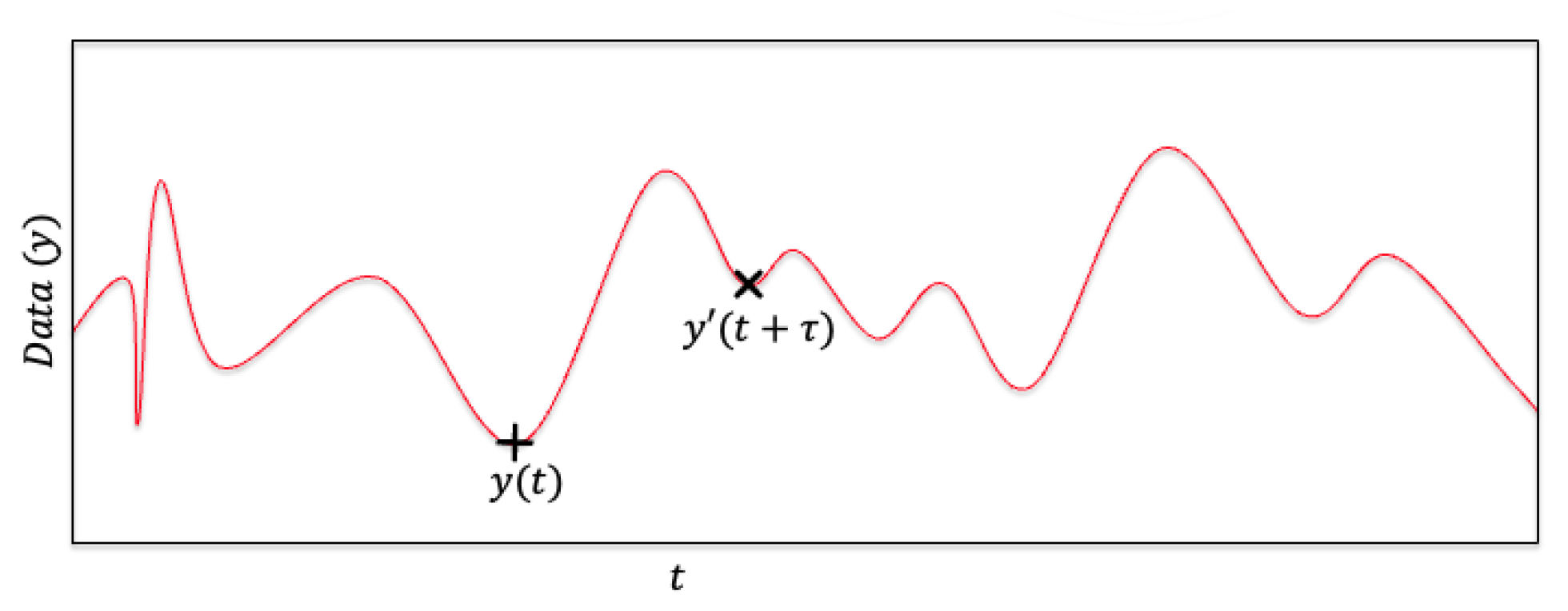
The joint probability can be computed via a shifted copy of the signal itself. This shift in the signal is generated via binning the data and counting the next state achieved by the signal for each fixed state for the subsequent higher .
The jPDF can be obtained for different values, and the Equation (12) shows that one of the key data-generated inputs of this method is the conditional probability, , which is required to compute the conditional moments of the data. This can be computed by making a vertical (or horizontal) cut in the joint probability distribution function see (Figure 4).
Once the conditional probability is obtained, then the conditional moments were evaluated, and the limiting value of the moments were computed by extrapolating the moments to . These conditional moments were evaluated for all the binning points of the series for varying lags (). Then, a simple regression of computed moments versus the binning points show the dependence of drift and diffusion coefficients with the measured signal span itself.
Two important pre-processing conditions which were evaluated before implementation of this model were that the data or time-series used for analysis were stationary and Markovian. It was shown in previous studies [27,33] that the Taylor microscale is the minimum length above which the turbulence shows memoryless behavior, since at that point, inertial length scales start and the cascade is known to show memoryless behavior. In other words, the smallest scales used for pre-processing should be above the Taylor microscale. The time-series used for computing conditional moments was obtained by subtracting the data from the time-shifted signal where the shifting time-scale, , was larger than the Taylor microscale, which was computed using the osculating parabola method from the autocorrelation of raw data. This ensures that the data used is Markovian and stationary.
The post-processing checks for the successful implementation of the Langevin model include how the PDF obtained from the Langevin model should compare well with the data, and the higher-order moments (n > 2) of the data, especially the fourth moment, is relatively small compared to the second moment. This then ensures that the Kramers–Moyal expansion stops at the second term and results in the Fokker–Planck equation or the equivalent advection–diffusion equation.
4.2. Velocity Data and Surrogate
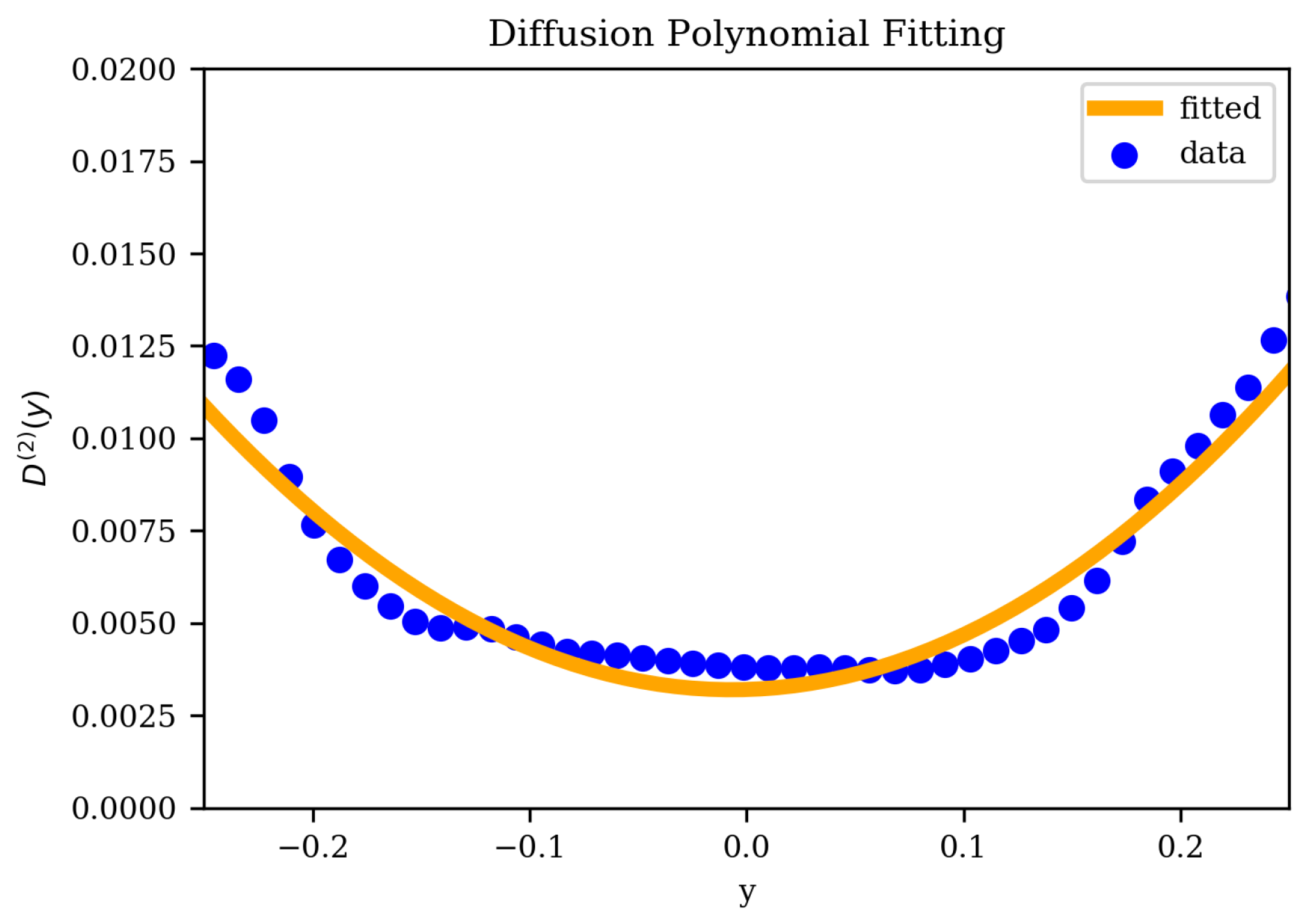
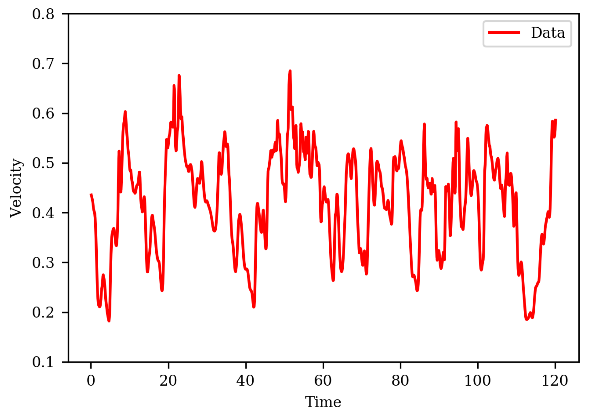
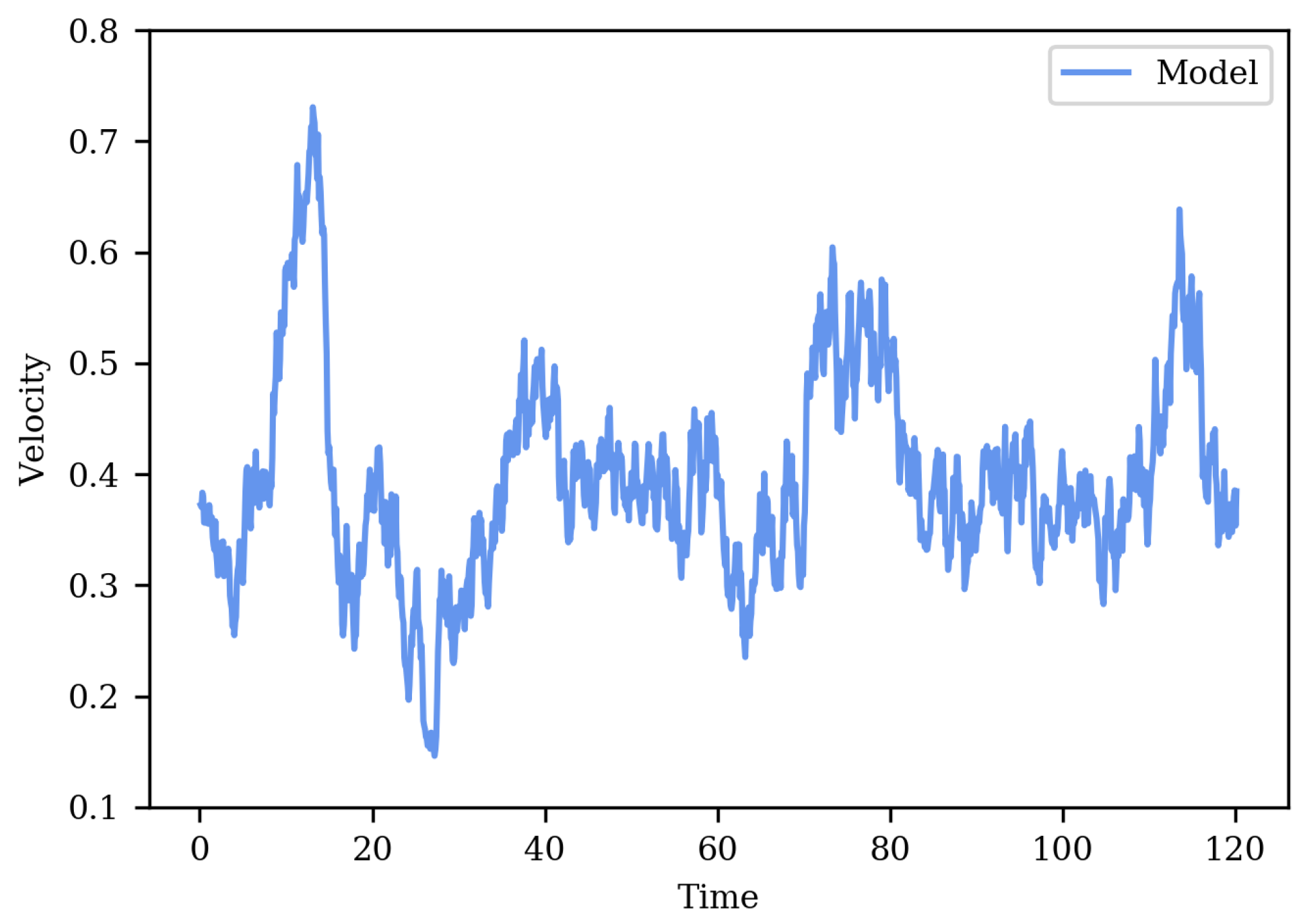
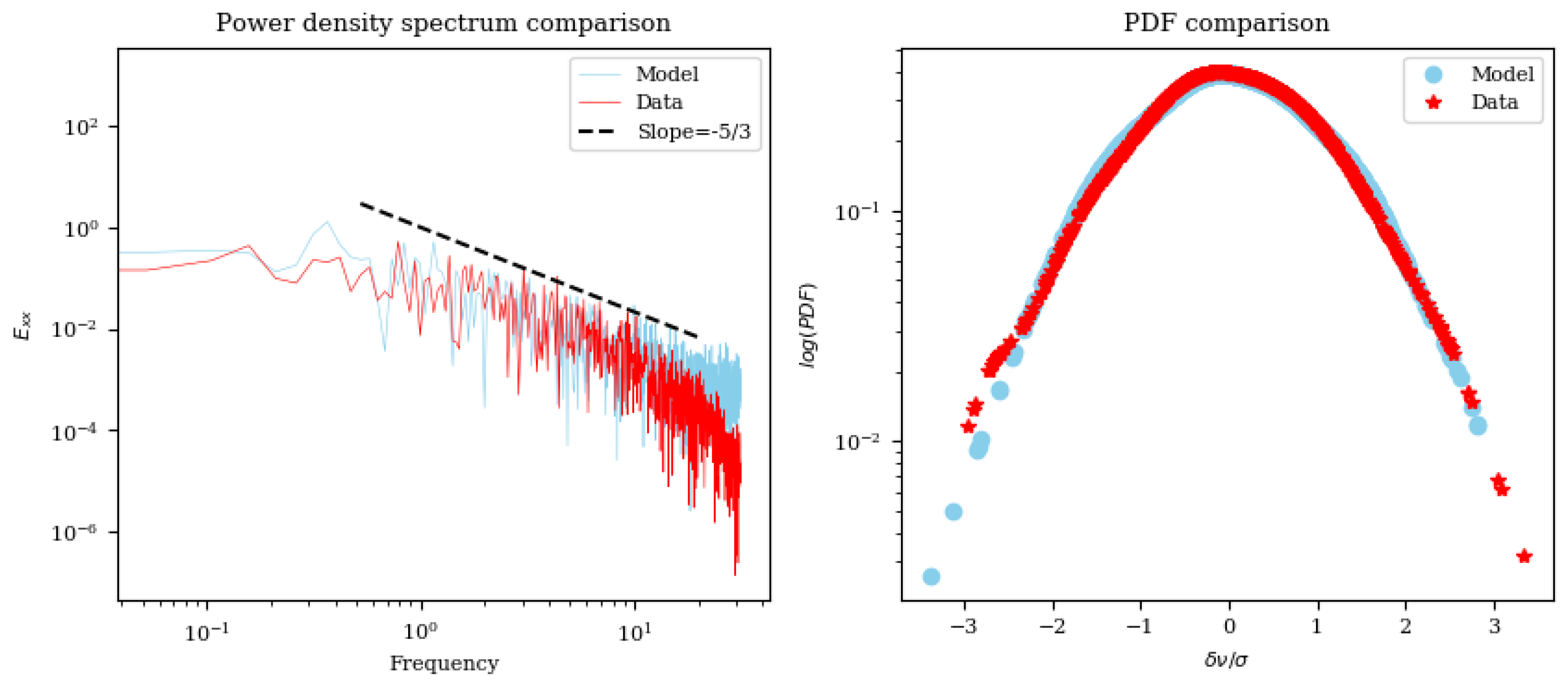
The first moment () tends to follow a linear trend with the velocity fluctuations, while the second moment () shows a quadratic trend. Figure 5 shows the example of the drift coefficient () calculated from a raw velocity time-series, along with the same data fitted to a first-order polynomial. Figure 6 shows an example of the diffusion coefficient () calculated from a raw velocity time-series, along with the same data fitted to a first-order polynomial. The fitted coefficients are then inserted back into the Langevin equation (Equation (1)) for velocity, and this equation is then integrated using the Euler–Maruyama method. The solution recovers the regenerated signal, which is then compared with the actual data (see Figure 7 and Figure 8). There are three comparative analyses used to examine the model—temporal evolution of the regenerated signal, Power Spectral Density (PSD), and PDF of fluctuations. It can be seen from the the results that the non-linear Langevin model developed by projecting DNS velocity data on KM expansion emulates the turbulent flow signal. The regenerated time-series from the Langevin model looks similar to the time-series obtained from DNS simulations. The PSD comparison shows that the model captures the expected −5/3 slope in the inertial regime (see Figure 9). At higher frequencies, the PSD of the model slightly deviates from the data, which is expected as the raw time-series was pre-processed to remove scales smaller than Taylor micro-scale for building conditional moments in the KM expansion. The Kramers–Moyal expansion is a Markovian model, so it will not be able to perfectly capture non-Markovian processes which are beyond Taylor’s micro-scale. The expansion ends at the second term, which is confirmed by the magnitude of the fourth coefficient being negligible as compared to the second term, thus satisfying Pawula’s theorem. The PDF comparison shows that the scale of fluctuations obtained from DNS data and the Langevin model are very similar.
4.3. Temperature Data and Surrogate
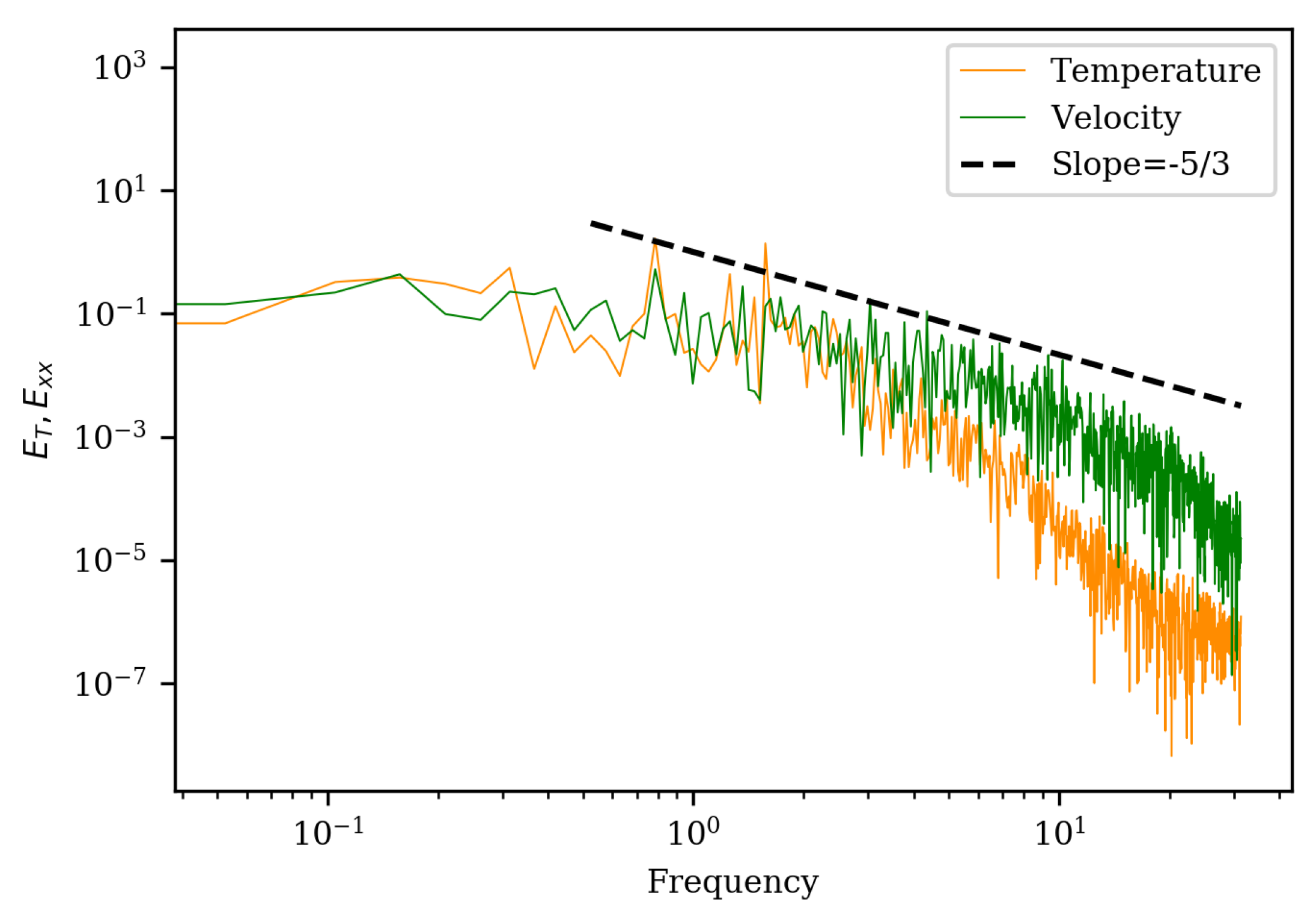
Some interesting differences are observed between the velocity and temperature time-series. The temperature data at the same location shows long-term memory effects, which can be attributed to the thermal diffusivity of the liquid metal. This point can be seen by drawing a PSD comparison (see Figure 10) of the probed velocity and temperature time-series. The PSD clearly shows the rapidly dropping energy cascade section in the temperature spectrum, with a slope of in the inertial regime, which is incongruent with the liquid metal behavior reported in the literature [37,38,39]. Beyond the expected inertial regime, the model is not expected to behave well, due to the high Prandtl number and high thermal diffusivity of the domain.
The temperature data were then used to construct a statistical surrogate in a manner similar to the velocity data. Following a similar process, the temperature signal from the DNS simulations was analyzed and projected on the KM expansion. Conditional moments and diffusion coefficients obtained show that higher coefficients can be neglected, as in the velocity case, resulting in retention of only the first two terms of KM expansion and leading to the Fokker–Planck equation, which is a generic mathematical representative to the advection–diffusion equation. Thus, the theoretically well-known governing equation for the scalar transport is conserved from the data.
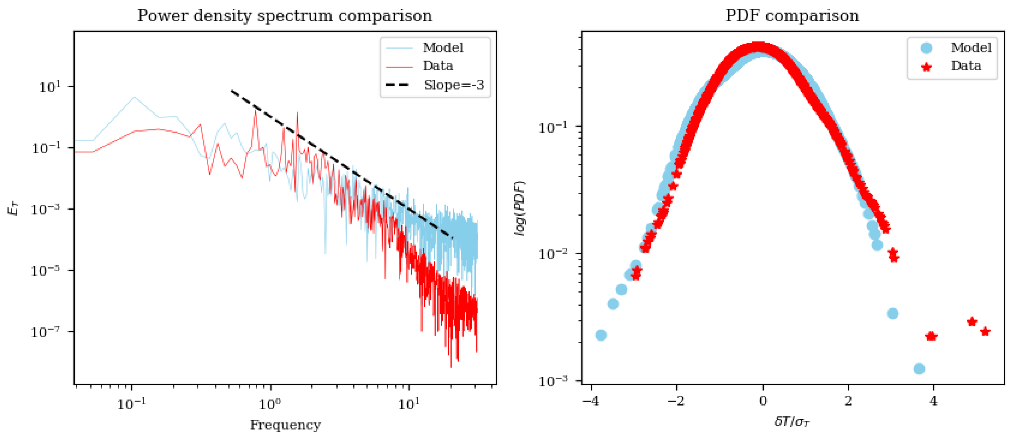
The Langevin model obtained from the conditional moments is then used to regenerate the signal. The comparison between the data and model is demonstrated in Figure 11. The model matches with the data in the inertial regime quite well by tracking the slope, which is a special case for liquid metals. Additionally, as expected, the PSD of the model time-series is expected to deviate from the data at higher frequencies due to high thermal diffusivity behavior and long-term memory effects. The PDF of the temperature fluctuations in the regenerated signal and the data show good agreement, demonstrating that the inverse problem, that is, the Langevin equation is successfully constructed.
5. Conclusions
This study introduced an alternative approach to overcome uncertainties arising from the limitations of simplified models in safety analysis tools without significantly increasing the computational costs. The high-resolution experiments or simulations of a certain sensitive component or subsystem, which are governed by highly nonlinear thermal physics, can be used to train the system. The work presented in this paper involved building a simple statistical reduced-order model or an emulator for the lost degrees of freedom by learning the parameters directly from the carefully accumulated data, either by running a model which describes the full dynamics of the equation or carefully collecting the data via controlled experiments. The statistical mechanics principles were adopted to build a Markovian model for the lost behavior attributed to filtering/averaging and projection of dynamics. This has been implemented and demonstrated on a canonical problem of liquid metal channel flow with differentially heated walls. A simple statistical surrogate, the Langevin equation, was constructed by probing the velocity and temperature signals in the DNS dataset of the liquid metal. The drift and diffusion coefficients of the Langevin equation were obtained with the help of the Kramers–Moyal expansion, capturing the Markovian processes. The statistical emulator was able to capture the essential details of the turbulent signal, and shows good statistical agreement with the raw DNS fluctuations. Some interesting differences between the velocity and temperature time-series at the same time-scales were shown. However, future work will need improvement of these emulators to capture the memory effects, that is, non-Markovian processes.
The local or microscopic behavior of the system can be studied using high-fidelity DNS or LES simulations, and then can be propagated to the system-level through an interface between the 1D and 3D codes. This can be done by studying the specific stochastic process driving the system by analyzing the time signals (velocity or temperature) using an unsupervised learning methodology introduced in the context of non-equilibrium statistical mechanics. These statistical emulators can be used to build closures for the 1D models, or can be used to provide the coupling mechanism. Stochastic surrogate representation can also be used in the correct depiction of inlet disturbances as an input for turbulent flow LES/DNS simulations. In cases of reactor scale geometries, future work is recommended to simulate reactor plena or geometries with complex flow behavior using LES models or experiments. The scalar turbulence statistics from these simulations can then be used to develop emulators for stochastic forcing or stochastic closures in 1D models. These modified 1D models with stochastic emulators might be the most efficient and accurate option to capture thermal stratification and local scalar mixing in reactor plena. These models can significantly improve the safety analysis and safety envelope calculations.
Author Contributions
M.R.—Algorithm and problem solving, plotting; H.B.—Writing and Editing. All authors have read and agreed to the published version of the manuscript.
Funding
This research was partly supported by DOE Nuclear Energy University Programs, and first author acknowledges the support of Nuclear Regulatory Commission fellowships.
Institutional Review Board Statement
Not applicable.
Informed Consent Statement
Not applicable.
Data Availability Statement
Available upon request.
Conflicts of Interest
The authors declare no conflict of interest.
References
- Gould, D.; Franken, D.; Bindra, H.; Kawaji, M. Transition from molecular diffusion to natural circulation mode air-ingress in high temperature helium loop. Ann. Nucl. Energy 2017, 107, 103–109. [Google Scholar] [CrossRef] [Green Version]
- Franken, D.; Gould, D.; Jain, P.K.; Bindra, H. Numerical study of air ingress transition to natural circulation in a high temperature helium loop. Ann. Nucl. Energy 2018, 111, 371–378. [Google Scholar] [CrossRef]
- Ward, B.; Clark, J.; Bindra, H. Thermal stratification in liquid metal pools under influence of penetrating colder jets. Exp. Therm. Fluid Sci. 2019, 103, 118–125. [Google Scholar] [CrossRef]
- Ward, B.; Wiley, A.; Wilson, G.; Bindra, H. Scaling of thermal stratification or mixing in outlet plena of SFRs. Ann. Nucl. Energy 2018, 112, 431–438. [Google Scholar] [CrossRef]
- Frisch, U.; Kolmogorov, A.N. Turbulence: The Legacy of AN Kolmogorov; Cambridge University Press: Cambridge, UK, 1995. [Google Scholar]
- Sreenivasan, K.R. Turbulent mixing: A perspective. Proc. Natl. Acad. Sci. USA 2018, 116, 18175–18183. [Google Scholar] [CrossRef] [PubMed] [Green Version]
- Durbin, P. A stochastic model of two-particle dispersion and concentration fluctuations in homogeneous turbulence. J. Fluid Mech. 1980, 100, 279–302. [Google Scholar] [CrossRef]
- Taylor, G.I. Diffusion by continuous movements. Proc. Lond. Math. Soc. 1922, 2, 196–212. [Google Scholar] [CrossRef]
- Osborne, D.; Vassilicos, J.; Sung, K.; Haigh, J. Fundamentals of pair diffusion in kinematic simulations of turbulence. Phys. Rev. E 2006, 74, 036309. [Google Scholar] [CrossRef] [Green Version]
- Jullien, M.C.; Paret, J.; Tabeling, P. Richardson pair dispersion in two-dimensional turbulence. Phys. Rev. Lett. 1999, 82, 2872. [Google Scholar] [CrossRef] [Green Version]
- Roberts, P.J.; Webster, D.R. Turbulent Diffusion; ASCE Press: Reston, VA, USA, 2002. [Google Scholar]
- Obabko, A.; Fischer, P.; Marin, O.; Merzari, E.; Pointer, D. Verification and Validation of Nek5000; NURETH-16; Thermal Hydraulics: Chicago, IL, USA, 2015. [Google Scholar]
- Thomas, J.; Fanning, T.; Vilim, R.; Briggs, L. Validation of the Integration of CFD and SAS4A/SASSYS-1: Analysis of EBR-II Shutdown Heat Removal Test 17; American Nuclear Society: La Grange Park, IL, USA, 2012; Volume 1, pp. 692–700. [Google Scholar]
- Huber, K.; Fanning, T.H.; Thomas, J.W. Coupled calculations of SAS4A/SASSYS-1 and STAR-CCM+ for the SHRT-45R test in EBR-II. In Proceedings of the 16th International Meeting on Nuclear Reactor Thermal Hydraulics NURETH-16, Chicago, IL, USA, 30 August–4 September 2015. [Google Scholar]
- Baviere, R.; Tauveron, N.; Perdu, F.; Garre, E.; Li, S. A first system/CFD coupled simulation of a complete nuclear reactor transient using CATHARE2 and TRIO_U. Preliminary validation on the Phenix Reactor Natural Circulation Test. Nucl. Eng. Des. 2014, 277, 124–137. [Google Scholar] [CrossRef]
- Hu, R.; Zhu, Y.; Kraus, A. Advanced Model Developments in SAM for Thermal Stratification Analysis during Reactor Transients; Technical Report; Argonne National Lab.: Lemont, IL, USA, 2018. [Google Scholar]
- Wang, C.; Wu, X.; Kozlowski, T. Surrogate-Based Inverse Uncertainty Quantification of TRACE Physical Model Parameters Using Steady-State PSBT Void Fraction Data. In Proceedings of the 17th International Topical Meeting on Nuclear Reactor Thermal Hydraulics (NURETH 17), Xi’an, China, 3–8 September 2017; pp. 3–8. [Google Scholar]
- Huang, D.; Abdel-Khalik, H.; Rabiti, C.; Gleicher, F. Dimensionality reducibility for multi-physics reduced order modeling. Ann. Nucl. Energy 2017, 110, 526–540. [Google Scholar] [CrossRef]
- Wu, X.; Kozlowski, T. Inverse uncertainty quantification of reactor simulations under the Bayesian framework using surrogate models constructed by polynomial chaos expansion. Nucl. Eng. Des. 2017, 313, 29–52. [Google Scholar] [CrossRef]
- Bindra, H.; Uddin, R. Effects of modeling assumptions on the stability domain of BWRs. Ann. Nucl. Energy 2014, 67, 13–20. [Google Scholar] [CrossRef]
- Liu, Y.; Dinh, N. Validation and Uncertainty Quantification for Wall Boiling Closure Relations in Multiphase-CFD Solver. Nucl. Sci. Eng. 2019, 193, 81–99. [Google Scholar] [CrossRef] [Green Version]
- Batchelor, G. Diffusion in a field of homogeneous turbulence: II. The relative motion of particles. Math. Proc. Camb. Philos. Soc. 1952, 48, 345–362. [Google Scholar] [CrossRef]
- Klir, G.J.; Yuan, B. Fuzzy Sets and Fuzzy Logic: Theory and Applications; Prentice Hall PTR New Jersey: Englewood Cliffs, NJ, USA, 1995; Volume 574. [Google Scholar]
- Booker, J.; Ross, T. An evolution of uncertainty assessment and quantification. Sci. Iran. 2011, 18, 669–676. [Google Scholar] [CrossRef] [Green Version]
- Gairola, A.; Bindra, H. Lattice Boltzmann method for solving non-equilibrium radiative transport problems. Ann. Nucl. Energy 2017, 99, 151–156. [Google Scholar] [CrossRef] [Green Version]
- Laizet, S.; Lamballais, E. High-order compact schemes for incompressible flows: A simple and efficient method with quasi-spectral accuracy. J. Comput. Phys. 2009, 228, 5989–6015. [Google Scholar] [CrossRef]
- Renner, C.; Peinke, J.; Friedrich, R. Experimental indications for Markov properties of small-scale turbulence. J. Fluid Mech. 2001, 433, 383–409. [Google Scholar] [CrossRef]
- Tutkun, M. Markovian properties of velocity increments in boundary layer turbulence. Phys. D Nonlinear Phenom. 2017, 351, 53–61. [Google Scholar] [CrossRef]
- Peinke, J.; Tabar, M.R.; Wachter, M. The Fokker–Planck approach to complex spatiotemporal disordered systems. Annu. Rev. Condens. Matter Phys. 2019, 10, 107–132. [Google Scholar] [CrossRef]
- Pope, S.B. Simple models of turbulent flows. Phys. Fluids 2011, 23, 011301. [Google Scholar] [CrossRef]
- Warhaft, Z. The interference of thermal fields from line sources in grid turbulence. J. Fluid Mech. 1984, 144, 363–387. [Google Scholar] [CrossRef]
- Risken, H. Fokker-planck equation. In The Fokker-Planck Equation; Springer: Berlin/Heidelberg, Germany, 1996; pp. 63–95. [Google Scholar]
- Friedrich, R.; Peinke, J. Description of a turbulent cascade by a Fokker-Planck equation. Phys. Rev. Lett. 1997, 78, 863. [Google Scholar] [CrossRef]
- Reif, F. Fundamentals of Statistical and Thermal Physics; Waveland Press: Long Grove, IL, USA, 2009. [Google Scholar]
- Pope, S.B. Turbulent Flows; Cambridge University Press: Cambridge, UK, 2000. [Google Scholar]
- Moin, P. Revisiting Taylor’s hypothesis. J. Fluid Mech. 2009, 640, 1–4. [Google Scholar] [CrossRef] [Green Version]
- Gibson, C.H. Zero gradient points in turbulent mixing. In Structure and Mechanisms of Turbulence II; Springer: Berlin/Heidelberg, Germany, 1978; pp. 347–352. [Google Scholar]
- Cioni, S.; Ciliberto, S.; Sommeria, J. Temperature structure functions in turbulent convection at low Prandtl number. EPL Europhys. Lett. 1995, 32, 413. [Google Scholar] [CrossRef]
- Clay, J.P. Turbulent Mixing of Temperature in Water, Air and Mercury. Ph.D. Thesis, University of California, San Diego, CA, USA, 1974. [Google Scholar]
Figure 1.
Simulation domain grid points.

Figure 2.
Two-dimensional (2D) snapshot of the streamwise velocity field along the Z-center plane.

Figure 3.
2D snapshot of the temperature field along the Z-center plane.

Figure 4.
Methodology to obtain conditional probability from the time-series data.

Figure 5.
Drift parameter fitted to a first-order polynomial.

Figure 6.
Diffusion parameter fitted to a second-order polynomial.

Figure 7.
Raw velocity data from the probe.

Figure 8.
Regenerated velocity obtained from the Langevin model.

Figure 9.
Power Spectral Density (PSD) and probability density functions (PDF) comparison of the velocity fluctuations obtained from direct numerical simulations (DNS) data and model solution.
Figure 9.
Power Spectral Density (PSD) and probability density functions (PDF) comparison of the velocity fluctuations obtained from direct numerical simulations (DNS) data and model solution.

Figure 10.
Spectrum of velocity and temperature data showing a significant difference in the scalar turbulence in liquid metal flow.
Figure 10.
Spectrum of velocity and temperature data showing a significant difference in the scalar turbulence in liquid metal flow.

Figure 11.
PSD and PDF comparison of the temperature fluctuations obtained from DNS data and model solution.
Figure 11.
PSD and PDF comparison of the temperature fluctuations obtained from DNS data and model solution.

Publisher’s Note: MDPI stays neutral with regard to jurisdictional claims in published maps and institutional affiliations. |
© 2021 by the authors. Licensee MDPI, Basel, Switzerland. This article is an open access article distributed under the terms and conditions of the Creative Commons Attribution (CC BY) license (http://creativecommons.org/licenses/by/4.0/).
Share and Cite
MDPI and ACS Style
Ross, M.; Bindra, H. Statistical Mechanics-Based Surrogates for Scalar Transport in Channel Flow. Fluids 2021, 6, 79. https://0-doi-org.brum.beds.ac.uk/10.3390/fluids6020079
AMA Style
Ross M, Bindra H. Statistical Mechanics-Based Surrogates for Scalar Transport in Channel Flow. Fluids. 2021; 6(2):79. https://0-doi-org.brum.beds.ac.uk/10.3390/fluids6020079
Chicago/Turabian StyleRoss, Molly, and Hitesh Bindra. 2021. "Statistical Mechanics-Based Surrogates for Scalar Transport in Channel Flow" Fluids 6, no. 2: 79. https://0-doi-org.brum.beds.ac.uk/10.3390/fluids6020079