
Hydrodynamics of Prey Capture and Transportation in Choanoflagellates


1
Department of Mechanical Engineering, Technical University of Denmark, DK-2800 Kgs. Lyngby, Denmark
2
National Institute of Aquatic Resources and Centre for Ocean Life, Technical University of Denmark, DK-2800 Kgs. Lyngby, Denmark
3
Computational Science and Engineering Laboratory, ETH, CH-8092 Zürich, Switzerland
*
Author to whom correspondence should be addressed.
Fluids 2021, 6(3), 94; https://0-doi-org.brum.beds.ac.uk/10.3390/fluids6030094
Submission received: 27 December 2020
/
Revised: 10 February 2021
/
Accepted: 13 February 2021
/
Published: 27 February 2021
(This article belongs to the Special Issue Ecological Fluid Dynamics)
Abstract
:Choanoflagellates are unicellular microscopic organisms that are believed to be the closest living relatives of animals. They prey on bacteria through the act of the continuous beating of their flagellum, which generates a current through a crown-like filter. Subsequently, the filter retains bacterial particles from the suspension. The mechanism by which the prey is retained and transported along the filter remains unknown. We report here on the hydrodynamic effects on the transportability of bacterial prey of finite size using computational fluid dynamics. Here, the loricate choanoflagellate Diaphaoneca grandis serves as the model organism. The lorica is a basket-like structure found in only some of the species of choanoflagellates. We find that although transportation does not entirely rely on hydrodynamic forces, such forces positively contribute to the transportation of prey along the collar filter. The aiding effects are most possible in non-loricate choanoflagellate species, as compared to loricate species. As hydrodynamic effects are strongly linked to the beat and shape of the flagellum, our results indicate an alternative mechanism for prey transportation, especially in biological systems where having an active transport mechanism is costly or not feasible. This suggests an additional potential role for flagella in addition to providing propulsion and generating feeding currents.
1. Introduction
Choanoflagellates are microscopic filter feeders that are known to be a major contributor to aquatic microbial foodwebs [1]. Their contribution is related to their ability to effectively feed on bacteria in sea water (usually in size [2]), and in return, they regenerate inorganic nutrients for the growth of unicellular algae [2]. In addition to their ecological importance, choanoflagellates are subjected to great interest due to their ancestral relationship with animals [3].
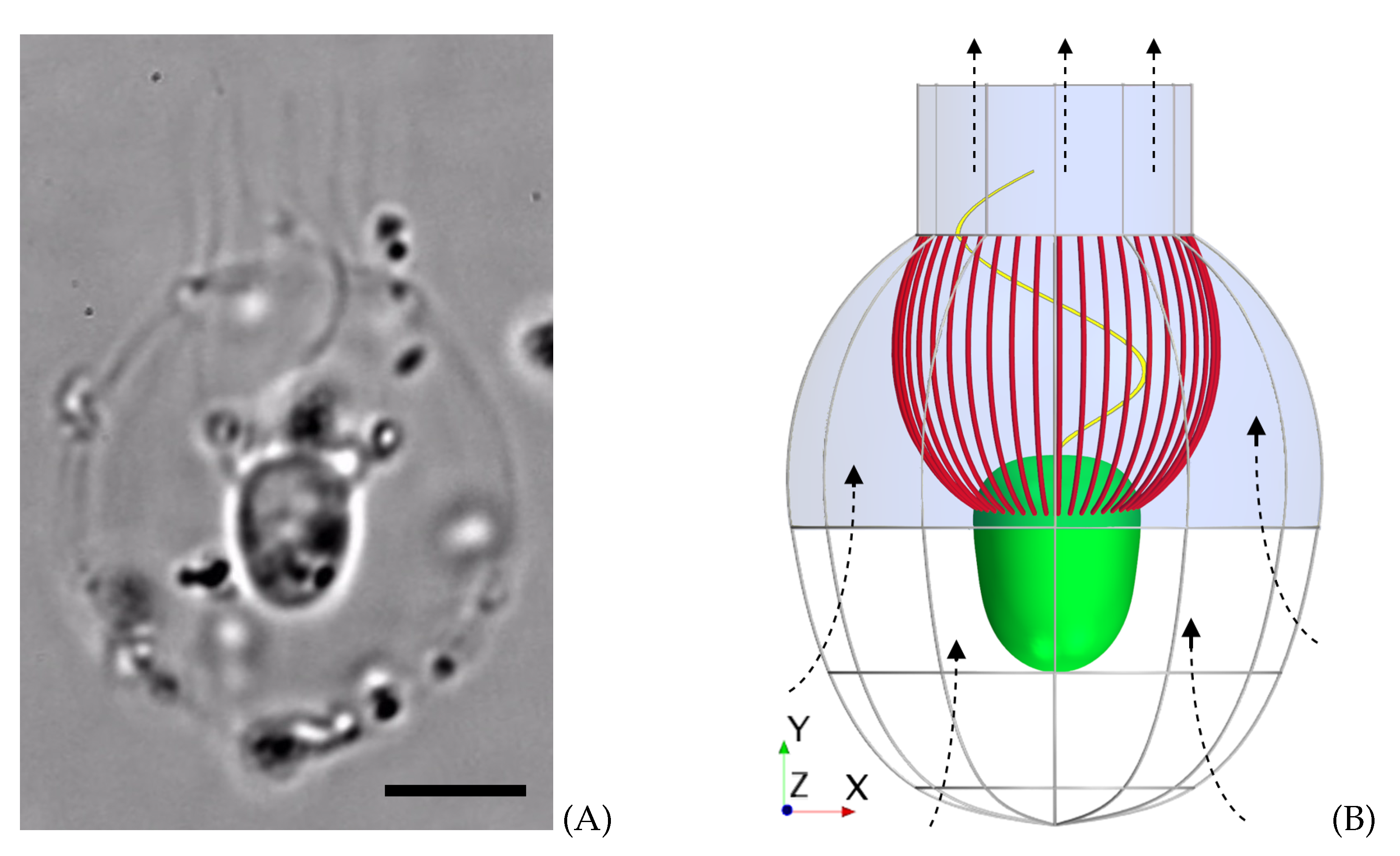
The choanoflagellate cell is characterized by a beating flagellum surrounded by a crown-like collar filter made up of a single layer of microvilli tentacles. Some choanoflagellate species also construct an extra-cellular structure, the lorica, a covering that consists of a two-layered arrangement of costae made up of rod-shaped costal strips. The lorica structure bears resemblance to a basket-like cage, from which the collar and cell are suspended [2]. All morphological characteristics are shown in Figure 1. The continuous beating of the flagellum acts as a pumping mechanism that draws water through the collar and, thus, retains appropriately sized bacteria [2]. Hydrodynamic characteristics are therefore crucial in understanding prey capture within these microscopic organisms. Due to the low concentration of prey particles in the suspension, choanoflagellates must clear a volume of water equivalent to about one million times that of their own body daily [4]. Previously, the flow-inducing flagellum was believed to take the shape of a thin bare rod. However, recently, it has been shown that such high clearance rates are only feasible if the flagellum is modeled as a thin wide sheet, representing a flagellar vane, oriented perpendicularly to the plane of beating [5]. The presence of a flagellar vane has been observed and explored in several species of choanoflagellates and choanocytes [6,7], but it remains unknown if a vane is present in all species. Similarities in the collar–flagellum system between choanoflagellates and choanocytes in sponges have led to the belief that their collar–flagellum interactions have both evolved in aspiration to optimize fluid flow through micro-scale filters [6].
The near-cell feeding flow in choanoflagellates still remains poorly understood due to simplified computational analyses and a lack of quantitative experimental results [2,8]. However, the recent discovery showing the necessity of a sheet-like flagellum structure has improved our understanding of the near-cell feeding flow, and thereby allows us to model it more accurately [5,7]. This new flagellum model was recently utilized in a study focused on the hydrodynamic functionality of the lorica [9]. Because not all choanoflagellates construct the lorica, the nature of its adaptive value has sparked curiosity. The study concluded that the lorica is not beneficial in terms of prey encounters [9]. Instead, the study argues, that the lorica enhances prey capture efficiency by improving the prey retention of the filter. Furthermore, the study considered the local velocity field between the filter openings in the flagellum beat plane, simulated both with and without the presence of the lorica. Here, a significant difference in the magnitude of the velocity field was found. In addition, the snapshots of the velocity fields ([9] Figure 9 therein) show that part of the flow field is directed both away from the collar and down towards the cell. These traits present a significant opportunity to understand the transportation process of prey, as the captured prey particles are directly influenced by the flow through the filter openings.
Many marine organisms (including unicellular ciliates/flagellates or multicellular organisms, such as copepods and starfish larvae) use an appendage to generate a feeding current, which facilitates the prey encounter process by bringing prey particles to their prey-capturing area. Furthermore, ciliary bands on the surface of starfish larvae facilitate transportation of the prey particles along the body toward the mouth [10]. Many protists, however, take advantages of surface motility by utilizing microtubule-filled extensions to capture and handle prey particles (cf. Bloodgood [11]). Bloodgood reviewed different examples of the surface motility in these protists, which always happens “on plasma membrane domains associated with microtubule cytoskeletons that vary greatly in complexity” [11]. Choanoflagellates, however, do not have these extensions, and it has been argued that prey transportation in choanoflagellates must have a different underlying mechanism [11]. The possibility that prey transportation in choanoflagellates relies on molecular motors, such as encasement in pseudopods, has previously been explored [12]. However, the observations did not support the presence of any molecular motors. Instead, it was hypothesized that the flow of water might contribute to the bacterial transport.
The present study will examine the hydrodynamic effects on bacterial transport using computational fluid dynamics (CFD). The study will utilize the loricate choanoflagellate Diaphanoeca grandis as the model morphology. Moreover, the hydrodynamic effects of the lorica will also be explored by studying an artificial non-loricate model of D. grandis. The analysis will consist of a static and a dynamic approach. The static approach endeavors to quantify the force contribution of the local flow on the bacterial surface. In theory, the prey are force and torque free when drifting freely within the flow, since any forces or torques felt by the prey are balanced by counteracting forces and torques due to the movement of the prey. The prey forces are attained by systematically fixing the prey along the collar surface, thus eliminating the motion and, hence, the counteracting forces and torques. The dynamic approach will allow the bacterial prey to move freely. Here, the effects on the flow caused by fixating the prey will be studied, as well as the correspondence between the static and dynamic results.
2. Methods
This section describes the methods utilized in the static and dynamic studies. The advantages and limitations of the solution procedures will be discussed, as well as the degree of accuracy that we credit to the numerical CFD model. Furthermore, we describe in detail which parameters are varied and to what extent.
2.1. Computational Fluid Dynamics
The flow characteristics of D. grandis were evaluated numerically using the commercial CFD software STAR-CCM+ (14.02.010-R8). Here, the computational domain was discretized using a combination of polyhedral and prism cells. Finite disjoint overset meshes discretized the ambient prey flow and secured connectivity with the remaining computational domain using linear interpolation. The governing equations were solved using the finite volume method.
The traveling wave that models the shape of the flagellum beat displacement is orientated relative to the coordinate system seen in Figure 1B and given by [9]:
Here, is the y-coordinate at the flagellum base (the position at which the cell and flagellum connect), is the characteristic length scale of the amplitude modulation, denotes the wave number, and the angular frequency. Lastly, gives the lateral displacement of the flagellum along the x-axis with respect to the longitudinal position from the flagellum base and a specific instant in time, t, within a beat cycle. The characteristic parameters in Equation (1) are given for the model organism D. grandis in Table 1.
2.1.1. Placement of Fixed Prey
When constructing the model morphology of D. grandis, the assumption of symmetry around the longitudinal center axis is utilized in shaping the lorica, filter, and cell. This allows for each part’s surface to be constructed as a simple curve, which can readily be revolved around the center axis of symmetry (Figure 2A). The equations for the curves of revolutions were obtained by averaging the outline of the mid-plane view of six different instances of the species [5,9]. The first resultant curvature equation models both the lorica dome, , and the cell, , and the second curvature equation models the collar filter, . Both curvature equations are given, respectively, as:
where , , , and are morphological parameters unique to the lorica and cell outline (Supplementary Information S8.1, Table S1), and and are the polar angles at which the filter meets the cell and lorica, respectively. The polar angle is defined relative to the longitudinal center axis, as seen in Figure 2A.
Forty-eight microvilli tentacles are distributed equally along the collar surface. The lorica dome and chimney are modeled as an impermeable baffle, where the ribs in the inferior part of the lorica (pictured in Figure 1B) are neglected for simplicity [9]. The flagellar vane is modeled as a wide sheet, which corresponds to the vane being slightly smaller than the diameter of the collar at the collar base. The traveling waveform of the beat of the flagellar vane is given in Equation (1), along with additional morphological and kinematic parameters for D. grandis (Table 1). The resulting CFD model morphology is pictured in Figure 2C. All surfaces (i.e., surfaces of the filter, the cell, the flagellum, and the lorica) are subject to the no-slip boundary condition.
The analysis will consider four different prey types: three spherical preys and one elongated prey (Table 2). The medium-sized prey, , will serve as the reference prey. The surface forces on each prey are recorded with respect to its local coordinate system. The local coordinate system is placed such that the x-axis is parallel to the normal vector at the point of prey–collar contact, and equivalently, the y-axis is parallel to the tangent vector. Using Equation (3), the gradients of the tangent, , and the normal vector, , are given by:
Furthermore, the local x-axis is directed towards the collar, and the local y-axis is directed away from the cell, as seen in Figure 2B.
The prey will be placed in two vertical perpendicular planes, each of which contains the longitudinal symmetry axis. In the first plane, called the beat plane (-plane in Figure 1), the prey will be placed on the right-hand side and left-hand side of the collar, denoted R and L, respectively. In the second plane, called the vane plane (-plane in Figure 1), the prey will similarly be placed on the back and front of the collar with respect to the view pictured in Figure 1. These two positions are denoted B and F, respectively. In each of the four positions, and the vertical position on the collar will be varied in three ways: at the bottom (), the middle (), and the top (), summing to a total of 12 positions. As an example, a medium-sized prey placed at the middle and on the left-hand side of the collar is referred to as: .
2.1.2. Governing Equations and Hydrodynamic Effects
For the prey particles captured by D. grandis, the Reynolds number () is in the order of . Here, is the fluid density, is the fluid dynamic viscosity, D is the characteristic length scale given by the diameter of the prey, and is the characteristic velocity of the flagellum, where and f denote the wavelength and frequency of the beating flagellum (cf. Supplementary Information S8.1). We note that a flow at this Reynolds number is governed by the time-independent Stokes equations:
where u and p denote the flow velocity and pressure, respectively. The time independency allows for the flow to be resolved in a series of discrete time steps, as the response of the fluid to the motion of boundaries can be considered instantaneous [13]. One flagellum beat cycle is discretized into 25 time steps. Doubling the number of time steps introduces a variation of less than 1% in the results [5]. Although it suffices to solve the Stokes equations, the full Navier–Stokes equations are solved at each discrete point in time by the CFD software. In combination with using mesh-morphing techniques, this allows for the flagellum position to be updated in each time step in a computationally efficient way. Given the symmetry of prey placed in the same plane but on opposing sides of the collar, it is only necessary to model half of a flagellum beat cycle. However, to ensure that mesh morphing does not have a significant impact on the symmetry at hand, we still choose to simulate the entire beat cycle.
An overset mesh using linear interpolation between the overset and background meshes is added around all prey particles, which allows for the same mesh to be used in both the dynamic and static simulations. The drawback of using an overset mesh in the static setting is that it is not possible for the body within the overset to be in direct contact with another surface. Subsequently, we introduce a gap between the prey and the microvilli. The combination of introducing a gap of size ∼5% of the prey radius and opting for the overset mesh method has been shown to result in an accumulated variation of up to ∼5% in the calculated prey forces as compared to a mesh without overset. Similarly to the mesh-morphing techniques used for updating the flagellum position, an overset mesh greatly reduces the solver workload in the dynamic prey simulations, as the regeneration of the entire volume mesh in each time step becomes dispensable.
The computational domain is discretized using from 6 to 11 million computational cells, where the highest density of cells is found along the microvilli tentacles and prey surfaces. This cell density is kept approximately constant for all analyses. The computational cost for a full simulation containing 11 million cells is approximately 50 h when performed on seven 16-core nodes (Xeon E5-2650 running at 2.60 GHz). The extent of the prey overset mesh is increased when the prey size is increased; hence, to obtain a sufficient connectivity between the two grids, the extent of refined cells in the background mesh has to increase accordingly. The mesh is pictured in Supplementary Information S8.3, Figure S3. In the loricate case using , the discretization error was shown to cause a variation of less than 1% in the measured prey forces and the time-averaged clearance rate through the filter (Supplementary S8.3). Here, a very fine mesh acted as an exact solution; thus, the discretization error was quantified based on a comparison with this solution. The geometry is contained within a spherical computational domain with a radius of , where a pressure boundary condition (B.C.) is applied to the outer surface (note the drawbacks of the pressure B.C. in Supplementary Information S8.2). Increasing the computational domain radius to results in a variation of less than in the results [5].
The hydrodynamic forces, F, and torque, L, acting on the fixed prey are obtained by integrating the stress tensor, , over the prey surface [13], S:
where the stress tensor is given by ( is the identity tensor), denotes the normal vector directed outwards from the prey surface, and denotes the position vector on the prey surface. Hence, prior to constructing the stress tensor, the pressure, p, and velocity, , of the incompressible fluid must be computed.
For a fixed sphere of radius r held in a uniform stream of velocity U, the Stokes law states the drag force on a sphere [14]:
The total drag force is made up of two force contributions: pressure and viscous shear stress. Here, viscous forces account for two-thirds of the total drag force, and pressure forces account for the remaining one-third [15]. If the ratio of pressure to shear stress forces on the spherical prey surface is found to be approximately 1:2, then this could suggest that it may be reasonable to use the Stokes law to give a first-order estimate of the order of the prey velocity. This can be done by rearranging Equation (10) and using the magnitude of the simulated prey force as an input. Similarly to Equation (10), the drag on a prolate spheroid placed in a flow normal to its axis of revolution takes the approximate Stokes form [16,17,18]:
Here, a is the major and b is the minor radius of the spheroid, and is the specific drag coefficient for the described case. The limitation of Equations (10) and (11) is that they do not take into account the non-uniform velocity field in the vicinity of the filter or the influence of the finite size of the prey and its boundary condition—as it is either non-slip for the fixed prey or globally force and torque free for the freely moving prey. Hence, when using the Stokes law, the velocity estimate for the prey may be an overestimation. Evaluating the shape of the curvature of the velocity profile near the filter would allow for a second-order estimate of the prey velocity using Faxén relations [14]. However, as we simply wish to evaluate the order of the prey velocity, the first-order Stokes estimate is considered sufficient. Consequently, we choose to use Stokes (Equations (10) and (11)) to approximate the prey velocity from the forces on the fixed prey.
2.1.3. Solution Procedure to Model Drifting Prey
We define the prey velocity and rotation rate as and , respectively. The hydrodynamic forces, , and torques, , are evaluated as stated in Equations (8) and (9). The Stokes number, the ratio of the response time of a particle to the response time of the fluid in which it is submerged, is, in the case of a Stokes flow, given by: . Here, employing the density of the prey (where we have assumed the prey density to be equal to that of the fluid), the fluid velocity , and the radius of the prey r. For a Stokes number that is much smaller than unity, the prey will adhere nearly perfectly to the motion of the streamlines [19]. Moreover, relative to the motion of the rest of the domain, the prey will catch up with the flow instantaneously in every discrete time step. Simulating that the prey catches up with the flow corresponds to assigning the prey a velocity and a rotation rate such that, consequently, its surface becomes force and torque free in each time step. Applying the same logic, we thus refrain from the approach of simply solving Newton’s law of motion, since the concept of acceleration becomes elusive at such low Stokes numbers. Instead, we opt for an iterative method to ensure a force- and torque-free particle. Rather than focusing on dynamics, this method iterates to determine a rigid body motion such that the condition of a force- and torque-free surface is met. Here, we assume deformations of the prey to be negligible for simplicity.
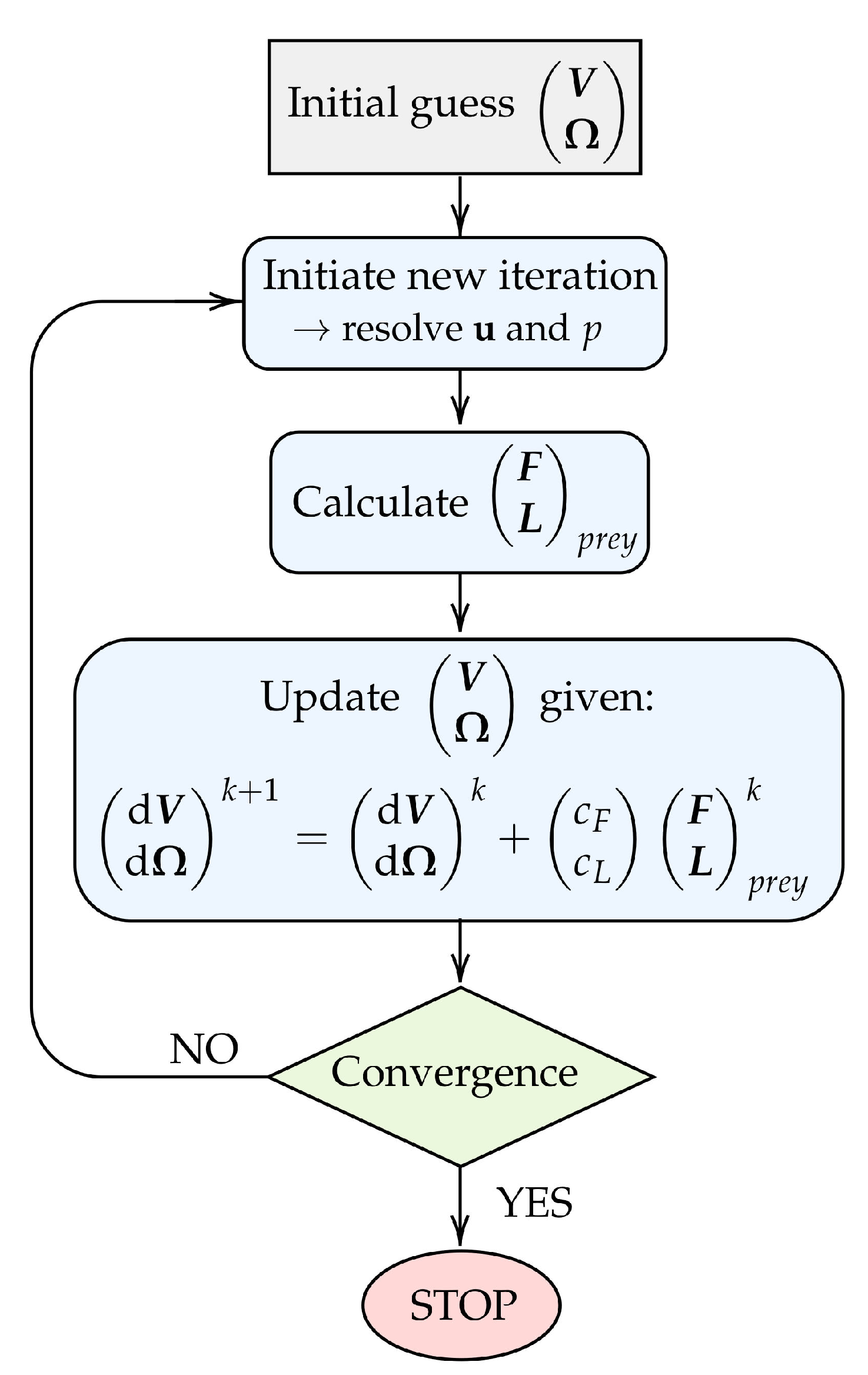
The procedure for obtaining the prey velocity and rotation rate in each discrete time step is illustrated in Figure 3. Firstly, an arbitrary initial guess is assigned to the unknown and . This allows for the flow velocity and pressure fields to be computed using the SIMPLE algorithm [20]. Subsequently, the forces and torques acting on the prey surface can be deduced. Given the prey forces and torques, we update the prey velocity and rotation rate using the relation:
where k denotes an iteration counter and and are relaxation constants for the translational velocity and the rotation rate, respectively. The constants are arbitrarily chosen such that and are much smaller than and , respectively. The magnitude of and is found only to influence the rate of convergence, and we use throughout.
The updated prey velocity and rotation rate serve as the input for a new iteration, in which the above procedure is repeated. The iteration process continues until the forces and torques on the prey are converged to a negligible level. At this point, the prey position is updated based on the converged prey velocity and rotation rate. The entire procedure is repeated for the subsequent time step.
3. Results and Discussion
3.1. Static Analysis
In this section, we only consider fixed prey. All simulations are carried out for all 12 positions on the collar, as described in Section 2.1.1, for both the loricate and non-loricate D. grandis. Firstly, the effect of placing a prey exactly behind a microvilli tentacle is compared to the effect of letting it rest in between two tentacles (not shown). We find a significant amplification of measured forces on the prey when placed directly in the flow between two tentacles. Assuming that the prey particles follow the streamlines of the flow [19], it seems reasonable to assume that the equilibrium position of a captured bacterial prey is between any neighboring pair of microvilli tentacles. Thus, all static analyses are simulated accordingly.
3.1.1. Prey Positions on the Collar Filter
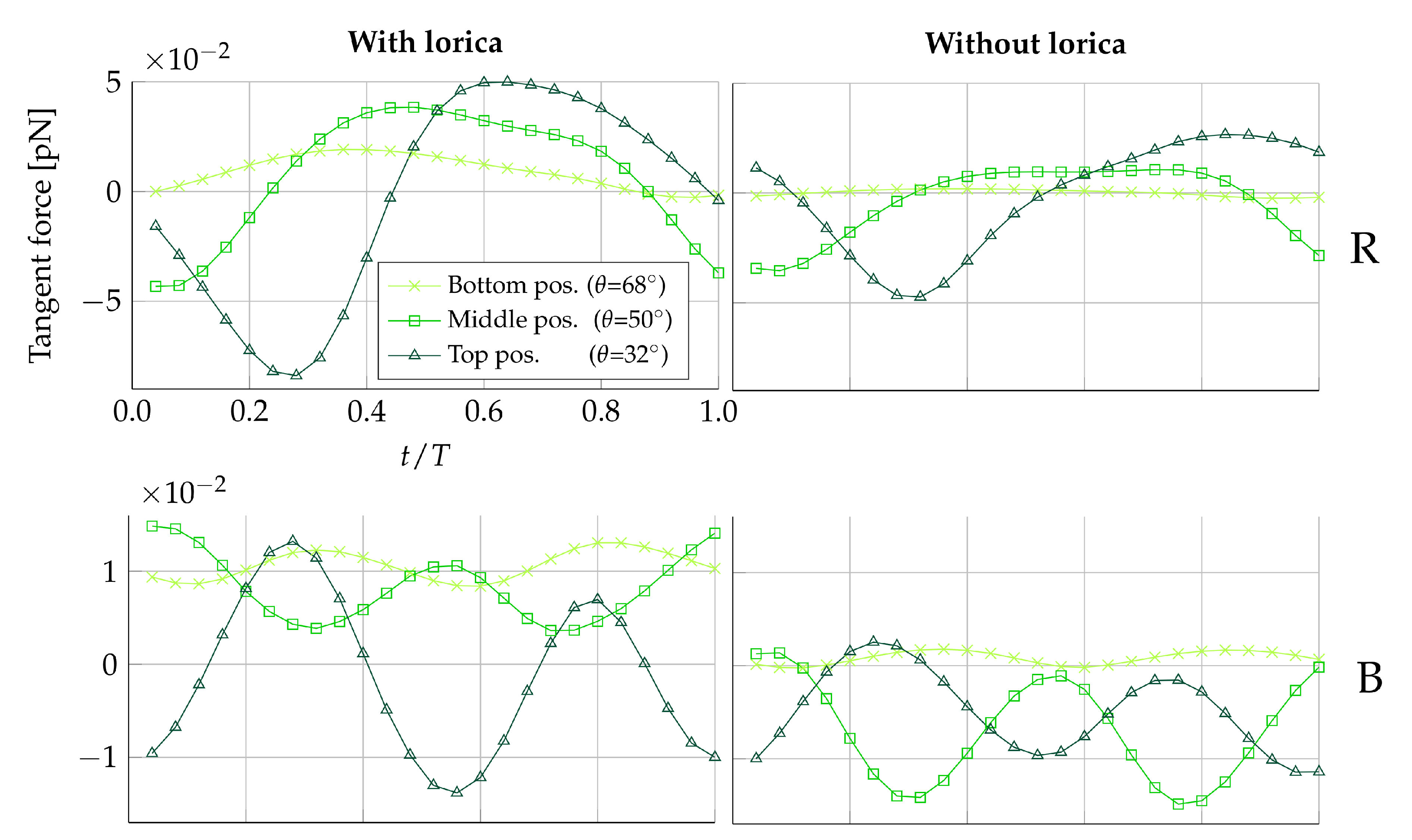
Figure 4 shows the tangent force on for the duration of one beat cycle. Due to the symmetry in the ambient flow between prey placed in the same plane but on opposite sides of the collar, only one prey from each of the beat and the vane planes is shown ( and ). Figure 4 suggests that the magnitude of the force exerted on the prey by the fluid is amplified when the prey is positioned on the upper half of the collar, as compared to the lower half. Furthermore, observing the scale of the forces in Figure 4, it can be seen the tangential forces exerted on the prey by the fluid are approximately five times larger in magnitude in the beat plane compared to the vane plane. The force time history in each plane also differs over the course of a full beat cycle; in the beat plane, the rate of change of the force generally switches sign twice, whereas in the vane plane, the rate of change switches sign four times.
To provide an understanding of this difference in forces between the beat and vane plane, the underlying velocity fields are illustrated in Figure 5. In the beat plane (Figure 5A,B), it is apparent that at the lateral peaks of the sinusoidal vane displacement, a vortex appears. The vortex appearing to the left of the cell rotates counter-clockwise, and the vortex appearing to the right of the cell rotates clockwise. Consequently, the near-collar flow in the beat plane is directed downwards, as a flagellum peak sweeps by. It is observed that a change in the sign of the tangent prey force coincides with a change in the vertical direction of the near-prey flow. The velocity magnitude induced by the vortex is highest close to its center, which is located at the flagellum displacement peak. The magnitude gradually decreases when radially moving further away from the vortex center. Since the flagellum beats closer to the filter in the upper part of the collar, we hypothesize that this explains why the magnitude of force directed towards the cell (negative tangent force) is increased the higher up along the collar the prey is positioned. Other choanoflagellate species, such as the Salpingoeca rosetta, construct a straight rather than a curved collar, and subsequently, the proximity to the flagellar vane is increased [21]. Such species therefore present an opportunity to explore this hypothesis further. In the vane plane (Figure 5C), we find that a vortex appears along the vane edges at the two points in which the flagellar vane intersects the vane plane. Thus, this explains why the rate of change of the tangent is found to change sign four times during one beat cycle.
From Table 3, we find that the average beat cycle tangential force is directed towards the cell for in the loricate D. grandis and for both and in the non-loricate D. grandis. This trend is apparent in both the beat plane () and in the vane plane (). Despite the same overall trend being apparent in both planes, the two planes still perform differently. In the loricate case, the average tangential force is lower in the beat plane than in the vane plane for all vertical filter positions. The opposite is observed in the non-loricate case, where we find the lowest tangential forces in the vane plane. Since hydrodynamic transportability effects seem to vary between the two planes, we speculate that this could be the reason why it has been observed that, on occasion, prey traverse multiple microvilli as they descends toward the cell [12]. However, it remains elusive which circumferential position on the filter is most favorable in terms of prey transportability.
Hydrodynamics are only found to be beneficial to the transportability of prey towards the cell in the upper half of the filter. No aiding effects were found at the lower part of the collar. This lack of hydrodynamic effects could explain the presence of the observed lamellipod-like “collar skirt” structure that surrounds the collar base in the choanoflagellate species S. rosetta [6,12]. The function of the skirt has thus far remained unknown; however, we speculate that because hydrodynamics cannot aid the transportation of prey in the lower part of the collar filter, the function the skirt is to bridge the prey-handling process to phagocytosis, hence completing the prey capture process. The time series of the process of prey capture and ingestion ([12] Figure 1 therein) show that after the prey travels down the collar, it remains at the lower part of the collar (where the skirt is located) for ∼2 min before eventually being phagocytosed.
3.1.2. Prey Retention
In the non-loricate choanoflagellate species S. rosetta, microscopic imaging has revealed that bacteria often make contact with the collar and remain there for a short while, until escaping captivity and subsequently drifting away [12]. We find that hydrodynamics could potentially explain these observations. From Figure 5D, which shows the velocity field in the horizontal -plane at the collar position , it is apparent that in the beat plane, the flow field is directed away from the collar at some instance during a beat cycle. Further investigation of this flow behavior subsequently suggests that the water is pushed away from the collar by the flagellum peak displacement point. Hence, the motion of the flagellum simultaneously directs the flow field both outwards and down towards the cell when the flagellum peak passes the filter.
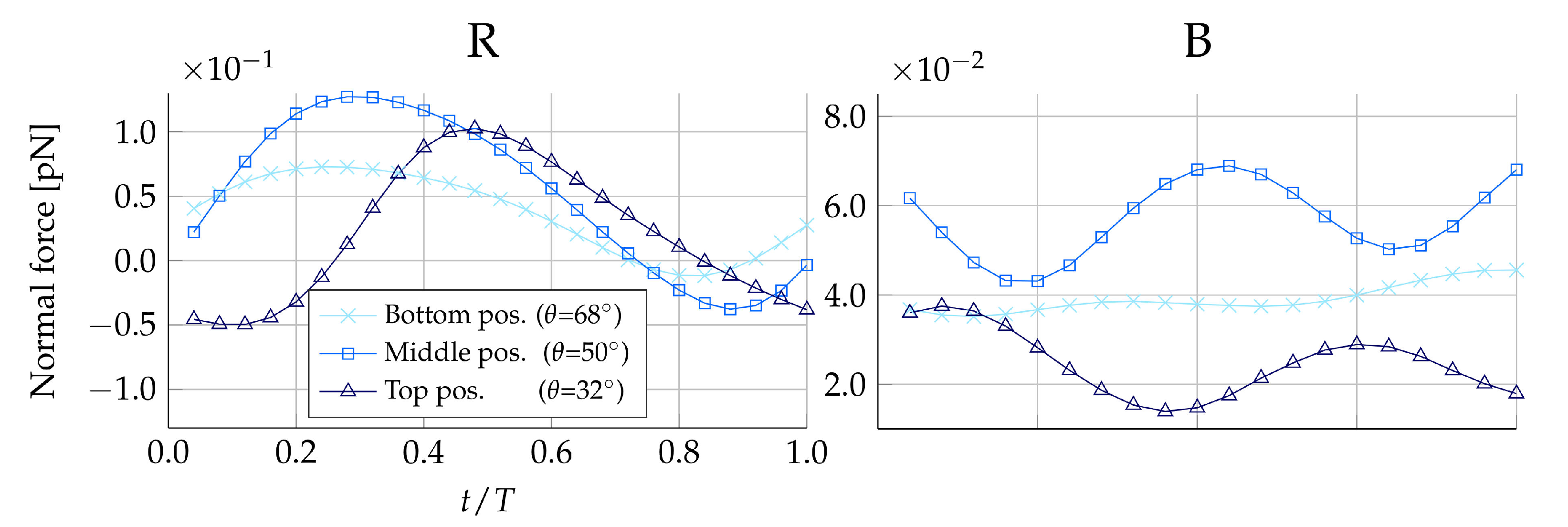
Figure 6 shows the variation in normal forces on during one flagellate beat cycle. For the non-loricate D. grandis, we find that the normal force in the beat plane changes direction twice in one cycle, and thus, as the flow field predicted, the prey experiences both forces that are directed towards and away from the collar within the duration of one beat cycle. Assuming hydrodynamics to be the main cause of prey loss, the normal forces give an indication of how strong the retention effect of the microvilli tentacle surface should be. We find that for , the contact forces between the prey and the microvilli should exceed to overcome the counteracting hydrodynamic forces. The equivalent minimum contact forces found for the other prey types are shown in Table 4.
In the vane plane, we find the normal forces to be orientated towards the collar at all times. However, we note that the vortex along the flagellar vane sheet edge constantly alters the direction of the nearby flow. Hence, the normal forces in the vane plane seem to be particularly dependent on the width of the flagellar vane sheet. Only a few choanoflagellate species have sporadically been pictured with a flagellar vane composed of a sheet-like structure due to the difficulty of capturing it with electron microscopy [5,22]. The exact shape of the sheet-like structure therefore remains elusive. Thus, due to the uncertainty in the shape and extent of the sheet-like structure, we cannot exclude the possibility that hydrodynamics could be counteracting the retention of prey in the vane plane as we find them to do in the beat plane.
3.1.3. Loricate Effect
The two columns in Figure 4 show the difference in tangential forces for a loricate and non-loricate D. grandis. Removing the lorica does not seem to have an effect on the overall trend of the force time history, though it does affect the magnitude of the simulated forces. In the vane plane (), it is especially noticeable that removing the lorica reduces the magnitude of the predicted forces. At some points in a beat cycle, the force reduction even leads to a change from a positive force to a negative force. Thus, this is an improvement in the degree of prey transportability. Observing Figure 5, it becomes apparent that the lorica directs the incoming flow field upwards, whereas in the non-lorica D. grandis, the flow reaches the collar at a more horizontal direction. Assuming equal flow magnitudes, it requires less force to direct a horizontally orientated flow downwards, as compared to directing an upwards-orientated flow downwards. Consequently, this explains why we see a reduction in the tangential forces for the non-loricate D. grandis in Figure 4. Furthermore, it is observed that the amplitude of the force magnitude is generally reduced in the non-loricate case as compared to the loricate case. We find no direct explanation for this. However, it seems probable that the cause could be related to either the orientation of the flow near the collar or a shielding effect from the presence of the lorica.
In the loricate D. grandis, we find from Table 3 that the most favorable position, in terms of the strongest degree of prey transportability in the direction of the cell, is at the top of the collar. When removing the lorica, we still see a transportation effect directed towards the cell at the top of the collar, but the position in which the effect is highest is now at the middle of the collar. This observation contradicts our previous hypothesis, which suggested that the proximity to the flagellum is positively correlated to the subsequent degree of prey transportability. We find no apparent trend that explains why the middle position on the collar is the most favorable position in terms of prey transportability in the non-loricate case. However, we speculate that it could be related to the position of the induced vortex relative to the filter, as the vortex is influenced by the presence of the lorica.
Given that D. grandis is a loricate choanoflagellate, we subsequently conclude that the adaptive value of the lorica does not seem to be an improvement in the hydrodynamic transportability of prey. It rather seems that the adaption of the lorica results in a deterioration of such effects. However, hydrodynamics could still act as an aiding factor for the unknown means of prey transportation.
3.1.4. Prey Size and Shape
When varying the size of the prey, one would also expect to see a change in forces from the flow on the prey. An increased force in the direction towards the cell is not necessarily advantageous for the transportability of prey. Likewise, a reduced force does not have to be disadvantageous. The prey velocity also depends on the shape and size of the prey, which could negate or weaken effects of increased or reduced forces on the prey. We use the Stokes law in Equations (10) and (11) to transform the simulated tangent forces on the four different prey types (Table 2) into their respective tangent velocities. We note that the force contributions from pressure and viscous forces are approximately 1:1 for all prey types during one beat cycle. This suggests that we do not have a perfectly symmetric flow around the prey [15], which stems from disturbances induced by the proximity of the collar. Hence, the Stokes law cannot act as an accurate approximation of the velocity magnitude, but may still suffice as an approximation of the order of magnitude.
The time-averaged tangent force for one beat cycle is listed in Table 3 for each prey type in the beat plane () and in the vane plane (). The resultant tangent velocities can be seen in Figure 7. The tangent velocities that are directed towards the cell (negative velocities) are observed to be in the approximate range of –. Given that the length of one microvilli is ∼9, the time it would take to move a prey from the very top of the collar to the cell, assuming constant velocities within this velocity range, is 7–. For the non-loricate choanoflagellate S. rosetta, with an approximate collar height of [21], the movement of bacterial prey down along the collar has been observed to take , on average, after the first point of contact between the prey and the collar [12]. Given that the first point of contact with the collar is at an arbitrary position, these physical observations seem to be in good agreement with the order of the resultant tangent prey velocities found in this static part of the study (Figure 7).
When comparing the effects of varying the prey size and shape, we find that elongating a prey in the direction parallel to the tangent of the collar surface () seems to have an insignificant effect on its resulting velocity, as compared to its original spherical shape (). Similarly, decreasing the size of the prey () is found to result in a slight decrease in velocity magnitude. Enlarging the prey () is, on the other hand, found to have a significant effect on the transportability of prey. In the loricate D. grandis, the results indicate that there is no apparent place on the collar in which is moved in the direction of the cell when considering its average velocity in one beat cycle. Similarly, the transportability of prey in the non-loricate D. grandis is significantly decreased for when compared to the other prey types investigated. The larger the size of the fixed prey particle, the more it is going to alter the local flow field as compared to when it is free to drift. Hence, for , we conclude that hydrodynamics can have a positive effect on the transportability of prey, even though such an effect is not apparent in this static analysis.
3.2. Dynamic Analysis
In this section, which covers the dynamic approach, prey will be allowed to move freely within the flow. We will consider the prey velocity components at some of the same positions on the collar that were considered in the static study. From these positions, we take one time step of a negligible size () such that the velocity components are essentially evaluated in their initial position. The flagellum positions at the instant in time at which we evaluate the velocities are pictured in Figure 1. We iterate through the solution procedure given in Figure 3 until all forces and torques on the prey have converged to a level of, at most, 0.1% of the resultant translational and rotational prey velocities (Supplementary Information S8.4). Here, the comparison is made possible using the Stokes law. We only consider and in the setting of the loricate D. grandis.
Freely Drifting Prey
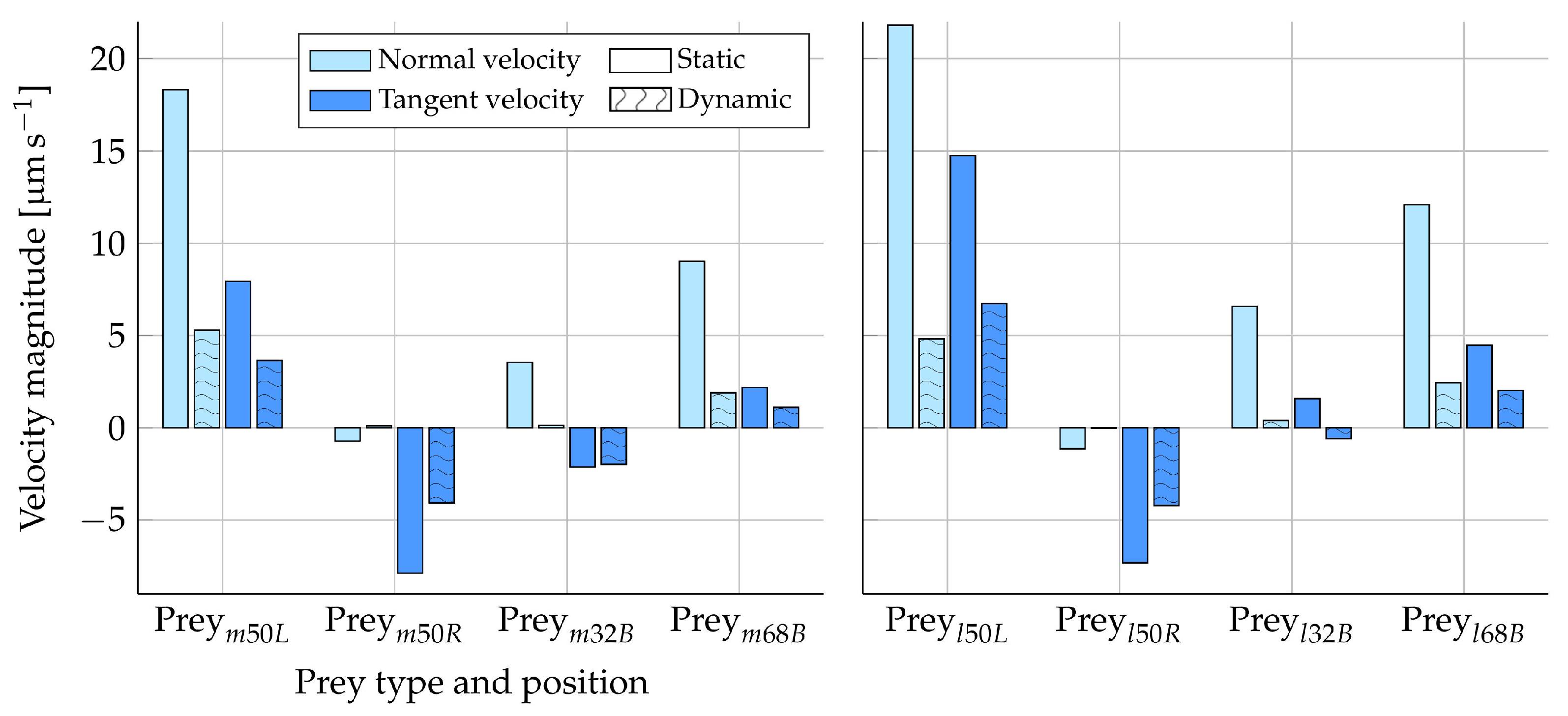
Figure 8 shows the difference in the tangent and normal prey velocity between the static and dynamic analysis. The Stokes law (Equation (10)) is expected to give an overestimation of the prey velocities calculated from prey forces due to the boundary effects of the nearby microvilli (Section 2.1.2). In Figure 8, it can be observed that the velocities are generally evaluated to a higher value in the static simulations as compared to the dynamic simulations. This trend is therefore consistent with our prior expectations. The directions of the velocity components are also found to be the same in both the static and dynamic analysis, with the exception of some near-zero velocities. Considering only the tangent velocities for , the static simulations overestimate the prey velocity magnitude by, at most, approximately two times as compared to the dynamic results.
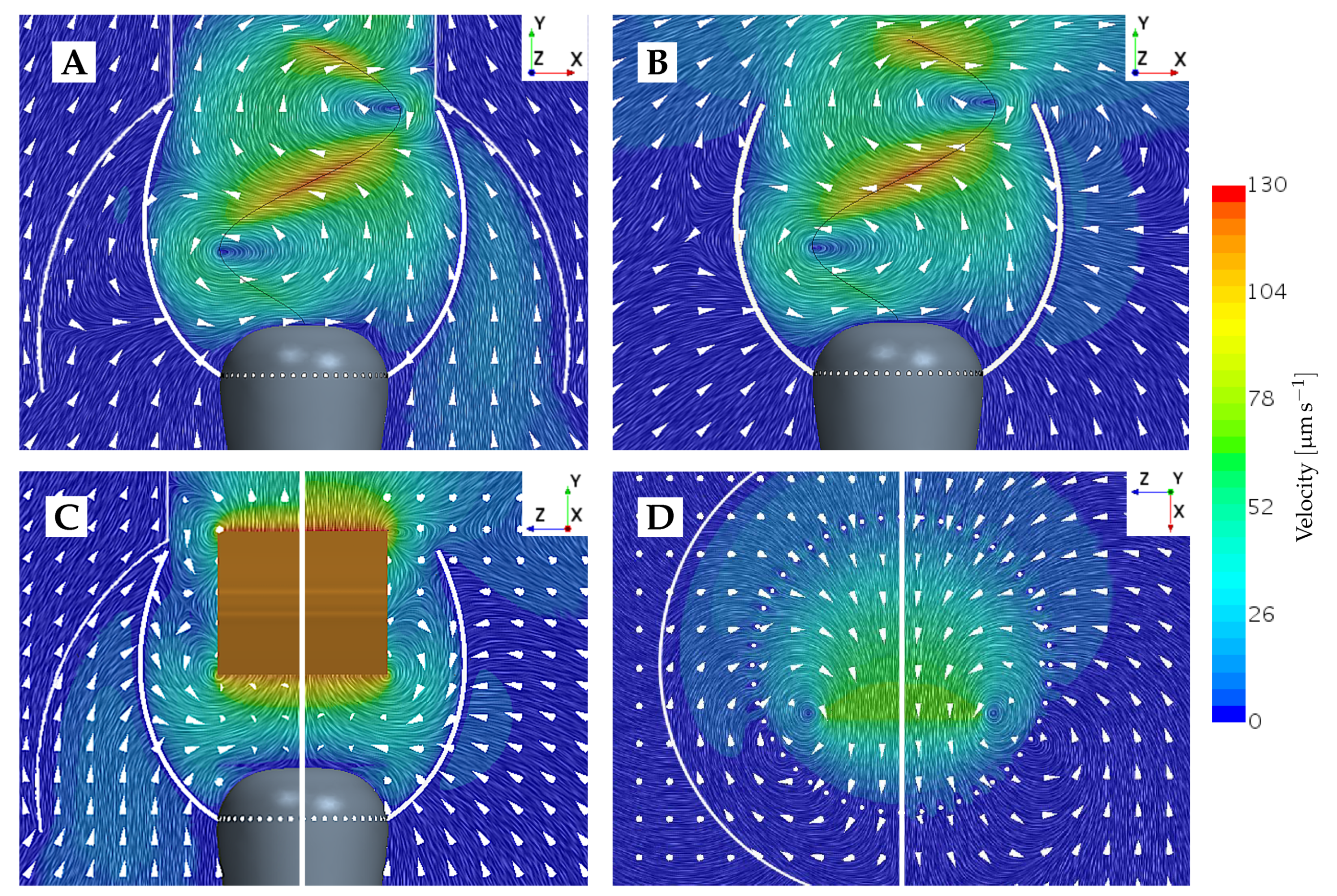
The normal velocity component obtained for from the static and dynamic approaches seems less comparable than the tangent velocity results, judging by Figure 8. However, both approaches still evaluate the magnitude of the normal velocities to be within the same order. Considering , the static and dynamic results vary more compared to , which is expected due to the bigger impact that a larger particle has on the local flow field. Hence, we expect the static and dynamic results to vary more when increasing the prey size, which is the trend that is observed. The resultant local flow fields when fixing , as compared to letting it freely drift, are shown in Figure 9. Considering Figure 9A,B, we observe that the fixation of the prey gives rise to a change in the flow direction from upstream to downstream around the prey. This non-trivial change in the velocity field may cause a change in the resultant force on the prey. Hence, the artificial motion of the fixed prey (as predicted by the Stokes law) will be different from that of the freely drifting prey. In Figure 9C,D, the flow field direction around the fixed prey is not changed as drastically, as seen in Figure 9A,B. However, Figure 9 only considers a discrete instance in time at a certain collar position. Therefore, the figure only confirms and visualizes that the fixation of prey does, in fact, alter the local flow field to an extent that seems significant to the prey motion.
The variation found between the static and dynamic results could be a result of the coupling between the prey rotation and translation. Due to the proximity of the microvilli, the symmetry in the flow around the spherical prey is disturbed [23]. This disturbance is accounted for in the dynamic analysis, where the torque on the prey surface is considered in addition to the forces. However, the static analysis only considers prey surface forces. From the dynamic analysis, we find that prey generally rotate around their local z-axis at the positions on the collar considered in Figure 8. This suggests that the tangential translation of the prey relative to the collar surface would be most impacted by the prey rotation. In order to evaluate the degree of the impact on the prey’s translation caused by its own rotation, we also simulate the motion of a constrained prey that is allowed to have only translational velocity. Each resultant velocity component is found to vary up to 6% compared to those of a freely drifting prey (Figure 8). We find the biggest variations in the tangent velocity components, as we expected, from the axis about which the prey generally rotate. The small variation in results suggests that the prey rotation and translation can be considered to be decoupled, and subsequently, the variation in the static and dynamic results cannot be due to neglecting the rotation in the static approach.
Based on the results from the dynamic study, we remain confident that there exists a hydrodynamic effect that could be an aiding factor in the process of transporting prey to the cell. Furthermore, we trust the order of magnitude of the results obtained through the static study, but acknowledge that the static results seem to be overestimations when compared to the dynamic results. Since only spherical prey were considered in the dynamic approach, we cannot validate the static results for . Here, due to the asymmetrical shape of the prey, rotation might have a bigger impact than what was found for spherical prey. The rotation of will also depend on its orientation on the collar. In the static analysis, we assumed the major axis of to be parallel with the downwards-orientated tangent vector on the collar surface. Given that the prey rotates, it is likely to see the orientation changes over the course of a beat cycle. Hence, a complete analysis of the motion of elongated prey is rather complex and is beyond the scope of the present study.
4. Conclusions
In this study, which considered finite-sized prey, our results suggest that, at some positions on the feeding collar, hydrodynamics do contribute to the transportability of prey in the direction towards the cell. The results do not indicate that hydrodynamics account for the majority of the transportability of prey; they rather suggest that hydrodynamics could be an aiding factor in the main means of prey transportation, the nature of which remains unknown. Removing the lorica was found to increase the extent of the region on the collar surface at which hydrodynamics positively impact the prey transportability. Thus, the adaptive value of the lorica does not seem to be linked to the transportability of prey.
Supplementary Materials
The following are available online at https://0-www-mdpi-com.brum.beds.ac.uk/2311-5521/6/3/94/s1, Figure S1: Model residuals, Figure S2: Convergence of mesh size, Figure S3: Mesh illustrations, Table S1: Morphology parameters.
Author Contributions
Conceptualization S.S.A. and J.H.W.; methodology S.S., S.S.A. and J.H.W.; software S.S., S.S.A. and J.H.W.; validation S.S. and S.S.A.; writing S.S. and S.S.A.; review and editing S.S., S.S.A. and J.H.W.; supervision S.S.A. and J.H.W.; funding acquisition J.H.W. All authors have read and agreed to the published version of the manuscript.
Funding
We gratefully acknowledge funding from the Villum Foundation for S.S.A. and J.H.W. through a research grant (9278).
Acknowledgments
We thank Anders Andersen, Thomas Kiørboe, Bo Gervang, and Poul Scheel Larsen for the fruitful discussions on prey capture at low Reynolds numbers and Lasse Tor Nielsen for providing images of D. grandis.
Conflicts of Interest
The authors declare no conflict of interest.
References
- Sherr, E.B.; Sherr, B.F. Significance of predation by protists in aquatic microbial food webs. Antonie Van Leeuwenhoek 2002, 81, 293–308. [Google Scholar] [CrossRef] [PubMed]
- Leadbeater, B.S.C. The Choanoflagellates: Evolution, Biology and Ecology, 1st ed.; Cambridge University Press: Cambridge, UK, 2015. [Google Scholar]
- Lang, B.F.; O’Kelly, C.; Nerad, T.; Gray, M.W.; Burger, G. The closest unicellular relatives of Animals. Curr. Biol. 2002, 12, 1773–1778. [Google Scholar] [CrossRef] [Green Version]
- Kiørboe, T. How zooplankton feed: Mechanisms, traits and trade-offs. Biol. Rev. 2011, 86, 311–339. [Google Scholar] [CrossRef] [PubMed]
- Nielsen, L.T.; Asadzadeh, S.S.; Dölger, J.; Walther, J.H.; Kiørboe, T.; Andersen, A. Hydrodynamics of microbial filter feeding. Proc. Natl. Acad. Sci. USA 2017, 114, 9373–9378. [Google Scholar] [CrossRef] [PubMed] [Green Version]
- Mah, J.L.; Christensen-Dalsgaard, K.K.; Leys, S.P. Choanoflagellate and choanocyte collar-flagellar systems and the assumption of homology. Evol. Dev. 2014, 16, 25–37. [Google Scholar] [CrossRef] [PubMed]
- Asadzadeh, S.S.; Larsen, P.S.; Riisgård, H.U.; Walther, J.H. Hydrodynamics of the leucon sponge pump. J. Roy. Soc. Inter 2019, 16, 20180630. [Google Scholar] [CrossRef] [PubMed] [Green Version]
- Pettitt, M.E.; Orme, B.A.A.; Blake, J.R.; Leadbeater, B.S.C. The hydrodynamics of filter feeding in choanoflagellates. Eur. J. Protist. 2002, 38, 313–332. [Google Scholar] [CrossRef] [Green Version]
- Asadzadeh, S.S.; Nielsen, L.T.; Dölger, J.; Andersen, A.; Kiørboe, T.; Larsen, P.S.; Walther, J.H. Hydrodynamic functionality of the lorica in choanoflagellates. J. Roy. Soc. Inter 2019, 16, 20180478. [Google Scholar] [CrossRef] [PubMed] [Green Version]
- Strathmann, R.R. Larval feeding in echinoderms. Am. Zool. 1975, 15, 717–730. [Google Scholar] [CrossRef]
- Bloodgood, R.A. Prey capture in protists utilizing microtubule filled processes and surface motility. Cytoskeleton 2020, 77, 500–514. [Google Scholar] [CrossRef] [PubMed]
- Dayel, M.; King, N. Prey Capture and Phagocytosis in the Choanoflagellate Salpingoeca rosetta. PLoS ONE 2014, 9, e95577. [Google Scholar] [CrossRef] [PubMed] [Green Version]
- Lauga, E.; Powers, T.R. The hydrodynamics of swimming microorganisms. Rep. Prog. Phys. 2009, 72, 096601. [Google Scholar] [CrossRef]
- Guazzelli, E.; Morris, J.F. A Physical Introduction to Suspension Dynamics; Cambridge University Press: Cambridge, UK, 2012. [Google Scholar]
- White, F.M. Viscous Fluid Flow, 3rd ed.; McGraw Hill, Inc.: New York, NY, USA, 2006. [Google Scholar]
- Oberbeck, A. Ueber stationäre Flussigkeitsbewegungen mit Berucksichtigung der inneren Reibung. Crelles J. 1878, 81, 62–80. [Google Scholar]
- Clift, R.; Grace, J.; Weber, M.E. Bubbles, Dropls, and Particles; Dover Publication Inc.: Miniola, NY, USA, 1978. [Google Scholar]
- Panton, R.L. Incompressible Flow, 4th ed.; John Wiley & Sons: Hoboken, NJ, USA, 2013. [Google Scholar]
- Homann, H.; Guillot, T.; Bec, J.; Ormel, C.W.; Ida, S.; Tanga, P. Effect of turbulence on collisions of dust particles with planetesimals in protoplanetary disks. Astron. Astrophys. 2016, 589, A129. [Google Scholar] [CrossRef] [Green Version]
- Patankar, S.V. Numerical Heat Transfer and Fluid Flow; Hemisphere: Dublin, OH, USA, 1980. [Google Scholar]
- Dayel, M.; Alegado, R.; Fairclough, S.; Levin, T.; Nichols, S.; McDonald, K.; King, N. Cell differentiation and morphogenesis in the colony-forming choanoflagellate Salpingoeca Rosetta. Dev. Biol. 2011, 357, 73–82. [Google Scholar] [CrossRef] [PubMed] [Green Version]
- Leadbeater, B.S.C. The mystery of the flagellar vane in choanoflagellates. Nova Hedwig. Beih. 2006, 130, 213. [Google Scholar]
- Batchelor, G.K.; Green, J.T. The hydrodynamic interaction of two small freely-moving spheres in a linear flow field. J. Fluid Mech. 1972, 56, 375–400. [Google Scholar] [CrossRef]
Figure 1.
Morphology of Diaphanoeca grandis. (A) Microscopic image of the choanoflagellate. Scale bar: . (B) Model morphology picturing the cell (green), collar filter (red), flagellum (yellow), and lorica dome and chimney (blue) with ribs (gray) in the lower part of the lorica. The direction of the flow is indicated with the dashed arrows.

Figure 2.
(A) The 3D computational fluid dynamics (CFD) model morphology, shown with a wide flagellar vane (yellow) and a medium-sized prey (gray). (B) A 2D schematic of the CFD model. The bold curves, which correspond to Equations (2) and (3), are revolved around the longitudinal center axis to create the model surfaces (pictured as opaque). The polar coordinate system, which is shown in degrees, serves as the reference frame for the prey’s placement along the filter collar. (C) The three vertical prey positions on the collar. Each prey (gray) is equipped with a local coordinate system: normal (x) and tangent (y) to the collar surface. Pictured is a medium-sized prey (gray) in true relative scale.

Figure 3.
Flowchart illustrating the iterative procedure used to model drifting prey. The chart covers the process for one arbitrary discrete time step. Here, k denotes an iteration counter.
Figure 3.
Flowchart illustrating the iterative procedure used to model drifting prey. The chart covers the process for one arbitrary discrete time step. Here, k denotes an iteration counter.

Figure 4.
Tangent force distribution on medium-sized prey during one beat cycle with period T. Here, negative forces are in the direction of the cell. The left-hand column of plots is simulated with the presence of the lorica, and the right-hand column of plots is simulated without. The first row of plots displays forces on the right (R) side of the the collar, and the second row displays forces on the back (B) of the collar.

Figure 5.
Planar views of an instantaneous flow field velocity simulated without the presence of prey. (A) Beat plane view with the lorica. (B) Beat plane view without the lorica. (C) Vane plane view with and without the lorica, respectively. (D) Horizontal view through the collar at position , pictured with and without the lorica, respectively.

Figure 6.
Normal force distribution on medium-sized prey during one beat cycle with period T. Here, negative forces are orientated in the direction away from the collar. Both plots are simulated without the presence of the lorica. The left-hand plot shows the forces on prey placed on the right (R) side of the collar, and the right-hand plot shows forces on prey placed at the back (B) of the collar.

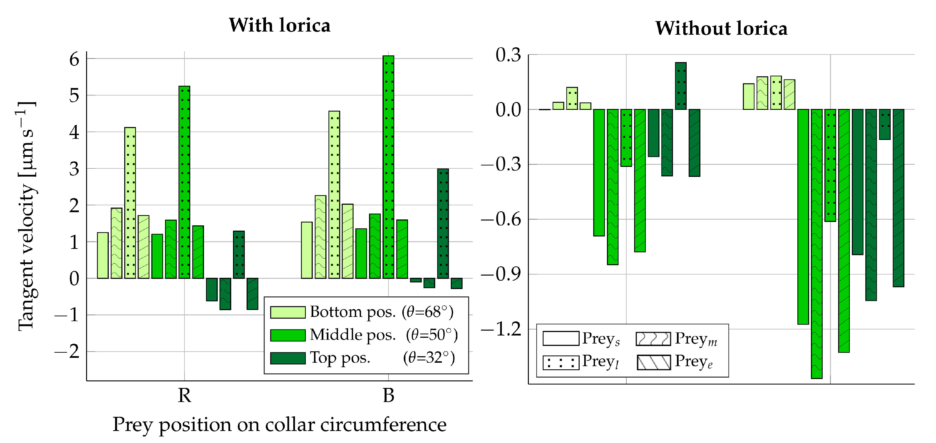
Figure 7.
Resultant tangent velocity of fixed prey when using Equations (10) and (11) to convert simulated forces (Table 3) into velocities. Here, a negative velocity is directed towards the cell. The left plot is simulated with the lorica and the right plot without. Velocities are shown for prey placed in the beat plane on the right (R) side of the collar and in the vane plane on the back (B) side of the collar. For each vertical position on the collar (), the velocity is shown for each type of prey considered: small (s), medium (m), large (l), and elongated (e). The two legends apply to both plots.

Figure 8.
Prey velocity components in the normal and tangent directions to the collar from both the static and dynamic analyses. A prey was placed on the middle and left-hand side of the collar (), the middle and right-hand side (), the top and back side (), and the bottom and back side (). The left plot shows the results for a medium-sized prey, and the right plot shows the results for a large-sized prey. All results were simulated with the presence of the lorica and at the flagellum position pictured in Figure 1.

Figure 9.
Planar views of the flow field velocity near a prey, showing the differences between the static and dynamic simulation approaches. Pictured is the large prey positioned on the left side of the filter around the middle () using the local prey coordinate system. All figures show the instantaneous flow field corresponding to the flagellum position pictured in Figure 1. (A) The local flow field seen from a frontal perspective when the prey is fixed. (B) The local flow field seen from a frontal perspective when the prey freely drifts. (C) The local flow field seen from a top perspective when the prey is fixed. (D) The local flow field seen from a top perspective when the prey freely drifts.


Table 1.
Characteristic flagellum parameters specific to D. grandis. A is the wave amplitude, L is the projected length of the flagellum onto the center axis y, f is the wave frequency, is the wavelength, and W is the width of the flagellar vane.
Table 1.
Characteristic flagellum parameters specific to D. grandis. A is the wave amplitude, L is the projected length of the flagellum onto the center axis y, f is the wave frequency, is the wavelength, and W is the width of the flagellar vane.
| 2.8 | 8.3 | 7.3 | 8.6 | 5.0 |
Table 2.
Characteristic parameters of the four different prey types considered: small, medium, large, and elongated, denoted by s, m, l, and e, respectively. Dimensions are given in μm. Only is smaller than the filter openings.
Table 2.
Characteristic parameters of the four different prey types considered: small, medium, large, and elongated, denoted by s, m, l, and e, respectively. Dimensions are given in μm. Only is smaller than the filter openings.
| Major radius | 0.18 | 0.25 | 0.50 | 0.50 |
| Minor radius | - | - | - | 0.25 |
Table 3.
Time-averaged tangent forces on prey during one flagellum beat cycle for both the loricate and the non-loricate choanoflagellate. One position in the beat plane (R) and one position in the vane plane (B) are shown. Column-wise, the table depicts the effects of prey size and shape variations. Row-wise, the effects of the longitudinal position on the collar () can be seen.
| Average Tangent Force per Beat Cycle | ||||||
|---|---|---|---|---|---|---|
| Case | ||||||
| Beat plane (R) | with lorica | 68 | 4.2 | 9.0 | 38.8 | 11.3 |
| 50 | 4.1 | 7.5 | 49.4 | 9.4 | ||
| 32 | −2.1 | −4.0 | 12.1 | −5.6 | ||
| without lorica | 68 | 0 | 0.2 | 1.1 | 0.2 | |
| 50 | −2.3 | −4.0 | −2.9 | −5.1 | ||
| 32 | −0.9 | −1.7 | 2.4 | −2.4 | ||
| Vane plane (B) | with lorica | 68 | 5.2 | 10.7 | 43.0 | 13.3 |
| 50 | 4.6 | 8.3 | 57.2 | 10.5 | ||
| 32 | −0.3 | −1.2 | 28.2 | −1.8 | ||
| without lorica | 68 | 0.5 | 0.8 | 1.7 | 1.1 | |
| 50 | −4.0 | −6.9 | −5.8 | −8.8 | ||
| 32 | −2.7 | −4.9 | −1.6 | −6.4 | ||
Table 4.
Minimum contact force between microvilli tentacles and prey required to counteract the simulated hydrodynamic normal forces in the non-loricate D. grandis.
Table 4.
Minimum contact force between microvilli tentacles and prey required to counteract the simulated hydrodynamic normal forces in the non-loricate D. grandis.
| Min. contact force [pN] | 0.03 | 0.05 | 0.10 | 0.08 |
Publisher’s Note: MDPI stays neutral with regard to jurisdictional claims in published maps and institutional affiliations. |
© 2021 by the authors. Licensee MDPI, Basel, Switzerland. This article is an open access article distributed under the terms and conditions of the Creative Commons Attribution (CC BY) license (http://creativecommons.org/licenses/by/4.0/).
Share and Cite
MDPI and ACS Style
Sørensen, S.; Asadzadeh, S.S.; Walther, J.H. Hydrodynamics of Prey Capture and Transportation in Choanoflagellates. Fluids 2021, 6, 94. https://0-doi-org.brum.beds.ac.uk/10.3390/fluids6030094
AMA Style
Sørensen S, Asadzadeh SS, Walther JH. Hydrodynamics of Prey Capture and Transportation in Choanoflagellates. Fluids. 2021; 6(3):94. https://0-doi-org.brum.beds.ac.uk/10.3390/fluids6030094
Chicago/Turabian StyleSørensen, Siv, Seyed Saeed Asadzadeh, and Jens Honoré Walther. 2021. "Hydrodynamics of Prey Capture and Transportation in Choanoflagellates" Fluids 6, no. 3: 94. https://0-doi-org.brum.beds.ac.uk/10.3390/fluids6030094