
Cross Diffusion Effect on Linear and Nonlinear Double Diffusive Convection in a Viscoelastic Fluid Saturated Porous Layer with Internal Heat Source

Department of Basic Sciences and Mathematics, Faculty of Science, Philadelphia University, Amman 19392, Jordan
Fluids 2021, 6(5), 182; https://0-doi-org.brum.beds.ac.uk/10.3390/fluids6050182
Submission received: 16 March 2021
/
Revised: 2 May 2021
/
Accepted: 6 May 2021
/
Published: 12 May 2021
(This article belongs to the Special Issue Convection in Fluid and Porous Media)
Abstract
:Double diffusive convection in a binary viscoelastic fluid saturated porous layer in the presence of a cross diffusion effect and an internal heat source is studied analytically using linear and nonlinear stability analysis. The linear stability theory is based on the normal mode technique, while the nonlinear theory is based on a minimal representation of truncated double Fourier series. The modified Darcy law for the viscoelastic fluid of the Oldroyd type is considered to model the momentum equation. The onset criterion for stationary and oscillatory convection and steady heat and mass transfer have been obtained analytically using linear and nonlinear theory, respectively. The combined effect of an internal heat source and cross diffusion is investigated. The effects of Dufour, Soret, internal heat, relaxation and retardation time, Lewis number and concentration Rayleigh number on stationary, oscillatory, and heat and mass transport are depicted graphically. Heat and mass transfer are presented graphically in terms of Nusselt and Sherwood numbers, respectively. It is reported that the stationary and oscillatory convection are significantly influenced with variation of Soret and Defour parameters. An increment of the internal heat parameter has a destabilizing effect as well as enhancing the heat transfer process. On the other hand, an increment of internal heat parameter has a variable effect on mass transfer. It is found that there is a critical value for the thermal Rayleigh number, below which increasing internal heat decreases the Sherwood number, while above it increasing the internal heat increases the Sherwood number.
1. Introduction
Mathematical modeling of double-diffusive free convection in a fluid-drenched porous module has increased in popularity over the last few decades due to its numerous applications in diverse contexts, including nuclear waste repository, impurities within water resources, atmospheric effluents, material processing, oil reservoir modeling, geothermal fields, and biochemical processes. The thermal instability of a Newtonian fluid-drenched porous module was initially investigated by [1] and by Lapwood [2] using linear stability analysis. Their results were further authenticated experimentally by Elder [3] and Katto [4]. On the other hand, Ingham and Pop [5], Vafai [6] and Nield and Bejan [7] conducted comprehensive reviews of pertinent literature and the fundamental applications of thermal performance in a porous medium. External regulation of convection streams is important for enhancing or diminishing the flow performance in physical systems. At present, several techniques are used for controlling the convective instability of such systems, including those based on gravity, rotation, thermal modulation and imposed magnetic field. In their studies, Gershuni et al. [8] and Gresho and Sani [9] investigated the effect of gravity modulation in a differentially heated fluid module. Their findings indicate that the undesirable buoyancy-driven flows in a differentially heated fluid layer can be effectively stabilized by appropriate vertical vibrations. Similarly, Malashetty and Padmavathi [10] investigated the stability solution of a fluid-drenched porous module depending on the amplitude of vertical vibrations. These authors found that low-frequency vertical vibrations significantly affected the system stability limits. The magnetic field effect on double-diffusive convection in a micropolar nanofluid was established by Abidi et al. [11], who found that the heat and mass transfer are influenced by the increasing Hartman number. More recently, Kumar et al. [12] examined a weak nonlinear heat transfer in a viscoelastic fluid-saturated porous medium under the effect of rotational modulation and found that a modified Prandtl number suspends the heat transfer process. Flow and heat transfer in non-Newtonian nanofluids over porous surfaces was studied by Maleki et al. [13], who found these nanofluids to be superior to their Newtonian counterparts for injection and impermeable plates. The authors also noted that, in injection, the heat transfer can be decreased by utilizing non-Newtonian nanofluids. In an earlier study, Govender [14] discussed the effect of g-jitter on convection in a differentially heated homogeneous porous module and predicted the exact changeover point from the synchronous to the subharmonic solution by plotting Mathieu’s stability charts. These results were subsequently confirmed by Saravanan and Purusothaman [15], who also studied the effects of anisotropy parameters of a porous module subjected to vertical vibrations using the Brinkman model. Thermal convection instability in a mushy layer subject to vertical vibration has been examined by Srivastava and Bhadauria [16] using linear stability analysis. These authors discussed the influence of pertinent parameters on mushy layer stability. A large number of fundamental studies on the stability of a rotating fluid-saturated porous module has also been conducted due to its diverse industrial requirements and applications. Govender [17] and Malashetty and Swamy [18] provided a detailed overview of rotating fluid-saturated porous module characteristics and applications. On the other hand, Maleki et al. [19] focused on the influences of radiation and slip boundary conditions on heat transfer over a porous plate. They also examined the effect of nanoparticles on nanofluid flow and heat transfer and noted significant changes in heat generation, viscous dissipation and radiation, which led to a decrease in heat transfer.
Some fluids found in foodstuffs, medicines, polymers and paints are of intricate rheological nature, and can thus be considered viscoelastic fluids for the purpose of modeling, in which case a viscoelastic model rather than the Newtonian model should be adopted. Thermal instability in a viscoelastic fluid was initially considered by Herbert [20] and Green [21]. Several studies in this domain focused on buoyancy-driven thermal instability in a viscoelastic fluid-drenched porous module, including those published by Kim et al. [22], Malashetty et al. [23], Naryana et al. [24], Bhadauria and Kiran [25], and Altawallbeh et al. [26]. The stability of double-diffusive convection of a Maxwell fluid in a porous module has also been widely investigated over the last few decades. For instance, Awad et al. [27], Wang and Tan [28], and Zhao et al. [29] found that the Maxwell fluid properties exert a significant influence on system stability. There are numerous practical situations in which the convective stability of the porous module can be compromised when subjected to an internal heat source, as is the case of electrometallurgical development for treating spent nuclear fuel, radioactive decay of unstable isotopes and exothermic reaction in porous materials. The onset of convection in a porous module with an interior heat source was examined by Parthiban and Parthiban [30], Bhadauria [31], Altawallbeh et al. [32], and Badruddin [33], among other authors. Recently, Altawallbeh et al. [34] examined the influence of a magnetic field on the instability of a fluid layer saturated with a viscoelastic fluid with an internal heat source. These authors found that the magnetic field has a stabilizing effect in such cases. Similarly, Rana and Khurana [35] studied the thermoconvective instability of a water-based nanofluid layer in the presence of a magnetic field when the fluid and nanoparticles are in a local thermal non-equilibrium. They found that the isotherms for both fluid and particle phases are flattened near the wall, suggesting an increase in the convection within the nanofluid layer. The effects of internal heat on the instability of an inclined anisotropic porous layer were investigated by Storesletten and Rees [36]. They found that the onset criteria in the porous layer were influenced by both the anisotropy parameter and the inclination angle. Maleki et al. [37] studied the influence of heat generation and viscous dissipation on heat transfer and the fluid flow of pseudo-plastic nanofluid over a moving permeable plate. These authors observed that, for both Newtonian and non-Newtonian nanofluids, the local Nusselt number decreased as the injection parameter, heat generation or volume fraction of nanoparticles increased.
The concurrent process of heat and mass transfer in a fluid can be studied by applying the theory of temperature gradient, concentration gradient and material composition, which causes density variances and thus implicitly induces the fluid to the flow. Heat flux generated due to the variance in concentration is denoted as thermal diffusion or the Soret effect, and mass flux resulting from the variance in temperature is referred to as the Dufour effect, both of which are highly relevant to chemical engineering, petrology, hydrology, disposal of nuclear waste, geosciences, and so on. The cross-diffusion effects in a porous module have been extensively studied. For example, Taslim and Narusawa [38] established a connection between the cross-diffusion problem and double-diffusion problem in a porous module. On the other hand, Rudaraiah and Siddheshwar [39] evaluated nonlinear double-diffusive convection in a porous module subject to Soret and Dufour effects. Many researchers have also investigated the effect of cross-diffusion coefficients on the double-diffusion convection in a porous module. Specifically, Gaikwad et al. [40] focused on the influence of cross-diffusion on linear and nonlinear double-diffusive convection in a fluid-saturated anisotropic porous layer. The Soret effect on double-diffusive convection in a couple-stress fluid-saturated porous medium was reported by Malashetty et al. [41], who found that it may lead to system instability. Recently, Altawallbeh et al. [42] investigated the effect of the Soret parameter on the linear and nonlinear stability of a porous layer when the fluid and solid phase are in a thermal non-equilibrium state.
The literature review presented above reveals a paucity of studies on the double-diffusion driven convective instability in a non-Newtonian fluid-drenched porous module with an interior heat generation subjected to cross-diffusion effects. This gap in extant literature has motivated the present study, the aim of which is to investigate the combined effect of cross-diffusion and an interior heat source on a viscoelastic fluid-drenched isotropic porous module. In this work, the onset criteria for the double-diffusion driven convective instability are assessed by performing both linear and nonlinear analyses. The results yielded by this study will contribute to the better understanding of the onset criterion for the double-diffusion convection in a viscoelastic fluid-drenched isotropic porous module with an interior heat generation subjected to the cross-diffusion effects, which is a frequently encountered phenomenon in different systems and industries.
2. Mathematical Formulation
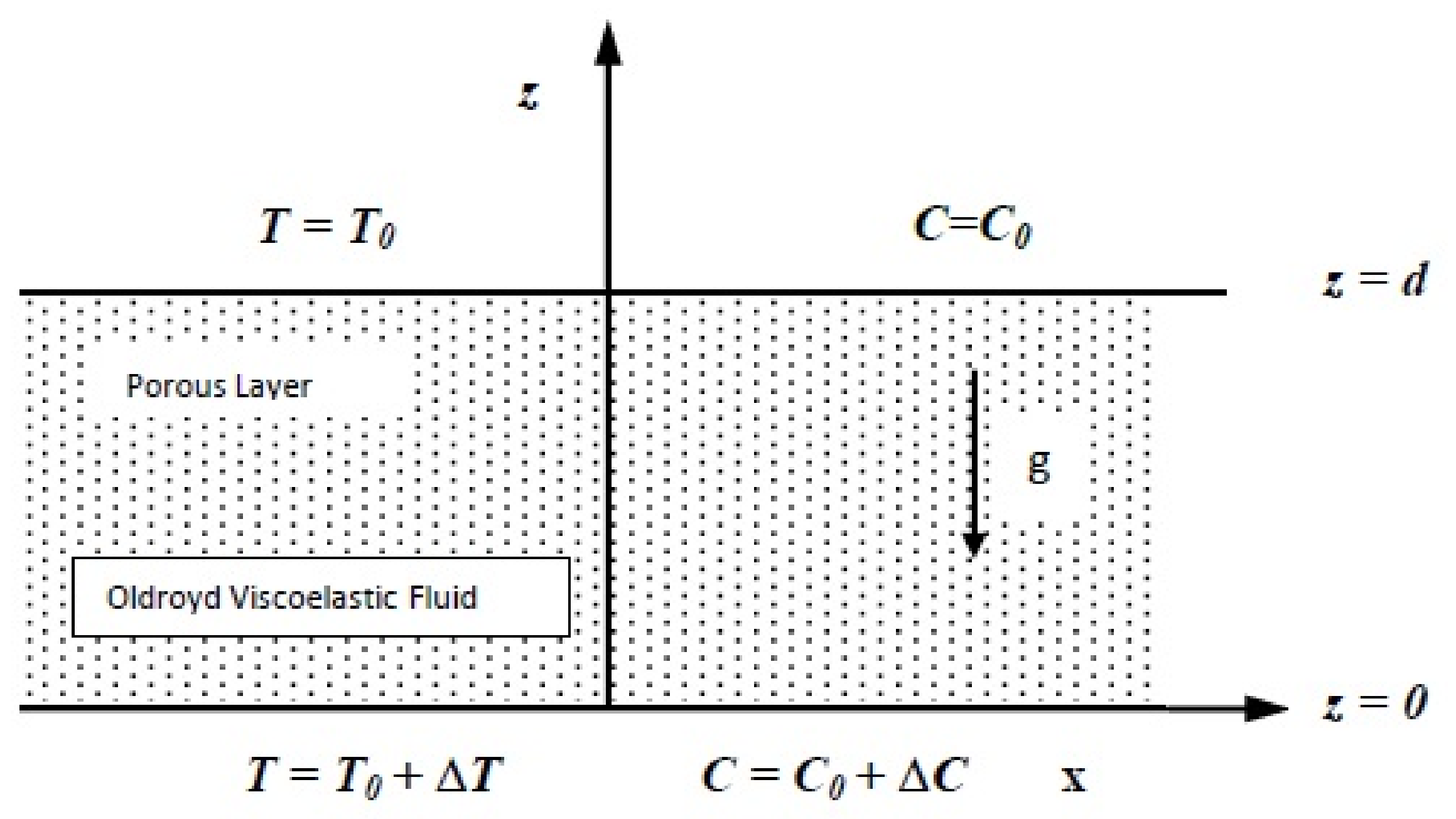
The physical model under consideration is a viscoelastic fluid saturated horizontal isotropic porous layer with an internal heat source, confined between two parallel horizontal planes at and with a distance d apart. A Cartesian frame of reference is chosen in such a way that the origin lies on the lower plane and the z-axis as vertically upward, where the gravity force is acting vertically downward. Adverse temperature and concentration gradients are applied across the porous layer, and the lower and upper planes are kept at temperature , concentration , and , respectively, where and are temperature difference and concentration difference between walls, respectively, as shown in Figure 1. In the momentum equation, the modified Darcy law has been applied for an Oldroyd type viscoelastic fluid. Both Soret and Dufour terms take to account in the temperature and concentration equations. In addition, the internal heat source parameter is involved in the temperature equation. Finally, the Oberbeck–Boussinesq approximation has been applied to account for the effect of density variations. Under these assumptions, the governing equations are given as [23]:
subject to the following boundary conditions:
where is the relaxation time parameter, is the retardation time parameter, is velocity , is the dynamic viscosity, Q is the internal heat source, K is the permeability, is the thermal diffusivity, T is temperature, is the thermal expansion coefficient, is the concentration expansion coefficient, is the concentration diffusivity of the fluid, is the ratio of heat capacities, and are the cross diffusion due to C and T components, respectively, is the density, is gravitational acceleration, and is the reference density, for the viscoelastic fluid of Oldroyd type . When , the Maxwell viscoelastic model is recovered. When , it reduces to a Newtonian fluid.
2.1. Basic State
Now, for the basic state, the fluid layer is stable and assumed to be quiescent. Therefore it has no motion and the velocity vector is set equal to zero, where the heat and mass are transferred by conduction only. Thus, the basic state is given by:
Substituting Equation (8) into Equations (1)–(4), we obtain:
where b refers to the basic state. The basic state temperature and concentration satisfy Equations (10) and (11) with boundary conditions at , and at .
By solving the resulted equations, the conduction state solution is obtained, and is given by:
where . Equations (12) and (13) represent the heat and mass transfer in conduction state only, where the layer is stable. This means no motion or convection exist in the layer and the transferred heat and mass occur by conduction only.
2.2. Perturbed State
Now, to study the stability of the system, we superimpose the infinitesimal perturbations on the basic state. Thus, the basic state is perturbed with thermal perturbation as follows:
where the primes denote that the quantities are infinitesimal perturbations. Now, we substitute Equation (14) into Equations (1)–(5), and using basic state Equations (9)–(11) we obtain:
Eliminate the pressure from Equation (16) by operating the curl twice to obtain:
Now, introduce the stream function , and use the following transformation:
into Equations (15), (17)–(19); we obtain:
where is the Vadasz number, is the Darcy number, is the Prandtl number, the thermal Rayleigh number, is the concentration Rayleigh number, is the internal Rayleigh number, is the kinematic viscosity, is the Lewis number, is the Soret parameter, is the Defour parameter, is the relaxation parameter, and is the retardation parameter; and . and are given in dimensionless form as:
where .
The viscoelastic character depends on the relaxation time parameter and the retardation time parameter , where these two parameters give the viscoelastic fluid its viscosity and elasticity. The smaller the relaxation parameter, the more fluid the material appears. is of order one for most viscoelastic fluids. For some special cases, is most likely in the range and is in the range for a diluted polymeric solution. At present, there are no experimental data for the ranges of the parameters, and hence a wide range of parameters were considered. Some parameters, such as and , depend on the fluid properties [43].
Now, Equations (21)–(23) are solved for stress free, isothermal, and isohaline scenarios. Therefore the boundary conditions are expressed as:
For the next steps the asterisks are removed, and and are set equal to unity for simplicity.
3. Linear Stability Theory
Stability means stability with respect to all infinitesimal disturbances. Thus, the reaction of the system with all disturbances should be examined. This can be established by considering an arbitrary disturbance as a superposition of certain basic possible modes and testing the stability of the system with all of these modes [44]. In the present problem, an arbitrary disturbance in terms of periodic waves will be analyzed. Therefore we assume the solution to be periodic waves as given in Equation (27).
In this section, the linear stability analysis is discussed. The thresholds of marginal and oscillatory convection are predicted. Equations (21)–(23) form an eigenvalue problem subjected to the boundary conditions given in Equation (26). For the onset of convection, the nonlinear terms in Equations (21)–(23) must be ignored and the resulting linear system is sufficient to study the onset of convection. Thus, to make the linear stability study, we neglect the nonlinear terms in Equations (21)–(23), and assume the solutions to be periodic waves of the form:
where () are the amplitudes of (), respectively. is a growth rate and in general a complex quantity and is a horizontal wave number. is the wave number that corresponds to disturbances. The reaction of the system to a disturbance can be studied in terms of system reaction to all disturbances of all associated wave numbers . This means that the stability will depend on its stability as a result of disturbances of all wave numbers and instability will follow from its instability as a result of disturbances of even one wave number. The infinitesimal perturbations may grow or damp depending on the values of the growth rate . Now, substitute Equation (27) into the linearized form of Equations (21)–(23) to obtain:
where . Now, change Equations (28)–(30) to a matrix form:
where:
For the non-trivial solution of Equation (31), the determinant must equal to zero, which implies an expression of the thermal Rayleigh number, and is given by:
where .
3.1. Marginal Stationary State
The growth rate sigma in general is a complex quantity and is given as . For (), the system is stable, and for , the system is unstable. For the existence of marginal curves (stationary or oscillatory) or neutral stability curves, the real part of sigma must be zero . Now, for the existence of a marginal stationary state the imaginary part must also equal zero . As a result, sigma becomes equal to zero [32]. Now, for the stationary Rayleigh number, substitute into Equation (32). Then, the stationary Rayleigh number is given as:
where .
It is noticeable that the expression of the stationary Rayleigh number that appears in Equation (33) is independent of the viscoelastic parameters, the relaxation time parameter and the retardation time parameter , where these two parameters give the viscoelastic fluid its viscosity and elasticity. Thus, when these two parameters do not appear in the expression of the stationary Rayleigh number, it means that the onset of convection via the stationary state will not be affected by these parameters. Therefore, the present fluid layer behaves as a Newtonian binary fluid layer. This is because the fluid in the base state has no flow and the viscoelasticity will not affect the onset of stationary convection when the flow is steady and weak.
Now, in the case with no internal heat source, Equation (33) becomes:
which recovers the results obtained by Malashetty et al. [45].
When the cross diffusion effects and internal heat source are absent, the result by Malashetty et al. [23] is recovered, when an isotropic porous layer is considered. Thus, Equation (33) becomes:
For , we have , and have the critical value for , which recovers the results obtained by Horton and Rogers [1] and Lapwood [2] for a single component convection in a porous medium.
The critical Rayleigh number for steady state convection in the presence of an internal heat source, the Soret and Dufour effects, is calculated from Equation (33) with variations of the parameters.
3.2. Marginal Oscillatory State
For the existence of a marginal oscillatory state, the real part must equal zero , but the imaginary part does not equal zero . Thus, in Equation (32) we set and cleared up the complex quantities from the denominator to obtain:
where is not given here for brevity.
From the previous equation, it follows that gives a stationary convection and gives an oscillatory convection, which gives the dispersion relation of the form:
where:
Now, the convection sets in via oscillatory mode if . To find an oscillatory marginal solution, we use Equation (36). For the value of , Equation (37) is solved and substituted in Equation (36) for a marginal oscillatory convection. However, Equation (37) is quadratic in , which can give more than one positive real root for some fixed values of parameters. Thus, first we determine the number of solutions of Equation (37). If there are no positive solutions, then no oscillatory instability is possible. If there are two positive solutions, then the minimum (over ) of Equation (36) gives the oscillatory Rayleigh number with given by Equation (37).
4. A Weak Nonlinear Theory
The aim of the linear theory discussed in Section 3 is to determine the critical values of the thermal Rayleigh number below which the system is stable, and above which it is unstable. Thus, when the flow with the thermal Rayleigh number is grater than critical values , the linear stability analysis will not give any idea about the flow field and become invalid, which is reasonable, because the nonlinear terms were neglected from the governing equations in the linear study. Linear stability theory does not give any information about the convection amplitudes, which is necessary to study the heat and mass transfer process.
In this section, a nonlinear stability analysis will be used to study the nonlinear effect on the flow field. The nonlinear study is performed involving a truncated Fourier series representations for stream function, temperature, and concentration. Nonlinear analysis with two terms of double Fourier series is enough to understand the physical mechanism for the rate of heat and mass transfer and to give more representation for nonlinear terms in the mathematical model with less mathematical analysis. In addition, it will be a step forward toward the study and generalization of the full nonlinear problem. Additionally, it is to be noted that the effect of nonlinearity is to distort the temperature and concentration fields through the interaction of and T, and and S, respectively. As a result, a component of the form will be generated [42].
For simplicity, the case of two-dimensional rolls is considered, and thus all physical quantities are made as independent of y. By eliminating pressure from Equation (16), introducing the stream function , using the transformations given in Equation (20), and dropping the asterisks, Equations (15)–(18) become:
Now consider a minimal Fourier series with one term in the stream function and two terms in the temperature and concentration fields in order to obtain some effect of non-linearity as given below [32]:
where the amplitudes and are functions of time and are to be determined. Substituting Equations (41)–(43) into Equations (38)–(40) and equating the coefficients of like terms of the resulting equations, a system of nonlinear differential equations is obtained and is given as follows:
An analytical solution to the nonlinear system of autonomous differential equations is not suitable for the general time-dependent variables. A numerical solution for the nonlinear system of autonomous differential equations can be established. Then the amplitude functions , , , and can be determined. Therefore, the Nusselt number and Sherwood number can be obtained as functions of time.
The steady analysis is performed by setting the left-hand side of Equations (44)–(48) as equal to zero,
with the consideration that all of the amplitudes are constants, since they are independent of time for the steady-state solution. We write and in terms of using Equations (49)–(53), and substitute these into Equation (49), with to obtain:
where:
The required root of Equation (54) is:
4.1. Steady Heat and Mass Transport
Heat and mass transport appears as a one of the most important issues in convection in fluids. That is because the onset of convection, as the Rayleigh number is increased, is more readily detected by its effect on the heat and mass transfer. In the basic state, heat and mass transfer are given by conduction only.
If H and J are the rate of heat and mass transfer per unit area, respectively, then [32]:
where the angular bracket represents the horizontal average. Additionally,
Substituting Equations (42) and (43) into Equations (59) and (60), respectively, and using the results in Equations (57) and (58), we obtain:
where , is given in Appendix A, and are given in terms of as follows:
where:
5. Results and Discussion
In this study, a porous layer saturated with viscoelastic fluid of Oldroyd type that is heated and salted from below was considered. The combined effects of cross-diffusion and internal heat source on the onset of stationary and oscillatory convection, as well as on the heat and mass transfer, were investigated using linear stability theory based on a normal mode technique, and weak nonlinear theory based on minimal representation of a truncated double Fourier series, respectively. Different values of governing parameters were selected to study instabilities and the convection process.
Equations (33) and (36) represent the critical thermal Rayleigh number for stationary and oscillatory modes, respectively. The onset of convection was investigated by varying the values of the following governing parameters: . A comparison between these two modes was made to check whether the convection was initiated via the stationary or oscillatory mode. The results were presented graphically in terms of marginal stability curves, whereby the system is stable/unstable below/above the curve. In each case, the following parameter values were adopted: , whereby one parameter was varied at a time to study its effect on system stability.
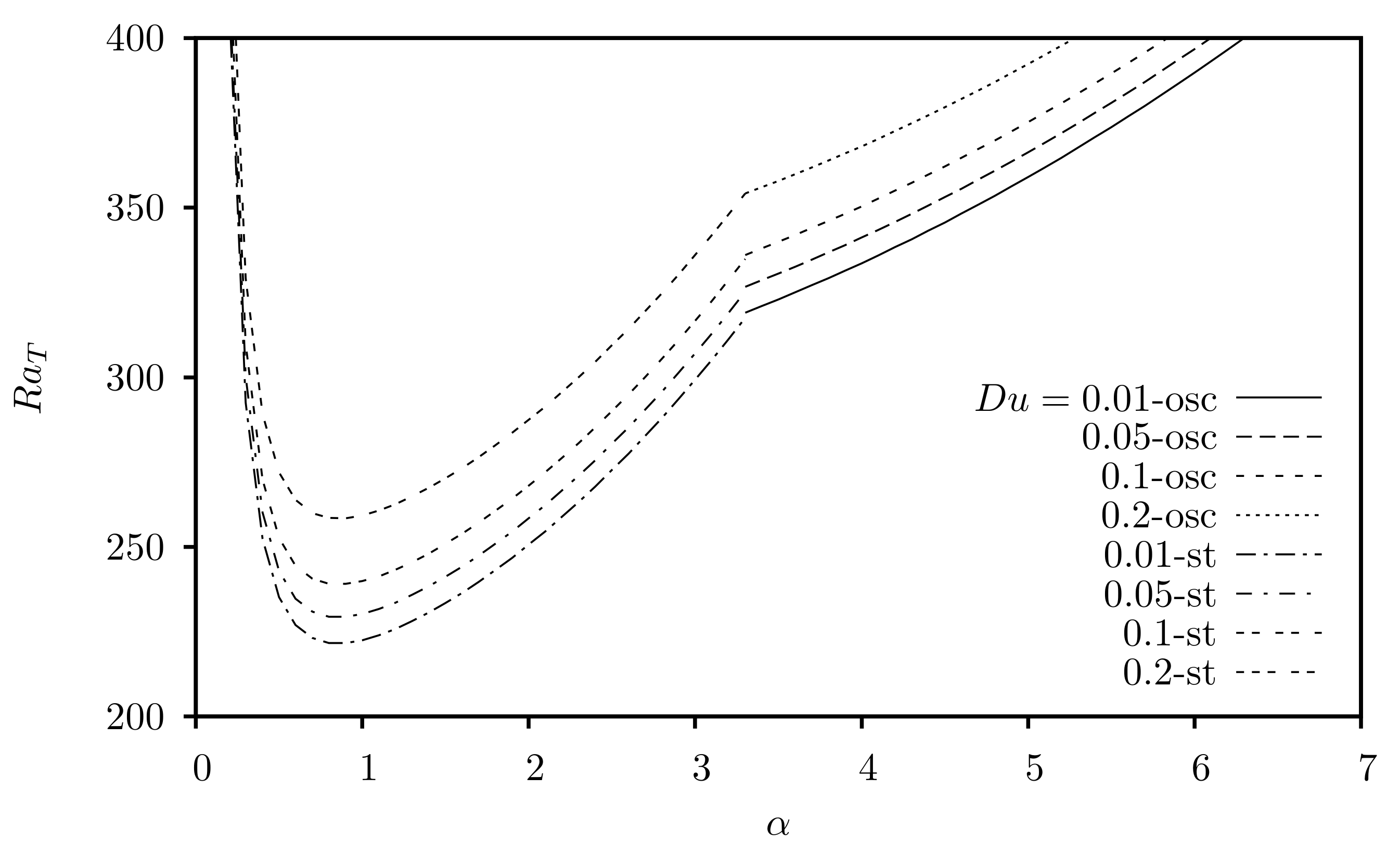
Figure 2 illustrates the effect of the Dufour parameter on the thermal Rayleigh number via stationary and oscillatory modes. Marginal stability curves showed that increases with the increase in . Moreover, as can be seen from the graph that in the oscillatory mode, an increase in increases the marginal curves as well as . Hence, the Dufour parameter has a stabilizing effect in both modes.
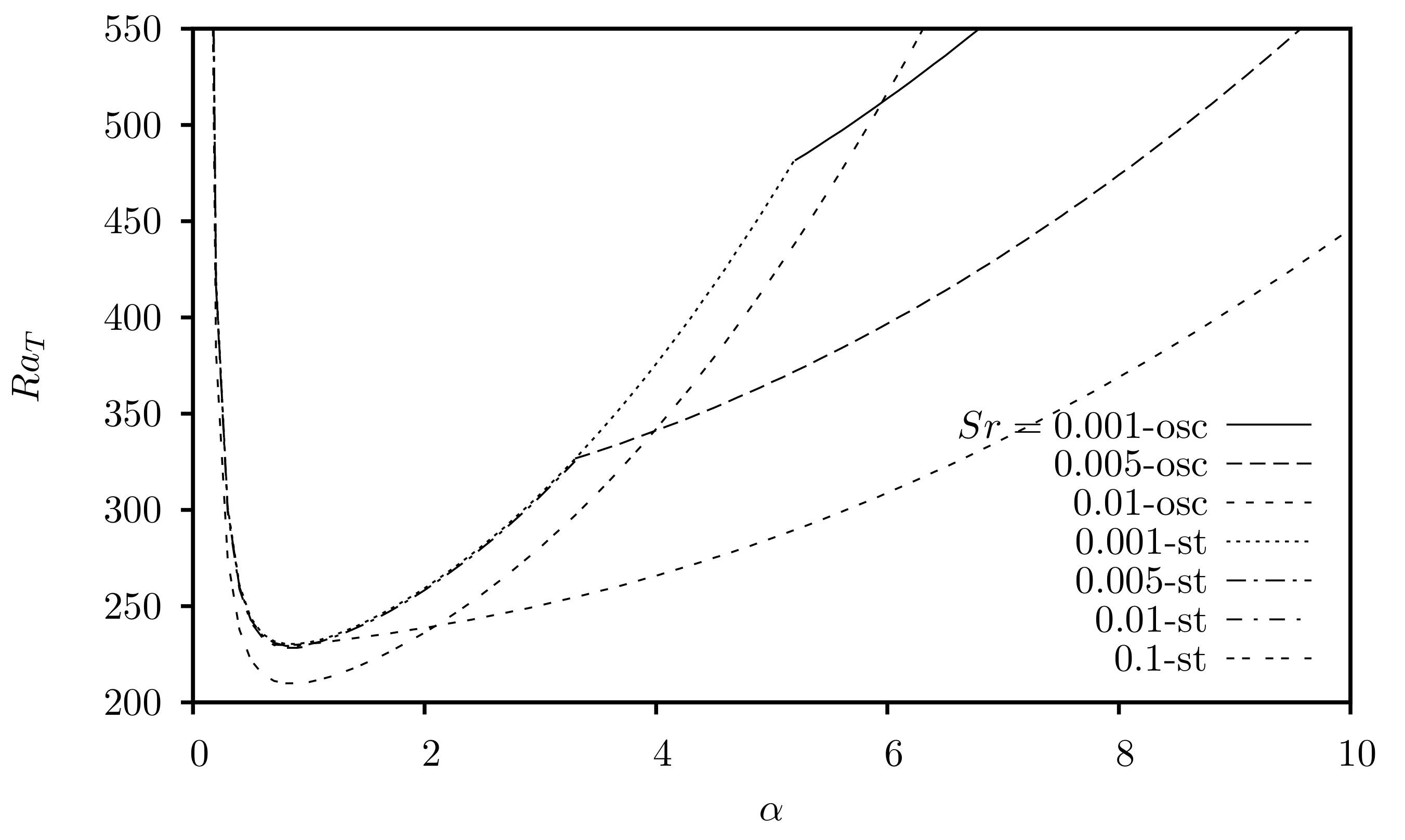
Figure 3 shows the effect of the Soret parameter on the stationary and oscillatory modes, indicating that an increase in decreases both the stationary marginal curves and . The Soret parameter also exerts a significant effect on the oscillatory convection. Specifically, as the value of increases, the critical thermal Rayleigh number decreases, indicating that the Soret parameter has a destabilizing effect on the system.
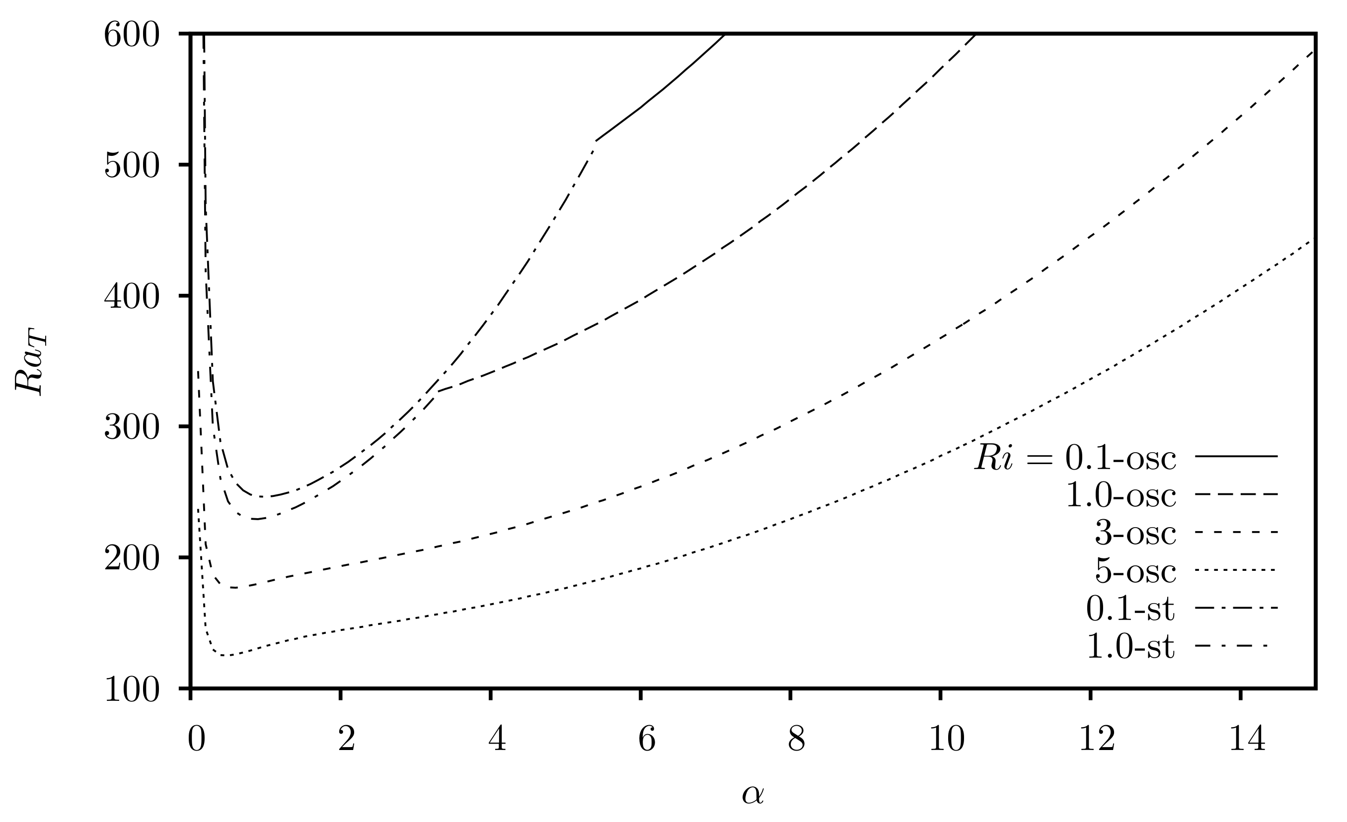
The effect of the internal Rayleigh number is presented in Figure 4. As can be seen from the graph, for smaller and greater values of , the convection is initiated via the stationary and oscillatory mode, respectively. In both modes, has a destabilizing effect.
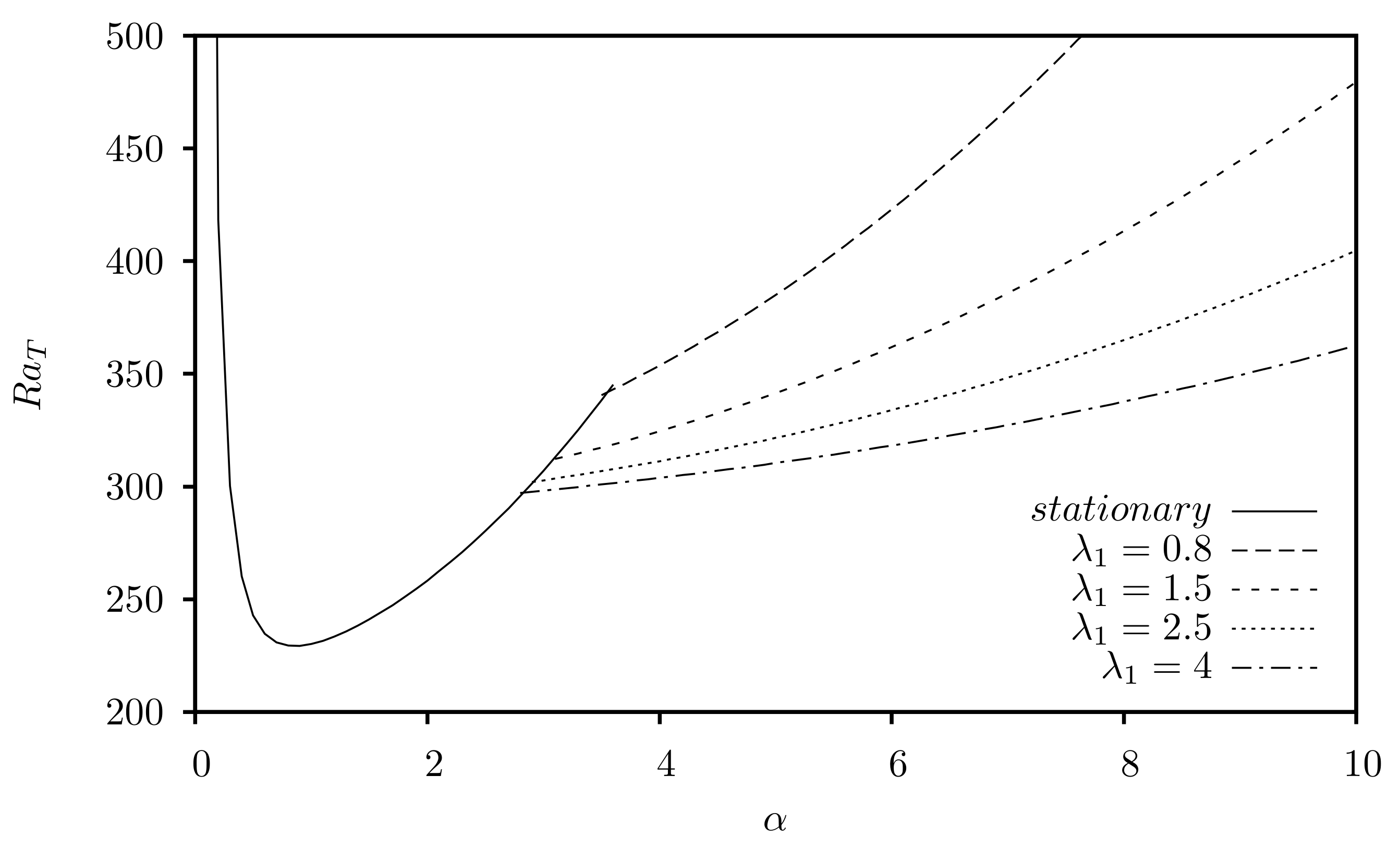
On the other hand, neither the relaxation time parameter nor the retardation time parameter affect the stationary thermal Rayleigh number, as indicated by Equation (33), which is independent of these two parameters. Nonetheless, a significant effect of and is observed on the onset of convection via the oscillatory mode. Figure 5 and Figure 6 illustrate the variation in in terms of and , respectively. As can be seen from these graphs, increasing decreases marginal curves, whereas an increase in increases both marginal curves and . Consequently, has a destabilizing and a stabilizing effect. It is noticeable that for , the marginal curves for oscillatory convection decrease in comparison with the Newtonian case . Therefore the system with is more unstable as compared to a Newtonian fluid.
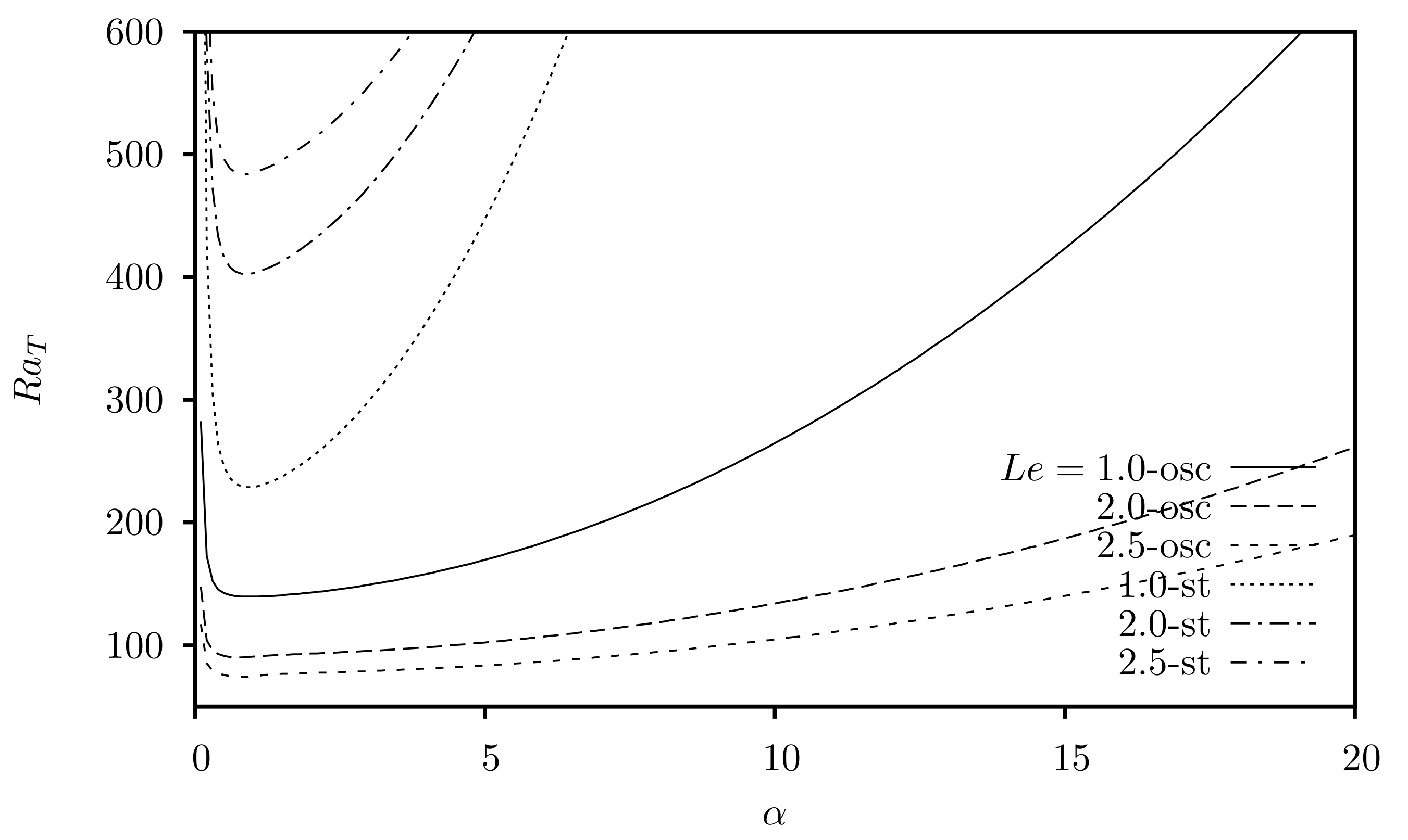
Figure 7 depicts the influence of the Lewis number on the onset of stationary and oscillatory convection, indicating that an increase in increases the marginal curves for the stationary mode, thus stabilizing the system. On the other hand, as an increasing has an opposite effect on the oscillatory convection, it destabilizes the system. This is because when , the heat diffusivity is higher than mass diffusivity. Thus, destabilizing the mass gradient enhances the onset of oscillatory convection.
The effect of the concentration Rayleigh number is depicted in Figure 8, indicating that, in both modes, an increase in increases the marginal curves as well as the thermal Rayleigh number. In addition, for , the convection is initiated via the oscillatory mode, whereas the stationary mode applies to higher values.
Figure 9, Figure 10, Figure 11, Figure 12, Figure 13, Figure 14, Figure 15 and Figure 16 depict the effects of all aforementioned governing parameters on the steady heat and mass transfer processes. In each case, one of the parameters varies and the others are set to the following values: . The parameters , and are not considered in the steady heat and mass transport, since the expressions for the Nusselt number and Sherwood number given in Equations (61) and (62) are independent of these parameters. In extant literature, heat and mass transfer have been studied in terms of the Nusselt number and Sherwood number, respectively. The findings yielded indicate that variation in and with the thermal Rayleigh number represents the convection when , which is the main concept behind the nonlinear stability theory indicating that the system is unstable.
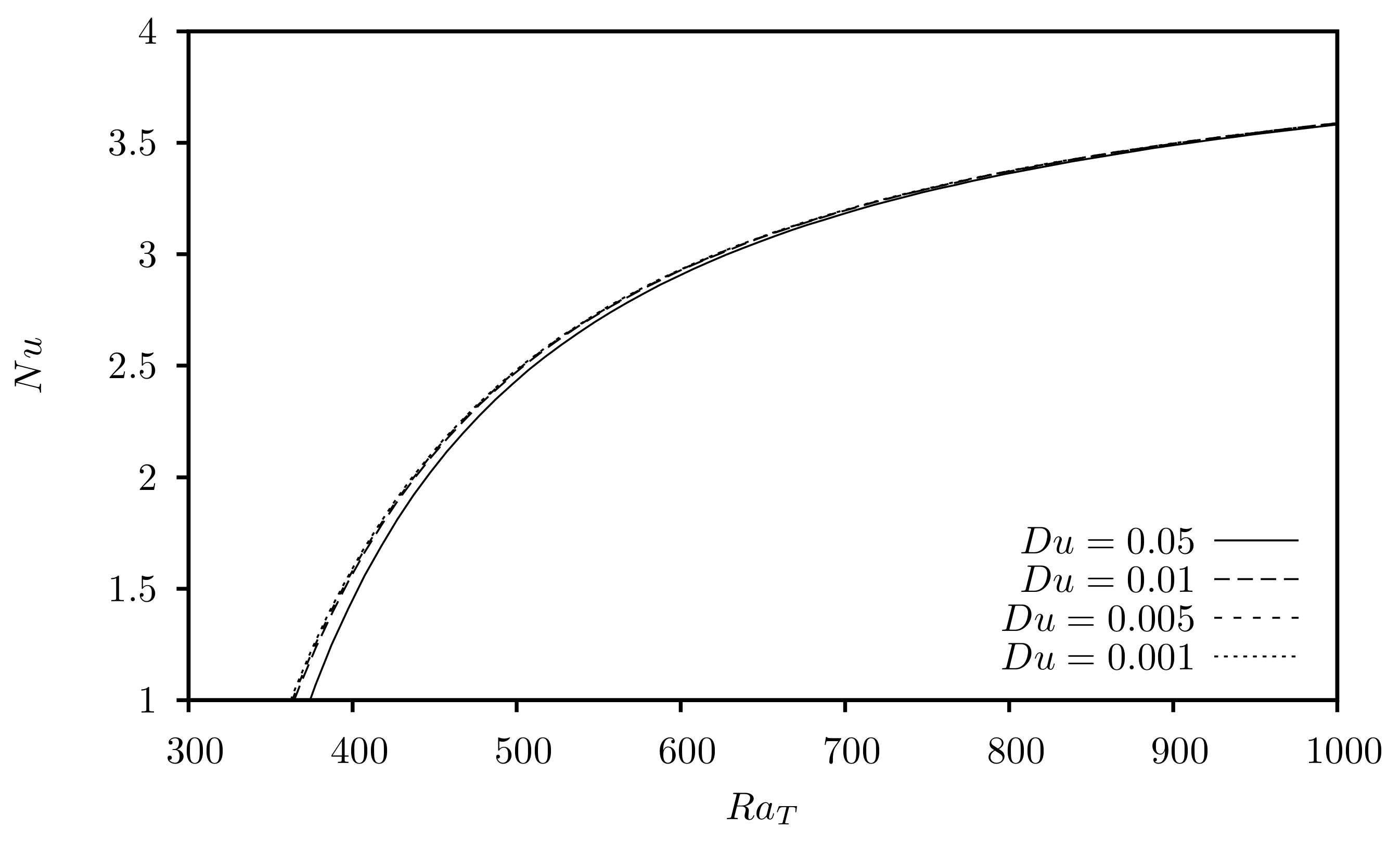
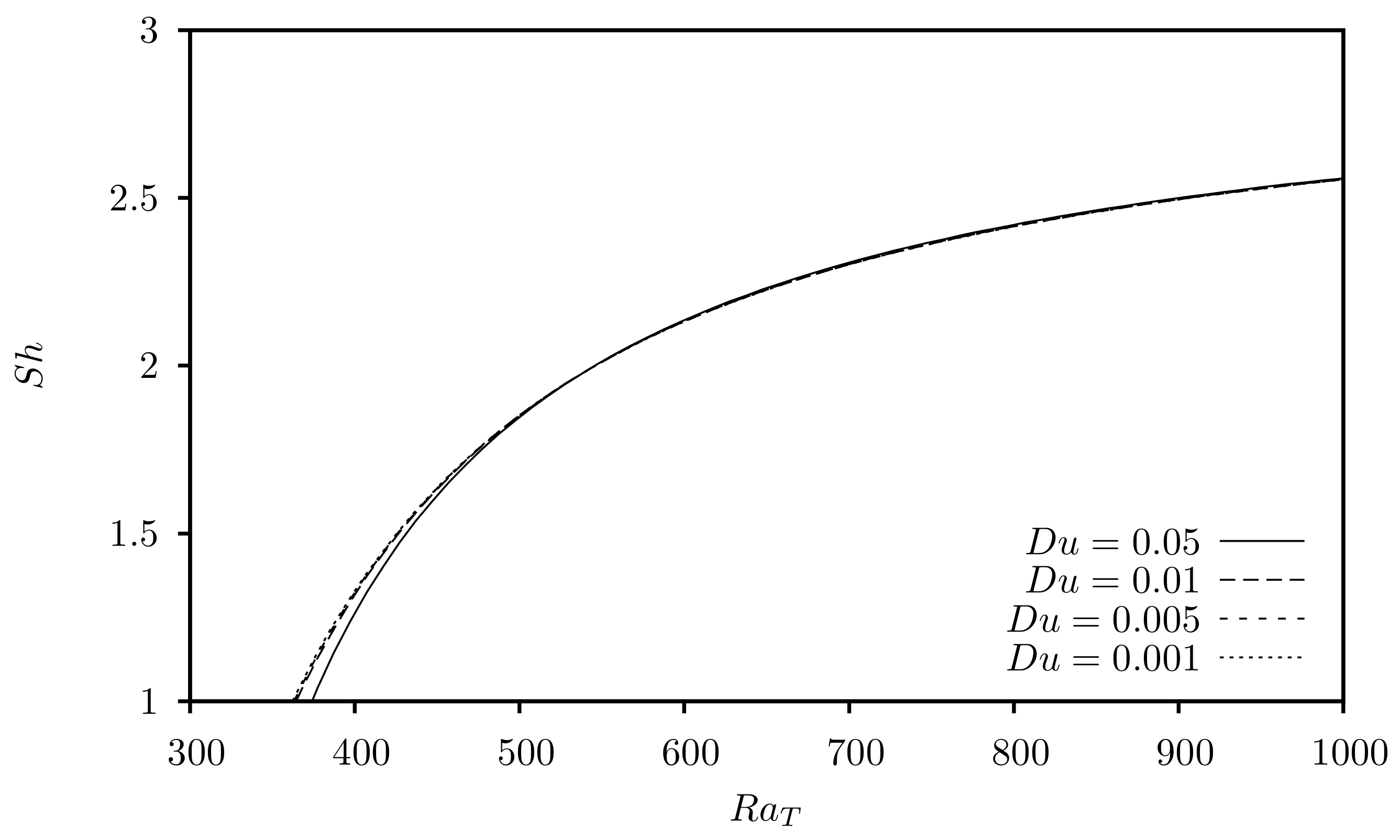
Figure 9, Figure 10, Figure 11 and Figure 12 illustrate the effect of all of the studied parameters on the heat transfer process in terms of the Nusselt number, and Figure 9 illustrates the effect of the Dufour parameter. It is evident that variation in does not exert a significant effect on the heat transfer process. However, as increases, a small decrease in can be noted.
Figure 10 depicts the influence of on heat transfer, indicating that an increase in increases , due to which heat transfer is enhanced. However, it is worth noting that, for , the effect of becomes insignificant even though continues to decline.
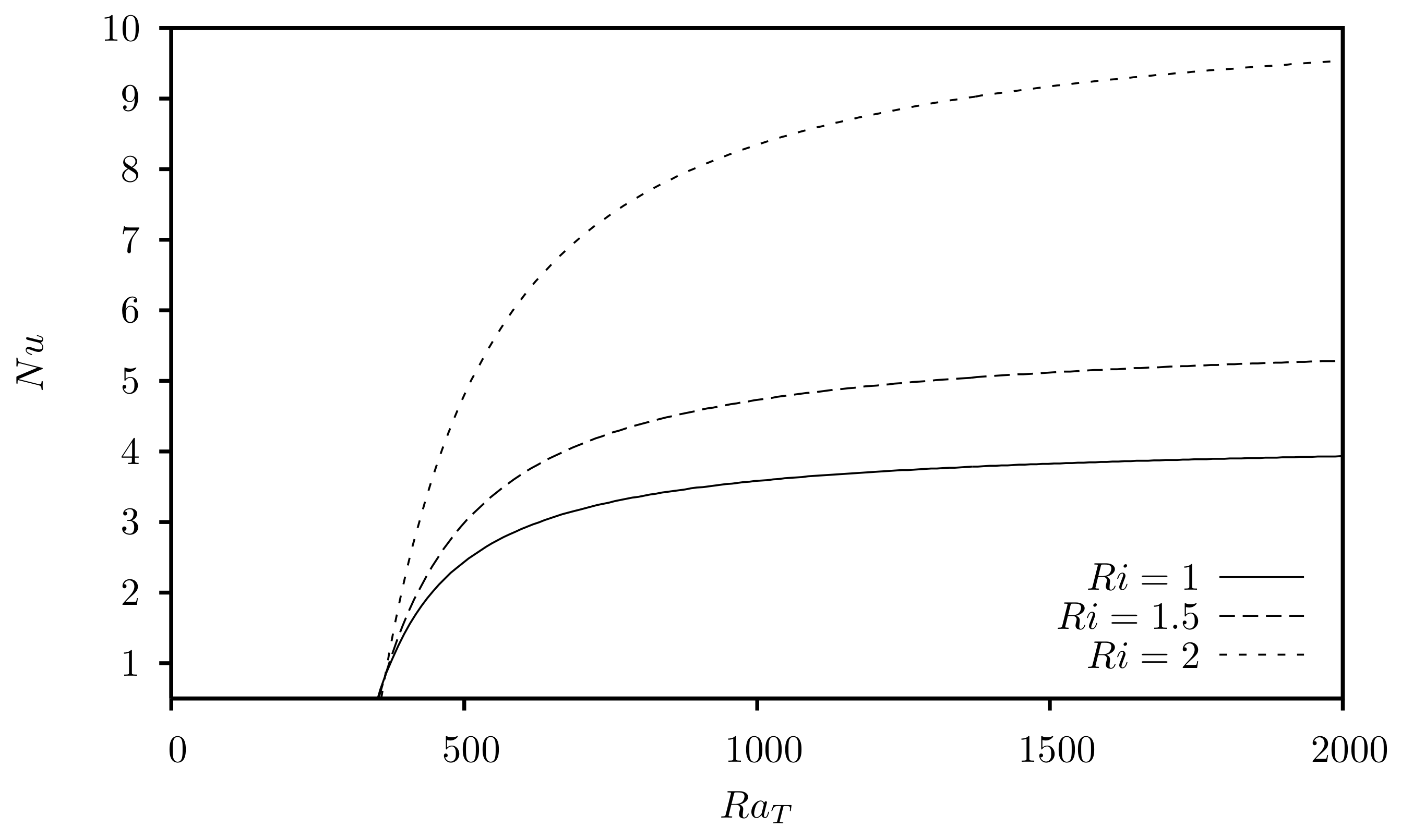
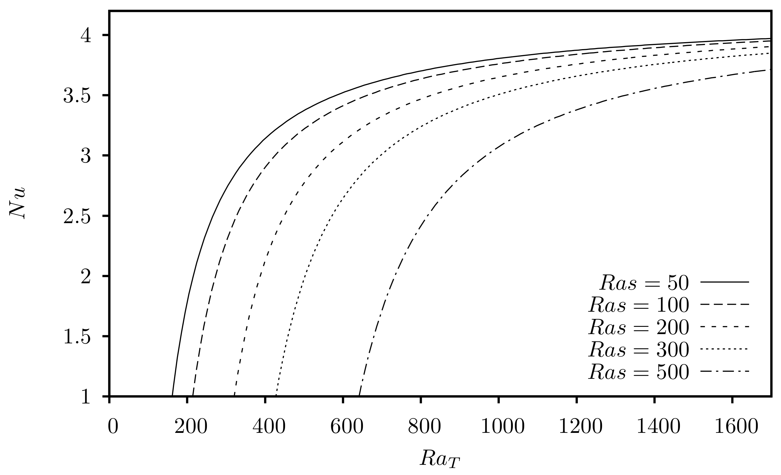
The effect of the internal Rayleigh number is illustrated in Figure 11, indicating that exerts a considerable influence on the heat transfer, as its increase increases and hence enhances the heat transfer process. The effect of is depicted in Figure 12, demonstrating that heat transfer is suppressed as values increase.
The influence of all aforementioned governing parameters on the mass transfer process is depicted in Figure 13, Figure 14, Figure 15 and Figure 16. The results are presented graphically in terms of the Sherwood number . Specifically, Figure 13 shows that variation in has a minimal effect on even though the critical thermal Rayleigh number increases as increases, which in turn decreases .
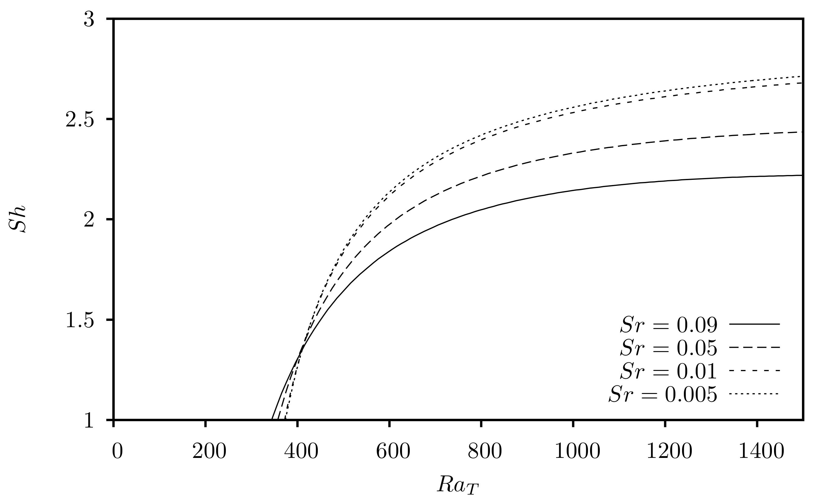
Figure 14 illustrates variations in as a result of changes in . It can be seen that, for , increases as increases, which in turn enhances mass transfer. Conversely, for , increasing decreases and thus suppresses mass transfer.
The influence of the internal Rayleigh number on the Sherwood number is depicted in Figure 15. Two regimes in the mass transfer process can be observed. Specifically, below a critical value, increasing decreases and hence suppresses mass transfer, while at above this value increasing increases and thus enhances mass transfer.
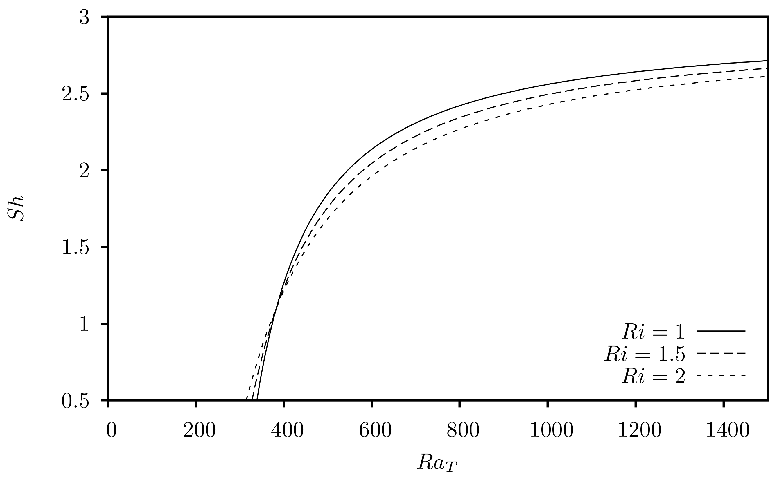
Figure 16 presents the effect of on , revealing that increasing decreases , which in turn suppresses the mass transfer process. When is increased beyond , a sharp increas in the values of the Nusselt number and the Sherwood number is observed. However, when continuing to increase , the change in Nu and Sh becomes insignificant.
6. Conclusions
The combined effect of an internal heat source and cross diffusion on double-diffusive convection in a viscoelastic fluid-saturated porous layer was studied analytically using linear and nonlinear stability analysis. The porous layer is heated and salted from below. In each case, the following parameter values were adopted: whereby one parameter was varied at a time to study its effect on system stability. For the stationary and oscillatory modes, it was found that increasing the values of the Dufour parameter , retardation time parameter , Lewis number , and concentration Rayleigh number stabilizes the system. On the other hand, increasing the values of the Soret parameter , internal Rayleigh number , and relaxation time parameter destabilize the system. Steady heat and mass transport are independent of both the relaxation time parameter and retardation time parameter . The effects of the Dufour parameter and concentration Rayleigh number are to suppress the heat and mass transfer processes as they increase. For high values of the thermal Rayleigh number , the effect of becomes insignificant. However, a small decrease in is still noticeable as increases. Increasing the internal Rayleigh number increases the Nusselt number as well as the heat transfer. On the other hand, there is a critical value for the thermal Rayleigh number , below which increasing the internal Rayleigh number decreases the Sherwood number and above which increasing the internal Rayleigh number increases the Sherwood number . Additionally, there is a critical value for the thermal Rayleigh number , where below this value the heat and mass transfer are enhanced as the Soret parameter increased, while above it they are suppressed.
Funding
The author is gratefully acknowledged the Scientific Research Council at Philadelphia University for funding the APC of this article.
Acknowledgments
Also, I would like to thank the reviewers for their valuable comments which enhanced the quality of the manuscript.
Conflicts of Interest
The author declares no conflict of interest.
Abbreviations
The following abbreviations are used in this manuscript:
| st | stationary |
| osc | oscillatory |
| c | critical |
| b | basic state |
Appendix A
References
- Horton, C.W.; Rogers, F.T. Convection currents in a porous medium. J. Appl. Phys. 1945, 16, 367–370. [Google Scholar] [CrossRef]
- Lapwood, E.R. Convection of a fluid in a porous medium. Proc. Camb. Philos. Soc. 1948, 44, 508–521. [Google Scholar] [CrossRef]
- Elder, J. Steady free convection in a porous medium heated from below. J. Fluid Mech. 1967, 27, 29–48. [Google Scholar] [CrossRef]
- Katto, Y.; Masuoka, T. Criterion for the onset of convective flow in a fluid in a porous medium. Int. J. Heat Mass Transf. 1967, 10, 297–309. [Google Scholar] [CrossRef]
- Ingham, D.B.; Pop, I. Transport Phenomena in Porous Media; Pergamon: Oxford, UK, 2005; Volume III. [Google Scholar]
- Vafai, K. Handbook of Porous Media, 2nd ed.; Taylor & Francis Group LLC: Abingdon, UK, 2005. [Google Scholar]
- Nield, D.A.; Bejan, A. Convection in Porous Media, 3rd ed.; Springer: New York, NY, USA, 2006. [Google Scholar]
- Gershuni, G.Z.; Zhukhovitskii, E.M.; Iurkov, I.S. On convective stability in the presence of periodically varying parameter. J. Fluid Mech. 1970, 34, 442–452. [Google Scholar] [CrossRef]
- Gresho, P.M.; Sani, R.L. The effects of gravity modulation on the stability of a heated fluid layer. J. Fluid Mech. 1970, 40, 783–806. [Google Scholar] [CrossRef]
- Malashetty, M.S.; Padmavathi, V. Effect of gravity modulation on the onset of convection in a fluid and porous layer. Int. J. Eng. Sci. 1997, 35, 829–840. [Google Scholar] [CrossRef]
- Abidi, A.; Raiza, Z.; Madiouli, J. Magnetic field effect on the double diffusive natural convection in three-dimensional cavity filled with micropolar nanofluid. Appl. Sci. 2018, 8, 2342. [Google Scholar] [CrossRef] [Green Version]
- Kumar, A.; Gupta, V.K.; Maena, N.; Hashim, I. Effect of rotational speed modulation on the weakly nonlinear heat transfer in Walter-B viscoelastic fluid in the highly permeable porous medium. Mathematics 2020, 8, 1448. [Google Scholar] [CrossRef]
- Maleki, H.; Safaei, M.R.; Alrashed, A.A.A.A.; Kasaeian, A. Flow and heat transfer in non-Newtonian nanofluids over porous surfaces. J. Therm. Anal. Calorim. 2019, 135, 1655–1666. [Google Scholar] [CrossRef]
- Govender, S. Linear stability and convection in a gravity modulated porous layer heated from below: Transition from synchronous to subharmonic solutions. Trans. Porous Media 2005, 59, 227–238. [Google Scholar] [CrossRef]
- Saravanan, S.; Purusothaman, A. Floquet instability of a modulated Rayleigh-Benard problem in an anisotropic porous medium. Int. J. Therm. Sci. 2009, 48, 2085–2091. [Google Scholar] [CrossRef]
- Srivastava, A.K.; Bhadauria, B.S. Linear stability of solutal convection in a mushy layer subjected to gravity modulation. Commun. Nonlinear Sci. Numer. Simulat. 2011, 16, 3548–3558. [Google Scholar] [CrossRef]
- Govender, S. On the effect of anisotropy on the stability of convection in rotating porous media. Trans. Porous Media 2006, 64, 413–422. [Google Scholar] [CrossRef]
- Malashetty, M.S.; Swamy, M. Effect of rotation on the onset of thermal convection in a sparsely packed porous layer using a thermal non-equilibrium model. Int. J. Heat Mass Transf. 2010, 53, 3088–3101. [Google Scholar] [CrossRef]
- Maleki, H.; Alsarraf, J.; Moghanizadeh, A.; Hajabdollahi, H.; Safaei, M.R. Heat transfer and nanofluid flow over a porous plate with radiation and slip boundary conditions. J. Cent. South Univ. 2019, 26, 1099–1115. [Google Scholar] [CrossRef]
- Herbert, D.M. On the stability of viscoelastic liquids in heated plane Couette flow. J. Fluid Mech. 1963, 17, 353–359. [Google Scholar] [CrossRef]
- Green, T. Oscillating convection in an elasticoviscous liquid. Phys. Fluids 1968, 11, 1410. [Google Scholar] [CrossRef]
- Kim, M.C.; Lee, S.B.; Kim, S.; Chung, B.J. Thermal instability of viscoelastic fluids in porous media. Int. J. Heat Mass Transf. 2003, 46, 5065–5072. [Google Scholar] [CrossRef]
- Malashetty, M.S.; Tan, W.C.; Swamy, M. The onset of double diffusive convection in a binary viscoelastic fluid saturated anisotropic porous layer. Phys. Fluids 2009, 21, 084101. [Google Scholar] [CrossRef]
- Narayana, M.; Sibanda, P.; Siddheshwar, P.G.; Jayalatha, G. Linear and nonlinear stability analysis of binary viscoelastic fluid convection. App. Math. Model. 2013, 37, 8162–8178. [Google Scholar] [CrossRef] [Green Version]
- Bhadauria, B.S.; Kiran, P. Weakly nonlinear oscillatory convection in a viscoelastic fluid saturating porous medium under temperature modulation. Int. J. Heat Mass Transf. 2014, 77, 843–851. [Google Scholar] [CrossRef]
- Altawallbeh, A.A.; Hashim, I.; Tawalbeh, A.A. Thermal non-equilibrium double diffusive convection in a Maxwell fluid with internal heat source. J. Phys. 2018, 1132, 012027. [Google Scholar] [CrossRef]
- Awad, F.G.; Sibanda, P.; Motsa, S.S. On the linear stability analysis of a Maxwell fluid with double-diffusive convection. Appl. Math. Model. 2010, 34, 3509–3517. [Google Scholar] [CrossRef]
- Wang, S.; Tan, W. Stability analysis of soret-driven double-diffusive convection of Maxwell fluid in a porous medium. Int. J. Heat Fluid Flow 2011, 32, 88–94. [Google Scholar] [CrossRef]
- Zhao, M.; Wang, S.; Zhang, Q. Onset of triply diffusive convection in a Maxwell fluid saturated porous layer. Appl. Math. Model. 2014, 38, 2345–2352. [Google Scholar] [CrossRef]
- Parthiban, C.; Parthiban, P.R. Thermal instability in an anisotropic porous medium with internal heat source and inclined temperature gradient. Int. Commun. Heat Mass Transf. 1997, 24, 1049–1058. [Google Scholar] [CrossRef]
- Bhadauria, B.S. Double-Diffusive Convection in a Saturated Anisotropic Porous Layer with Internal Heat Source. Transp. Porous Media 2012, 92, 299–320. [Google Scholar] [CrossRef]
- Altawallbeh, A.A.; Bhadauria, B.S.; Hashim, I. Linear and nonlinear double-diffusive convection in a saturated anisotropic porous layer with Soret effect and internal heat source. Int. J. Heat Mass Transf. 2013, 59, 103–111. [Google Scholar] [CrossRef]
- Badruddin, I.A. Numerical Analysis of thermal non-equilibrium in porous medium subjected to internal heating. Mathematics 2019, 7, 1085. [Google Scholar] [CrossRef] [Green Version]
- Altawallbeh, A.A.; Hashim, I.; Bhadauria, B.S. Magneto-double diffusive convection in a viscoelastic fluid saturated porous layer with internal heat source. AIP Conf. Proc. 2019, 2116, 030015. [Google Scholar]
- Rana, P.; Khurana, M. LTNE thermoconvective instability in Newtonian rotating layer under magnetic field utilizing nanoparticles. J. Therm. Anal. Calorim. 2020. [Google Scholar] [CrossRef]
- Storesletten, L.; Rees, D.A.S. Onset of Convection in an Inclined Anisotropic Porous Layer with Internal Heat Generation. Fluids 2019, 4, 75. [Google Scholar] [CrossRef] [Green Version]
- Maleki, H.; Safaei, M.R.; Togun, H.; Dahari, M. Heat transfer and fluid flow of pseudo-plastic nanofluid over a moving permeable plate with viscous dissipation and heat absorption/generation. J. Therm. Anal. Calorim. 2019, 135, 1643–1654. [Google Scholar] [CrossRef]
- Taslim, M.E.; Narusawa, U. Binary fluid convection and double diffusive convection in porous medium. J. Heat Mass Transf. 1986, 108, 221–224. [Google Scholar] [CrossRef]
- Rudraiah, N.; Siddheshwar, P.G. A weak nonlinear stability analysis of double diffusive convection with cross-diffusion in a fluid saturated porous medium. Heat Mass Transf. 1998, 33, 287–293. [Google Scholar] [CrossRef] [Green Version]
- Gaikwad, S.N.; Malashetty, M.S.; Rama Parasad, K. Linear and non-linear double diffusive convection in a fluid-saturated anisotropic porous layer with cross-diffusion effects. Transp. Porous Media 2009, 80, 537–560. [Google Scholar] [CrossRef]
- Malashetty, M.S.; Pop, I.; Kollur, P.; Sidrama, W. Soret effect on double diffusive convection in a Darcy porous medium saturated with a couple stress fluid. Int. J. Thermal Sci. 2011, 53, 130–140. [Google Scholar] [CrossRef]
- Altawallbeh, A.A.; Bhadauria, B.S.; Hashim, I. Linear and nonlinear double-diffusive convection in a saturated porous layer with Soret effect under local thermal non-equilibrium model. J. Porous Media 2018, 21, 1395–1413. [Google Scholar] [CrossRef]
- Malashetty, M.S.; Swamy, M. The onset of double diffusive convection in a viscoelastic fluid layer. J. Non-Newtonian Fluid Mech. 2010, 165, 1129–1138. [Google Scholar] [CrossRef]
- Chandrasekhar, S. Hydrodynamic and Hydromagnetic Stability; Dover: New York, NY, USA, 1981. [Google Scholar]
- Malashetty, M.S.; Bharati, S. Biradar The onset of double diffusive convection in a binary Maxwell fluid saturated porous layer with cross diffusion effects. Phys. Fluids 2011, 23, 064109. [Google Scholar] [CrossRef]
Figure 1.
Physical configuration of the problem.

Figure 2.
Effect of on the marginal stability curves for stationary and oscillatory convection with respect to the wave number .
Figure 2.
Effect of on the marginal stability curves for stationary and oscillatory convection with respect to the wave number .

Figure 3.
Effect of on the marginal stability curves for stationary and oscillatory convection with respect to the wave number .
Figure 3.
Effect of on the marginal stability curves for stationary and oscillatory convection with respect to the wave number .

Figure 4.
Effect of on the marginal stability curves for stationary and oscillatory convection with respect to the wave number .
Figure 4.
Effect of on the marginal stability curves for stationary and oscillatory convection with respect to the wave number .

Figure 5.
Effect of on the marginal stability curves for oscillatory convection with respect to the wave number .
Figure 5.
Effect of on the marginal stability curves for oscillatory convection with respect to the wave number .

Figure 6.
Effect of on the marginal stability curves for oscillatory convection with respect to the wave number .
Figure 6.
Effect of on the marginal stability curves for oscillatory convection with respect to the wave number .

Figure 7.
Effect of on the marginal stability curves for stationary and oscillatory convection with respect to the wave number .
Figure 7.
Effect of on the marginal stability curves for stationary and oscillatory convection with respect to the wave number .

Figure 8.
Effect of on the marginal stability curves for stationary and oscillatory convection with respect to the wave number .
Figure 8.
Effect of on the marginal stability curves for stationary and oscillatory convection with respect to the wave number .

Figure 9.
Variation of with for steady nonlinear stability: effect of for , .

Figure 10.
Variation of with for steady nonlinear stability: effect of for , .

Figure 11.
Variation of with for steady nonlinear stability: effect of for , .

Figure 12.
Variation of with for steady nonlinear stability: effect of for , .

Figure 13.
Variation of with for steady nonlinear stability: effects of for .

Figure 14.
Variation of with for steady nonlinear stability: effects of for .

Figure 15.
Variation of with for steady nonlinear stability: effect of for .

Figure 16.
Variation of with for steady nonlinear stability: effect of for .

Publisher’s Note: MDPI stays neutral with regard to jurisdictional claims in published maps and institutional affiliations. |
© 2021 by the author. Licensee MDPI, Basel, Switzerland. This article is an open access article distributed under the terms and conditions of the Creative Commons Attribution (CC BY) license (https://creativecommons.org/licenses/by/4.0/).
Share and Cite
MDPI and ACS Style
Altawallbeh, A.A. Cross Diffusion Effect on Linear and Nonlinear Double Diffusive Convection in a Viscoelastic Fluid Saturated Porous Layer with Internal Heat Source. Fluids 2021, 6, 182. https://0-doi-org.brum.beds.ac.uk/10.3390/fluids6050182
AMA Style
Altawallbeh AA. Cross Diffusion Effect on Linear and Nonlinear Double Diffusive Convection in a Viscoelastic Fluid Saturated Porous Layer with Internal Heat Source. Fluids. 2021; 6(5):182. https://0-doi-org.brum.beds.ac.uk/10.3390/fluids6050182
Chicago/Turabian StyleAltawallbeh, A.A. 2021. "Cross Diffusion Effect on Linear and Nonlinear Double Diffusive Convection in a Viscoelastic Fluid Saturated Porous Layer with Internal Heat Source" Fluids 6, no. 5: 182. https://0-doi-org.brum.beds.ac.uk/10.3390/fluids6050182