
On the Use of Probability-Based Methods for Estimating the Aerodynamic Boundary-Layer Thickness
by
 ,
,
Andrey V. Boiko
1,*,† ,
,
Kirill V. Demyanko
1,2,†,
Yuri M. Nechepurenko
1,2,† and
Grigory V. Zasko
1,2,† 1
Khristianovich Institute of Theoretical and Applied Mechanics SB RAS, Institutskaya Str. 4/1, 630090 Novosibirsk, Russia
2
Marchuk Institute of Numerical Mathematics RAS, Gubkina Str. 8, 119333 Moscow, Russia
*
Author to whom correspondence should be addressed.
†
These authors contributed equally to this work.
Fluids 2021, 6(8), 267; https://0-doi-org.brum.beds.ac.uk/10.3390/fluids6080267
Submission received: 27 June 2021
/
Revised: 20 July 2021
/
Accepted: 23 July 2021
/
Published: 28 July 2021
(This article belongs to the Special Issue Stochastic Equations in Fluid Dynamics)
Abstract
:In this paper, known probabilistic methods for estimating the thickness of the boundary layer of a two-dimensional laminar flow of viscous incompressible fluid are extended to three-dimensional laminar flows of a viscous compressible medium. Their applicability to the problems of boundary-layer stability is studied with the software package, which allows us to compute the position of laminar-turbulent transition in three-dimensional aerodynamic configurations.
1. Introduction
In numerical studies of the stability of the laminar boundary layer to small disturbances, in order to determine the onset of transition to turbulence, all flow parameters outside the boundary layer are usually replaced by their values at the boundary-layer edge. This approach is justified by the order-of-magnitude analysis, when the curvature of the flow-exposed body is neglected. An overestimation of the boundary-layer thickness can lead to unnecessary computations due to the need to check for some ‘spurious’ instabilities, which are in fact unrelated to the transition in the boundary layer, while its underestimation can lead to a velocity distribution in the form of a broken curve that results in improper stability computations of the boundary layer. Thus, it is important to adequately estimate the proper boundary-layer thickness.
This paper is devoted to the development and analysis of a method for estimating the laminar-boundary-layer thickness proposed in [1,2]. The method is based on the probabilistic treatment of the problem, which arose from the observation that the second wall-normal derivative of laminar-flow velocity at a flat plate has a Gaussian-like profile, that allows a description of the boundary-layer thickness in terms of Gaussian-like core central moments. The probabilistic approach for estimating the boundary-layer thickness has been proposed and applied in the past only for two-dimensional (2D) flows of a viscous incompressible fluid. In this paper, we extend it to three-dimensional (3D) flows of compressible fluids.
For numerical experiments, we use the software package [3,4], which is designed to predict the onset of laminar-turbulent transition (LTT) in 3D aerodynamic boundary layers, using the data obtained with engineering precision by a gas-dynamic code. The main result of the software package is the distribution of so-called N-factors for Tollmien-Schlichting (TS) and crossflow (CF) instabilities in the boundary layer. The LTT onset is predicted by the method based on the N-factor distribution and values of the threshold N-factors (see, e.g., [5]). The software constructs two-dimensional slices perpendicular to the flow-exposed surface (wall) for 3D boundary layers. Then a physically justified method is applied for estimating the boundary-layer thickness in these slices using the distribution of stagnation enthalpy derived from Bernoulli’s equation for compressible media. The parameter of this method is an admissible relative deviation of the stagnation enthalpy from the stagnation enthalpy in the external flow. Numerous tests performed for different aerodynamic configurations have shown that, although the proper choice of the parameter depends on the configuration, the resulting boundary-layer thickness proves to be adequate for investigating the flow stability. It gives us a reference boundary-layer thickness to analyze the results of probabilistic approaches.
The structure of the paper is as follows. In Section 2, the construction of 2D slices in the wall-normal direction for a 3D boundary layer is outlined. Section 3 introduces the necessary notations and describes two methods for determining the boundary-layer thickness. The results of numerical experiments with flows in two typical three-dimensional aerodynamic configurations are presented in Section 4. The conclusions are summarized in Section 5.
2. Construction of 2D Slices
The construction of 2D non-planar boundary-layer slices along some disturbance propagation lines is a prerequisite for the stability analysis and the prediction of transition onset. There are several different approaches to construct such lines (see, e.g., [6,7,8,9,10,11]). However, experimental observations and numerical computations show that these lines are close to surface streamlines in the inviscid approximation [7,12,13].
In the present work, the algorithm described in detail in [4] is used for constructing the slices. It constructs some initial outward normal to the surface in the formed attached laminar boundary layer followed by a generation of a nonuniform grid along the normal with a refinement toward the surface, with flow data being interpolated onto the grid. Using the interpolated data, the boundary-layer thickness is determined by an analysis of the stagnation enthalpy in the boundary layer (Bernoulli’s equation for compressible fluid). The direction along the normal is taken as the local wall-normal direction, the component of the velocity vector at the boundary-layer edge perpendicular to the normal is taken as the local streamwise direction, and the direction orthogonal to the first two directions and forming a right coordinate system with them is taken as the local transverse direction. The data on the flow are presented in the local scaled coordinates x, y, z, where x is the streamwise coordinate (the length of the arc along the surface from the beginning of the slice to be constructed to the base of the normal), y is the wall-normal coordinate (the distance to the surface along the normal) and z is the transverse coordinate.
Then, the algorithm constructs the streamline upstream and downstream from a starting point (selected on the initial normal) by solving the corresponding system of ordinary differential equations with a fourth- or fifth-order Runge-Kutta method. A 2D boundary-layer slice is constructed along the resulting streamline: a uniform grid is selected on the streamline, a normal is lowered from each node of this grid to the surface, a grid is constructed on each normal, similar to the one that was constructed on the initial normal, and the parameters of the laminar flow are interpolated to this grid. Based on the analysis of the stagnation enthalpy, the boundary-layer edge is determined and a local orthonormal basis is constructed. The flow data are presented in the local coordinates. Only the flow data along the normals located in the region of the formed attached boundary layer are considered.
3. Methods for Determining the Proper Boundary-Layer Thickness
Let us consider a 2D slice of a 3D boundary layer and a fixed normal to the surface in this slice obtained according to Section 2 (see Figure 1 illustrating the slices for 3D configurations used in Section 4). As we consider spatially-varying quantities only on a fixed normal of the slice, the dependence on x and z is further omitted. Thus, y is the only spatial coordinate varying from 0 (the surface) to h (the height of the normal). We assume that the value of h is much greater than the boundary-layer thickness estimated by any known method. In what follows, , , and are the streamwise (along x), wall-normal (along y) and transverse (along z) velocity components, respectively; is the static pressure, is the density of the fluid, is the temperature, R is the specific gas constant, and is the adiabatic index.
3.1. Method Based on Bernoulli’s Equation
The main idea of this method follows from the observation that Bernoulli’s equation for incompressible laminar flows at constant temperature
is valid along an inviscid streamline where viscous forces can be neglected. Hence, Bernoulli’s equation holds far from the surface and does not hold in a boundary layer where the viscous forces are significant. A generalization of Bernoulli’s equation to compressible flows can be obtained from the Euler equation and thermodynamic relations [14]. For an isentropic flow in the absence of volumetric forces (gravity, etc.), it takes the form
where I is the specific enthalpy. For an ideal gas [14],
and therefore
The quantity H is called the stagnation enthalpy as it is equal to the specific enthalpy at the stagnation point [14]. Based on the stagnation enthalpy, the boundary-layer thickness along a given normal to the surface can be estimated as follows:
where is the parameter being chosen using an expert judgement for the flow under study.
3.2. Probability-Based Methods
The function , where U is the streamwise velocity component of a laminar flow of a viscous incompressible fluid over a flat plate, is similar to the Gaussian function. Based on this observation, a probabilistic approach was proposed in [1] for a mathematical description of boundary-layer characteristics. It was suggested to consider a random variable with the probability density function , where , with the following expected value and k-th central moments :
According to [1], is interpreted as the boundary-layer center, as its width, and as its edge (thickness), where is an adjustable constant.
It was noted in [2] that functions and , where is the displacement thickness, also have properties of the probability density function of a random variable. Based on this, the k-th central moments,
are introduced, where
Using these moments, the formulas and were proposed for the boundary-layer thickness, where and are adjustable constants. In [1,2] the use of the following constant values was encouraged: , , , but their change is allowed. In addition, it is implicitly assumed that is the maximum velocity of the flow, that is, .
For computing , and , it is necessary to differentiate numerically the main flow velocity that can lead to a significant error, especially when the velocity profile is obtained from physical experiments or engineering computations. To overcome this problem, it was proposed in [2] to compute the moments, using the auxiliary integrals,
which makes it possible to avoid the derivation of the main flow velocity and results in the following formulas:
for computing the proposed boundary-layer thicknesses ( is the displacement thickness). Note that in (2) completely getting rid of the numerical differentiation failed, as it is required to differentiate the main flow velocity near the surface to compute the value of .
The Formulas (2)–(4) were tested in [1,2] for the laminar-turbulent viscous incompressible fluid flow over a flat plate, with their adequacy being shown. However, the successful application of these formulas for more complex flows is still in question.
In this work, we study the applicability of the Formulas (2)–(4) for 3D aerodynamic flows in the context of the prediction of LTT onset. This requires a modification of the formulas. First, it is necessary to take into account fluid compressibility. Second, the maximum velocity of the flow near complex-shape bodies can be achieved inside the boundary layer rather than at its edge. Hence, in general, the velocity is not suitable for the scaling of .
Remember that is the displacement thickness for incompressible flows. Derivation of the displacement thickness for compressible flows leads to a similar formula, where the streamwise velocity is replaced by the streamwise flux [15]. Preserving the analogy, we propose to do the same replacement for all quantities involved in probability-based formulas.
As the maximum velocity can be reached inside a 3D boundary-layer, we propose to replace the upper limit of integration in probability-based formulas with
and to scale by . These modifications ensure that integral kernel is non-negative. Thus, we introduce the following notations:
and propose using the modified formulas for the 3D compressible flows
instead of (2)–(4). Note that is the displacement thickness for compressible flows and negative numbers under the square roots are excluded in (5) and (6).
4. Numerical Experiments
In this section, we consider the results of applying the described approaches for determining the thickness of 3D boundary layers on a 45-degree swept wing with a NACA 67 1-215 profile [16,17] and on a prolate spheroid [4,18,19,20]. The swept wing had a length of 0.7 along the chord perpendicular to its leading edge and a width of 1 . The wing was located at angles of attack , equal to , and to the free stream. The wing rotation axis, relative to which the angle of attack changed, was parallel to the leading edge and was 0.35 from it (half the chord length). The free stream had velocities of and 30 , corresponding to the Mach number and , respectively. The prolate spheroid had a length of 2.4 , a diameter of 0.4 and was located at angles of attack and to the free stream at and . Examples of the considered configurations are illustrated in Figure 1.
4.1. Adequate Thickness of Boundary Layer
As noted in Section 1, for the stability analysis, the velocity, temperature and pressure outside the boundary layer are taken equal to their values at the boundary layer edge. We consider the boundary-layer thickness, computed with the physically justified method (1), to be adequate if the stability analysis of the boundary layer to the TS waves and CF vortices leads to results that are acceptable for aerodynamic applications. Next, we will briefly discuss the main stability characteristics computed when performing this analysis. Then, by varying the boundary-layer thickness computed with method (1), we will illustrate potential problems, related to the choice of the boundary-layer thickness, in obtaining the stability characteristics.
In the case of the TS instability, the neutral curve of local temporal stability is first computed. It determines the beginning and end of the temporal instability region for each considered value of the streamwise wave number. Then, for the beginning of each temporal instability region (coinciding with the beginning of a spatial instability region), the increments of the corresponding TS wave and the associated N-factor are computed downstream. In the case of CF instability, an approximate neutral curve of local spatial stability is computed based on partially parabolized equations. Then the increments and the corresponding N-factor are computed downstream for the beginning of each instability region. To assess whether the selected boundary-layer thickness can be considered adequate, one should primarily pay attention to the shape of the streamwise velocity component, the form of the neutral curves, and the distribution and magnitude of the N-factors.
Possible problems that arise when the computed boundary-layer thickness is too small (i.e., when the chosen value of in (1) is too large) are illustrated in Figure 2 (top row, corresponding to ) where all variables are scaled. Typical streamwise velocity profiles are shown to the left. They have characteristic kinks at the boundary-layer edge. The neutral curve of local temporal stability corresponding to such profiles is shown in the center. It is seen that the left part of the curve is cropped, and the curve itself consists of numerous fragments. The envelope of N-factors of disturbances, which grow starting from the x-coordinates of red points of the neutral curve, is shown to the right. The envelope is determined by disturbances corresponding to the left fragment of the neutral curve, and is too high (reaching the value 20). Disturbances corresponding to the other fragments of the neutral curve grow significantly weaker and do not affect the envelope ( for such disturbances). Although these disturbances do not affect the transition position, computing their increments significantly increases the total execution time for the numerical stability analysis of the boundary layer.
The middle row in Figure 2 shows the profiles, neutral curves and N-factors for an adequate boundary-layer thickness computed at . It is seen that the profiles are quite smooth. The neutral curve significantly differs from the previous one: its leftmost part is not cropped. The growing disturbances have much smaller streamwise wave numbers. Adequate N-factors correspond to these disturbances as well. An additional increase in the computed boundary-layer thickness, when the value of is reduced to , virtually does not change the profiles, the neutral curve, or the N-factor envelope (bottom row). Hence, the convergence in is observed.
If the computed boundary layer thickness is too large, that is, when the chosen value of is too small (), the profiles also have kinks at the boundary layer edge. This is conditioned by a lower velocity in the external flow above the convex surface with respect to the velocity inside the boundary layer [21]. Although in this case the kinks of profiles are usually not as pronounced as in the case of the too small boundary-layer thickness, they, as a rule, also lead to the appearance of numerous weakly growing disturbances that do not affect the transition onset.
In order to better assess the adequacy of the chosen boundary-layer thickness, it is also useful to ensure that it has no significant variations in x, which occur when is close to or smaller than the accuracy of the main flow computations. These variations usually do not lead to inadequate velocity profiles or stability characteristics of the boundary layer, but sometimes their presence warns that the accuracy of the main flow computations is too small for the stability analysis.
4.2. Comparison of the Boundary-Layer Thicknesses
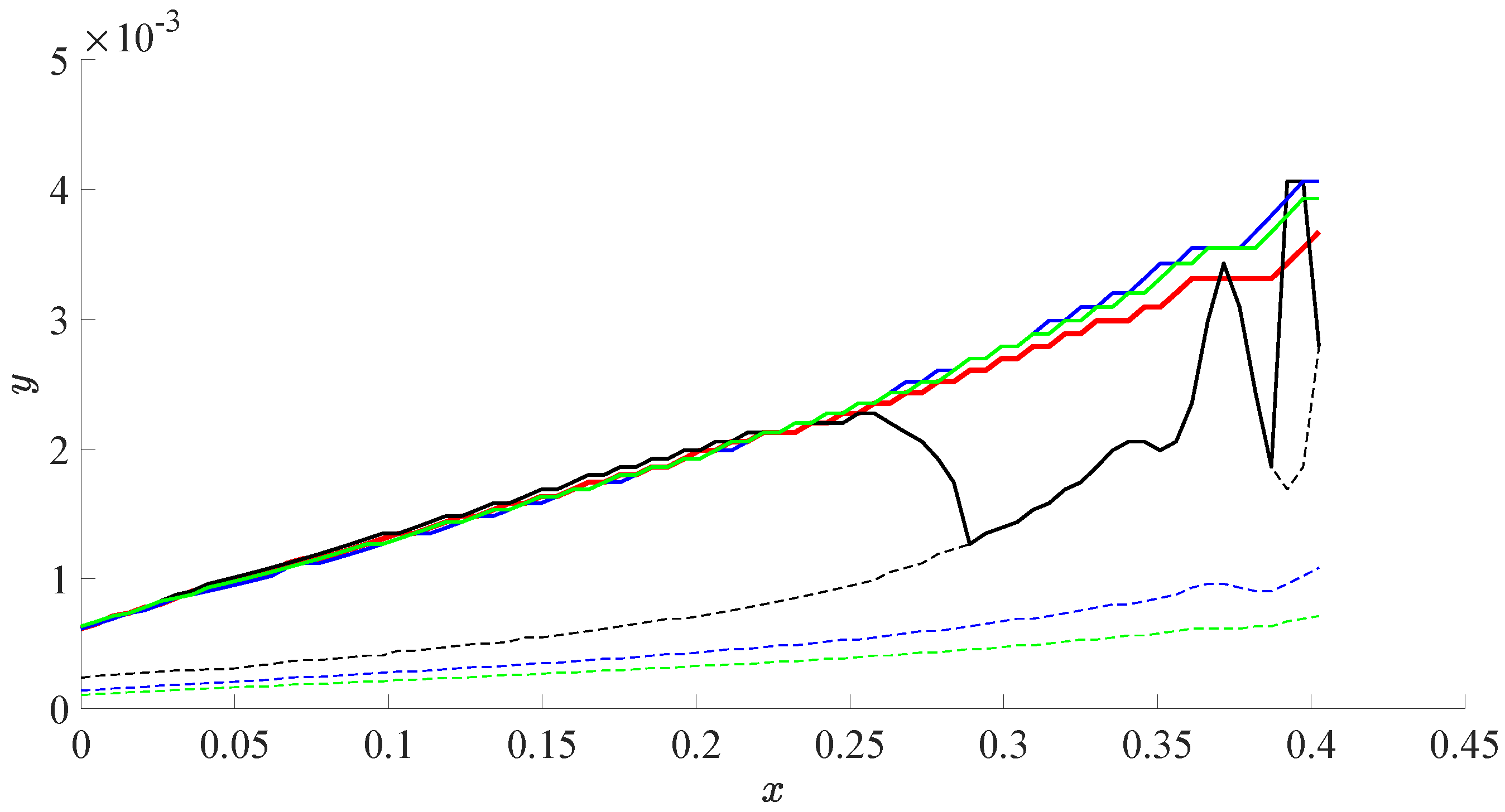
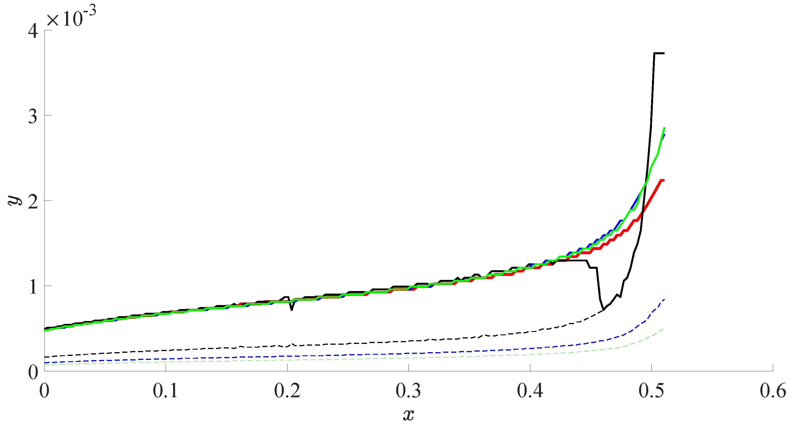
This subsection compares the boundary-layer thickness , obtained by the physically justified method (1), at different values of with , , obtained by the modified probability-based Formulas (5)–(7), respectively. The values of in (1) were chosen so that the stability analysis leads to the adequate results, according to the criteria formulated in Section 4.1. The adjustable constants , , , in the probability-based formulas were chosen by the least squares method to minimize the deviations of , , from along the slice. The distributions of , , , for the slices, which are shown in Figure 1, are presented in Figure 3 and Figure 4. In addition, these figures show the distributions of , , at .
As seen, the function poorly describes the change of boundary-layer thickness along the slice. At first glance, this may be due to the need to compute the wall-normal derivative of the streamwise flux, , near the surface to obtain for as the derivative can be rather inaccurate due to approximation errors. However, this issue appears to be only a minor problem, as can be quite smooth (Figure 4, the black dashed line). The main problem of is similar to that of in (2). It is related to the initial assumption that the function must be non-negative (see the beginning of Section 3.2). If this assumption is not fulfilled, the obtained central moments are able to take negative values. For example, the intersection of the black solid and black dashed lines in Figure 3 and Figure 4 is a consequence of the second wall-normal derivative of changing its sign. Note that the latter is typical for decelerated aerodynamic flows, making the use of inappropriate. In contrast, the functions and with optimal constants and , respectively, are smooth and close to along the slices. The qualitative inferences about the applicability of , , remain valid for the 3D flows under study in various conditions.
Table 1 presents the justified (according to the criteria formulated in Section 4.1) ranges of for various 3D configurations and the corresponding ranges of optimal constants and obtained by the least squares method. It is seen that can be chosen almost the same for each flow-exposed body under study, namely, for the swept wing and for the prolate spheroid. The choice of and approximately complies with all the shown ranges of these constants. Hence, these values can be recommended for all considered configurations. According to the results of our experiments, and are fairly smooth functions of the streamwise coordinate x independently of the considered configuration. This property gives and an advantage because can have significant oscillations along the slice, when the value of is close to or smaller than the accuracy of the main flow computations. Thus, the probability-based estimates of boundary-layer thickness in (6) and in (7) produce quite promising results at least for the considered typical aerodynamic configurations.
5. Conclusions
The probabilistic methods are extended to determine the boundary-layer thickness of the 3D laminar flows of a viscous compressible fluid for the problems of studying the flow instability and predicting the onset of transition to turbulence. The performed numerical experiments show that the application of probabilistic methods is feasible for the considered typical aerodynamic configurations. Values for the parameters of probability-based methods common for all considered configurations are proposed.
Author Contributions
All authors contributed equally to this work. All authors have read and agreed to the published version of the manuscript.
Funding
This research was supported by the Russian Scientific Foundation (grant No. 18-19-00460).
Institutional Review Board Statement
Not applicable.
Informed Consent Statement
Not applicable.
Data Availability Statement
Not applicable.
Conflicts of Interest
The authors declare no conflict of interest.
Abbreviations
The following notations are used throughout the whole manuscript:
| the free stream velocity | |
| the free stream Mach number | |
| the angle of attack | |
| X, Y, Z | the global Cartesian coordinates |
| x, y, z | the local orthogonal coordinates |
| U, V, W | the velocity components in the local coordinates |
| a threshold parameter for determining the boundary-layer thickness based on the stagnation enthalpy | |
| , , | the probability-based boundary-layer thicknesses for compressble 3D flows |
| , , | parameters in the formulas for , , |
| 2D | two-dimensional |
| 3D | three-dimensional |
| LTT | laminar-turbulent transition |
| TS | Tollmien-Schlichting |
| CF | crossflow |
References
- Weyburne, D. A mathematical description of the fluid boundary layer. Appl. Math. Comput. 2006, 175, 1675–1684, Erratum in 2008, 197, 466. [Google Scholar] [CrossRef]
- Weyburne, D. New thickness and shape parameters for the boundary layer velocity profile. Exp. Therm. Fluid Sci. 2014, 54, 22–28. [Google Scholar] [CrossRef]
- Boiko, A.V.; Demyanko, K.V.; Nechepurenko, Y.M. On computing the location of laminar-turbulent transition in compressible boundary layers. Russ. J. Num. Anal. Math. Model. 2017, 32, 1–12. [Google Scholar] [CrossRef] [Green Version]
- Boiko, A.V.; Demyanko, K.V.; Kirilovskiy, S.V.; Nechepurenko, Y.M.; Poplavskaya, T.V. Modeling of transonic transitional three-dimensional flows for aerodynamic applications. AIAA J. 2021. [Google Scholar] [CrossRef]
- Boiko, A.V.; Kirilovskiy, S.V.; Maslov, A.A.; Poplavskaya, T.V. Engineering modeling of the laminar-turbulent transition: Achievements and problems (Review). J. Appl. Mech. Tech. Phys. 2015, 56, 761–776. [Google Scholar] [CrossRef]
- Cebeci, T.; Chen, H.H.; Arnal, D.; Huango, T.T. Three-dimensional linear stability approach to transition on wings and bodies of revolution at incidence. AIAA J. 1991, 29, 2077–2085. [Google Scholar] [CrossRef]
- Krimmelbein, N.; Krumbein, A. Automatic transition prediction for three-dimensional configurations with focus on industrial application. J. Aircraft 2011, 48, 1878–1887. [Google Scholar] [CrossRef]
- Krumbein, A. eN transition prediction for 3D wing configurations using database methods and a local, linear stability code. Aero. Sci. Tech. 2008, 12, 592–598. [Google Scholar] [CrossRef] [Green Version]
- Mack, L.M. Stability of three-dimensional boundary layers on swept wing at transonic speeds. In Symposium Transsonicum III; Zierep, J., Oertel, H., Jr., Eds.; Springer: Berlin/Heidelberg, Germany, 1989; pp. 209–223. [Google Scholar]
- Nayfeh, A.H. Stability of three-dimensional boundary layers. AIAA J. 1980, 18, 406–416. [Google Scholar] [CrossRef] [Green Version]
- Perraud, J.; Arnal, D.; Casalis, G.; Archambaud, J.P.; Donelli, R. Automatic transition predictions using simplified methods. AIAA J. 2009, 47, 2676–2684. [Google Scholar] [CrossRef] [Green Version]
- Gaponenko, V.R.; Ivanov, A.V.; Kachanov, Y.S. Experimental study of a swept-wing boundary-layer stability with respect to unsteady disturbances. Thermophys. Aeromech. 1995, 2, 287–312. [Google Scholar]
- Hirschel, E.H. Basics of Aerothermodynamics; Springer: Berlin/Heidelberg, Germany, 2005; pp. 201–202. [Google Scholar]
- Batchelor, G.K. An Introduction to Fluid Dynamics; Cambridge University Press: Cambridge, UK, 2000. [Google Scholar]
- Schlichting, H.; Gersten, K. Boundary-Layer Theory, 9th ed.; Springer: Berlin/Heidelberg, Germany, 2016. [Google Scholar]
- Ivanov, A.V.; Mischenko, D.A.; Boiko, A.V. Method of the description of the laminar-turbulent transition position on a swept wing in the flow with an enhanced level of free-stream turbulence. J. Appl. Mech. Tech. Phys. 2020, 61, 250–255. [Google Scholar] [CrossRef]
- Kirilovskiy, S.V.; Boiko, A.V.; Demyanko, K.V.; Nechepurenko, Y.M.; Poplavskaya, T.V. Simulation of the laminar-turbulent transition in the boundary layer of the swept wing in the subsonic flow at angles of attack. AIP Conf. Proc. 2020, 2288, 1–6. [Google Scholar]
- Kreplin, H.P.; Vollmers, H.; Meier, H.U. Measurements of the wall shear stress on an inclined prolate spheroid. Z. Flugwiss. Weltraumforsch. 1982, 6, 248–252. [Google Scholar]
- Kreplin, H.P. Three-dimensional boundary layer and flow field data of an inclined prolate spheroid. In AGARD-AR-303: Selection of Experimental Test Cases for the Validation of CFD Codes; AGARD: Neuilly, France, 1994; Volume II, pp. C2.1–C2.12. [Google Scholar]
- Meier, H.U. Experimental investigation of the boundary layer transition and separation on a body of revolution. Z. Flugwiss. Weltraumforsch. 1980, 4, 65–71. [Google Scholar]
- Massey, B.S.; Clayton, B.R. Laminar boundary layers and their separation from curved surfaces. J. Basic Eng. 1965, 87, 483–493. [Google Scholar] [CrossRef]
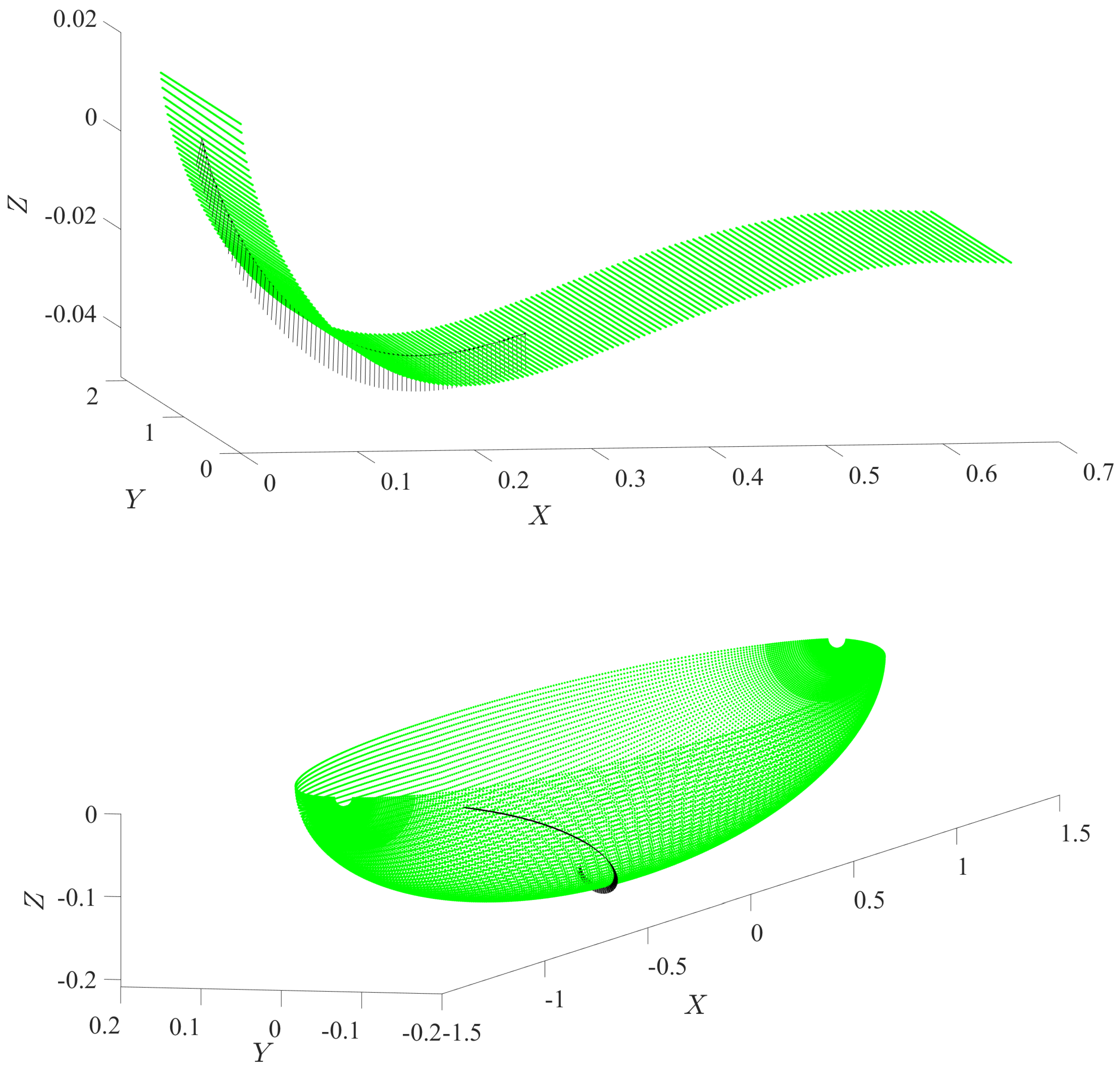
Figure 1.
3D configurations (green) and 2D slices (black) on them in the global Cartesian coordinates X, Y, Z: the lower side wing surface at m/s, (top); half of the prolate spheroid at , rotated counterclockwise by 90 degrees (bottom).
Figure 1.
3D configurations (green) and 2D slices (black) on them in the global Cartesian coordinates X, Y, Z: the lower side wing surface at m/s, (top); half of the prolate spheroid at , rotated counterclockwise by 90 degrees (bottom).

Figure 2.
The U-profiles for each tenth normal of the wing slice (left column), the neutral curves of local temporal stability corresponding to the TS waves (central column; is the local streamwise wave number of disturbances, the red and blue dots denote the beginning and end of the temporal instability region), the N-factor envelope of the growing disturbances (right column): m/s, , (top row), (middle row), (bottom row).

Figure 3.
The function at (red), and the functions (black), (blue), (green) at optimal values of adjustable constants , , (solid line) and at (dashed line) for the slice at the wing in Figure 1.
Figure 3.
The function at (red), and the functions (black), (blue), (green) at optimal values of adjustable constants , , (solid line) and at (dashed line) for the slice at the wing in Figure 1.

Figure 4.
The function at (red), and the functions (black), (blue), (green) at optimal values of adjustable constants , , (solid line) and at (dashed line) for the slice at the prolate spheroid in Figure 1.
Figure 4.
The function at (red), and the functions (black), (blue), (green) at optimal values of adjustable constants , , (solid line) and at (dashed line) for the slice at the prolate spheroid in Figure 1.


Table 1.
Adequate ranges of for the swept wing (at different values of and for different 2D slices) and for the prolate spheroid (at different values of and for different 2D slices) and corresponding ranges of optimal constants , . The considered slices are located on the lower or upper sides of the wing, and on the lower, middle and upper parts of the prolate spheroid.
| Parameters (the Slice Position) | p | |||
|---|---|---|---|---|
| Swept wing | , (lower) | 3.73–4.98 | 4.83–6.30 | |
| , (upper) | 3.80–5.06 | 4.84–6.30 | ||
| , (lower) | 3.62–6.14 | 4.70–7.67 | ||
| , (lower) | 3.83–9.74 | 4.94–11.9 | ||
| , (upper) | 3.79–8.82 | 4.86–10.7 | ||
| , (upper) | 3.78–7.15 | 4.80–8.75 | ||
| Prolate spheroid | , (lower) | 3.73–6.96 | 3.79–6.59 | |
| , (middle) | 3.73–6.61 | 4.07–6.77 | ||
| , (upper) | 4.01–5.23 | 5.10–6.51 | ||
| , (middle) | 5.09–6.27 | 6.44–7.82 | ||
| , (lower) | 3.04–6.53 | 4.02–8.11 | ||
| , (middle) | 3.00–6.43 | 3.99–8.03 | ||
| , (upper) | 4.06–4.92 | 5.15–6.30 | ||
| , (middle) | 4.09–5.86 | 5.32–7.41 |
Publisher’s Note: MDPI stays neutral with regard to jurisdictional claims in published maps and institutional affiliations. |
© 2021 by the authors. Licensee MDPI, Basel, Switzerland. This article is an open access article distributed under the terms and conditions of the Creative Commons Attribution (CC BY) license (https://creativecommons.org/licenses/by/4.0/).
Share and Cite
MDPI and ACS Style
Boiko, A.V.; Demyanko, K.V.; Nechepurenko, Y.M.; Zasko, G.V. On the Use of Probability-Based Methods for Estimating the Aerodynamic Boundary-Layer Thickness. Fluids 2021, 6, 267. https://0-doi-org.brum.beds.ac.uk/10.3390/fluids6080267
AMA Style
Boiko AV, Demyanko KV, Nechepurenko YM, Zasko GV. On the Use of Probability-Based Methods for Estimating the Aerodynamic Boundary-Layer Thickness. Fluids. 2021; 6(8):267. https://0-doi-org.brum.beds.ac.uk/10.3390/fluids6080267
Chicago/Turabian StyleBoiko, Andrey V., Kirill V. Demyanko, Yuri M. Nechepurenko, and Grigory V. Zasko. 2021. "On the Use of Probability-Based Methods for Estimating the Aerodynamic Boundary-Layer Thickness" Fluids 6, no. 8: 267. https://0-doi-org.brum.beds.ac.uk/10.3390/fluids6080267