Turbulent Non-Stationary Reactive Flow in a Cement Kiln

Abstract

The reduction of emissions from large industrial furnaces critically relies on insights gained from numerical models of turbulent non-premixed combustion. In the article Mitigating Thermal NOx by Changing the Secondary Air Injection Channel: A Case Study in the Cement Industry, the authors present the use of the open-source OpenFoam software environment for the modeling of the combustion of Dutch natural gas in a cement kiln operated by our industrial partner. In this paper, various model enhancements are discussed. The steady-state Reynolds-Averaged Navier-Stokes formulation is replaced by an unsteady variant to capture the time variation of the averaged quantities. The infinitely fast eddy-dissipation combustion model is exchanged with the eddy-dissipation concept for combustion to account for the finite-rate chemistry of the combustion reactions. The injection of the gaseous fuel through the nozzles occurs at such a high velocity that a comprehensive flow formulation is required. Unlike in Mitigating Thermal NOx by Changing the Secondary Air Injection Channel: A Case Study in the Cement Industry, wave transmissive boundary conditions are imposed to avoid spurious reflections from the outlet patch. These model enhancements result in stable convergence of the time-stepping iteration. This in turn increases the resolution of the flow, combustion, and radiative heat transfer in the kiln. This resolution allows for a more accurate assessment of the thermal NO-formation in the kiln. Results of a test case of academic interest are presented. In this test case, the combustion air is injected at a low-mass flow rate. Numerical results show that the flow in the vicinity of the hot end of the kiln is unsteady. A vortex intermittently transports a fraction of methane into the air stream and a spurious reaction front is formed. This front causes a transient peak in the top wall temperature. The simulated combustion process is fuel-rich. All the oxygen is depleted after traveling a few diameters into the kiln. The thermal nitric oxide is formed near the burner and diluted before reaching the outlet. At the outlet, the simulated thermal NO concentration is equal to 1 ppm. The model is shown to be sufficiently mature to capture a more realistic mass inflow rate in the next stage of the work.

1. Introduction

Rotary kilns are long cylindrical furnaces used for the production of cement and other material processing applications [1]. These furnaces have been studied extensively both numerically [2,3,4] and experimentally [5,6].

We studied the kiln previously described in [7]. It is used by our industrial partner for the production of specialty cement used in niche applications. The combustion is fed by the injection of Dutch natural gas through a multi-nozzle burner mounted at the end of the centrally mounted burner pipe. The burner consists of an inner ring of outward inclined nozzles and an outer ring of axial nozzles. Air is provided via two channels. A minor quantity of primary air flows through a burner slot encircling the outer nozzles. The bulk of secondary air is injected through a rectangular slot above the attachment of the burner pipe. The aerodynamics inside the kiln that cause the mixing of fuel and oxidizer can be decomposed into two components. The first is the bluff body flow caused by the inflow of secondary air. The second is the jet formed by the merging of the individual jets originating from the burner nozzles. The combination of the flow components in co-flow causes the fuel and oxidizer to mix. The heat released by the ensuing chemical reactions is transferred to the material bed mainly by radiative transfer. The kiln operates at high temperatures. The process is thus prone to the formation of thermal nitric oxides. The objective of this paper is to model the process of thermal NO formation in the kiln. Insights gained will be used to formulate design improvements to mitigate thermal NO formation in a second stage.

The short-term goal of this paper is to arrive at a simulation model for the combustion in the kiln implemented in open-source software that converges in a stable and reliable manner. The reliance on open-source software opens the possibilities for wider use of this technology by our industrial partner. Reliable convergence allows the accurate prediction of the pollutant emissions from the combustion that is urgently required. Longer term goals of this work include gaining a better understanding of the pollutant emissions in existing operational units and aiding in the design of next-generation furnaces.

In this paper, we restrict ourselves to the modeling of the reactive flow of the gasses and heat transfer in the freeboard of the kiln. The conjugate heat transfer to the insulating lining is left out of consideration. We instead impose thermal insulating boundary conditions on the interface between freeboard gasses and the lining. We stay away from realistic operating conditions. We consider the hypothetical case of a low-mass flow rate of combustion air in which the mixture is fuel-rich. We furthermore do not take into account the presence of a material bed and model the empty kiln. In this way, we stay away from confidential information from our industrial partner. Like in [7], we employ the open-source software environment OpenFoam [8]. We refrain from comparison with experimental data. This paper should be viewed as a methodological study.

The single and most important scientific contribution of this paper is the development of a model for combustion in the kiln that converges stably and reliably. This convergence is of the utmost importance to assess the thermal nitric oxide formation in a meaningful manner. To arrive at a stable convergence, the model previously published in [7] is adapted in various ways. In [7], we employed a steady-state Reynolds-Averaged Navier-Stokes (RANS) model to describe the flow of the mixture of gasses in the freeboard of the kiln. This steady-state formulation fails to converge in the absence of a physical steady-state. In a first model improvement, the steady-state model was replaced with an unsteady formulation in this paper. The latter tracks the time-variation of the Favre averaged quantities as described in e.g., [9] and references cited therein. The time-step $△t$ in the transient simulation using the PIMPLE algorithm is fixed to $△t=1\times {10}^{-5}$. In post-processing, a spectral analysis in the time domain reveals the characteristic frequencies of the various fields at various probe locations. The speed of the gaseous fuel leaving the burner is so high that Mach numbers as high as 0.6 are reached. The flow can thus no longer be treated as incompressible. We thus adopt a compressible OpenFoam solver with thermodynamics based on compressibility with solver settings that include the divergence term in the pressure equation. In a second model improvement, we employ in this paper a wave-transmissive boundary condition for the pressure at the outlet to avoid pressure waves traveling from the outlet into the computational domain. In [7], we employed the eddy–dissipation model for combustion in OpenFoam. The formulation in OpenFoam, however, deviates from the standard implementation, making the comparison with any benchmark results problematic. In a third model improvement, we replaced the eddy–dissipation model for infinitely fast turbulent combustion in [7] with the eddy–dissipation concept for combustion that takes finite rate chemistry into account. The EDC combustion model is based on the energy transfer from large-scale to smaller-scale eddies in the turbulent flow [10,11]. Other modifications to [7] that contribute to arriving at a stable converging model include changes in the geometrical representation of the inlet section of the inclined nozzles of the burner, the mesh, and the inlet conditions.

The introduction of the transient model reveals the pulsating nature of the flow near the burner outlets. Further downstream, the flow relaxes to a state that changes slower in time. We analyze the temporal frequency of the pressure, the velocity components, and the temperature at various locations on the center axis of the kiln. The fuel and oxidizer mix at the hot end of the kiln. At t he hot end, the physical fields are shown to vary in time at frequencies higher than the acoustic resonant frequency of the cylinder equal to $6.65\mathrm{Hz}$. The kiln acts as a low-pass filter in time, and the frequency content of the fields reduces while moving toward the cold end. At the outlet, only a few low frequencies remain. The outlet pressure varies at a single dominant frequency equal to the resonant frequency. The dominant frequency of the axial and transversal velocity components at the outlet is significantly lower than $6.65\mathrm{Hz}$. The mode of the outlet axial velocity at $6.65\mathrm{Hz}$ is three times smaller than its lower frequency dominant mode. The outlet transversal velocity components have a negligibly small $6.65\mathrm{Hz}$ mode. The outlet temperature varies in time at an even slower rate. The low-mass flow rate of combustion air causes a fraction of methane to recirculate into the air stream. A spurious reaction front and transitory peak in the wall temperature form.

The remainder of this paper is structured in five sections. In Section 2, the geometry definition, the mesh generation, and the setting of the boundary conditions are discussed. In Section 3 and Section 4, the combustion model employed and its implementation in OpenFoam are introduced, respectively. In Section 5, the numerical results are presented. Finally, in Section 6, some conclusions from the work are drawn.

2. Material

In this section, we describe the geometry of the kiln and the mesh used for the combustion simulation of the freeboard gasses.

2.1. Geometry Definition

We represent the kiln on a one-to-one scale. We employ the same geometry as before in [7] with the insulating lining removed. The geometry consists of a long cylinder. A burner pipe is co-axially mounted at the hot end of the cylinder as shown in Figure 1. At the end of the burner pipe, the burner is mounted. On top of the mount of the burner pipe, the rectangular secondary air inlet is located. The cold end of the cylinder is considered to be open.

The burner consists of two sets of eight nozzles placed equidistantly along concentric circles. The nozzles on the inner and outer circle are oriented outward and axially, respectively. A cooling slot encircles the nozzles. Given its importance for the mixing of the fuel, we accurately represent the burner in our geometry. Unlike in [7], we represent the inlet sections of the inclined fuel nozzles by disks perpendicular to the axis of the inclined nozzles. This aids the convergence of the numerical simulation of the fluid injected through these nozzles.

The small diameter of the fuel nozzles immersed in the long kiln renders the mesh generation especially challenging. The mass flow rate through the nozzles is sufficiently large for the assumptions of incompressible flow to no longer apply. Resorting to transonic flow computation thus becomes mandatory.

2.2. Mesh Generation

The mesh for the combustion simulations consisting of about $1.1$ million cells was generated using the cfMesh package [12]. Local refinement near the outlet of the fuel nozzles and near the walls was applied. The former and latter are intended to resolve the high speed of the fuel injection heat transfer through the walls, respectively. The mesh in the vicinity of the hot end of the kiln is shown in Figure 1. Various details on the mesh employed can be found in Appendix A.

2.3. Imposed Boundary Conditions

We apply a nominal-mass inflow rate at room temperature for the inflow of gaseous fuel through the burner. We apply a significantly smaller than nominal mass inflow for the preheated air through the secondary air inlet. These inflow conditions are illustrated in Figure 2. With the air inflow condition, the volumetric air-to-gas ratio is equal to 4.5, and the mixture is fuel-rich. The thermal NO mass fraction at the outlet will be negligibly small. The case becomes of academic interest and a reference for future computations. It also allows us to conceal sensitive information of our industrial partner. At the outlet, we prescribe wave transmissive condition for the pressure. At the walls, we employ standard wall functions, a constant thermal absorption coefficient equal to $\kappa =0.7{\mathrm{m}}^{-1}$ and a wall emissivity value equal to ${ϵ}_w=0.7[-]$.

3. Method

In this section, we present the model for the non-premixed turbulent combustion in the kiln that we will solve using OpenFoam. This model consists of three submodels. The first is a description of the non-stationary and non-isothermal turbulent flow of the mixture of pre-heated air and gaseous fuel. The second is a description of the transport by diffusion and by convection of the individual chemical species. The transport equations include sink and source terms for the depletion of the oxidizer and the fuel and the creation of combustion products, respectively. The third is a description of the radiative heat transport in the participating media. The thermal nitric oxide mass fraction is computed in the post-processing stage. For details on the modeling of turbulent flow, turbulent combustion and pollutant formation, we refer to references such as, e.g., [13,14,15,16,17]. More information on the modeling of radiative heat transfer can be found in, e.g., [18].

We denote by ${\mu }_0$ and ${\lambda }_0$ the molecular viscosity and the molecular thermal conductivity of the gas mixture. Modeling of combustion requires tracking the individual chemical species. We denote their mass fraction as $Y_s$ for $s\in \{1,\dots ,Ns\}$. The heat capacity at constant pressure of the gas mixture $C_p(T,Y_s)$ is computed as the weighted average of the heat capacity of the individual species. The thermal absorption coefficient $\kappa$ is assumed to be a constant in this paper.

The Mach number of the flow of the gas mixture reaches values as large as 0.6. Compressible formulation is thus required. We employ an unsteady Reynolds-Averaged model with Favre averaging closed by the standard k-$\epsilon$ two-equation turbulence model for the turbulent kinetic energy k and the eddy dissipation rate $\epsilon$, respectively. The choice for the k-$ϵ$ turbulence model is motivated by the wish to compare with the results in previous work and to rely on well-established models in OpenFoam. Let $\overline{\rho }$ denote the Reynolds-Averaged mass density. Using k and $\epsilon$, the turbulent mixing time scale ${\tau }_t$, the turbulent eddy viscosity ${\mu }_t$ and the turbulent kinematic viscosity ${\nu }_t$ are defined as

$${\tau }_t=\frac{k}{\epsilon },{\mu }_t=\overline{\rho }{C}_{\mu }\frac{k^2}{\epsilon },\mathrm{and}{\nu }_t=\frac{{\mu }_t}{\overline{\rho }},$$

(1)

respectively. $C_{\mu }$ is a model constant equal to $0.09$.

We assume that the combustion occurs in a regime in which diffusion flames with thin reaction fronts are formed. In this regime, the turbulent mixing time scale dominates the chemical time scale. The Damkohler number is thus much larger than one. To model the combustion, we employ the eddy dissipation concept [10,11].

We simplify Dutch natural gas to methane as its main component. We adapt the single step irreversible global reaction mechanism

$$\mathrm{C}{\mathrm{H}}_4+2({\mathrm{O}}_2+3.76{\mathrm{N}}_2)\to \mathrm{C}{\mathrm{O}}_2+2{\mathrm{H}}_2\mathrm{O}+7.52{\mathrm{N}}_2,$$

(2)

which has an enthalpy of combustion equal to $△h_{fuel}=-802,310\mathrm{kJ}/\mathrm{kmol}$ of CH${}_4$. We thus need to track the mass fraction of $Ns=4$ chemical species. The presence of the inert N${}_2$ facilitates numerically enforcing that the mass fractions sum up to one.

Various models that capture the radiative heat transfer to various degrees of accuracy are available in the literature. The P1-model requires solving a non-linear diffusion equation for a single scalar field at each update of the radiative field. Therefore, it offers a good compromise between the model accuracy and the computational cost and is therefore adopted in this paper. We neglect any effect of scattering. The P1-model assumes the medium to be isotropic in space for radiative transfer. This approximation is valid in the case that the medium has a large optical thickness.

In the remainder of this section, we describe the governing equations and boundary conditions in more detail.

3.1. Flow of Mixture of Gasses in the Flue

We solve the turbulent compressible transient Navier–Stokes system that expresses the conservation of mass, momentum, and energy of the non-isothermal flowing gas mixture in a transonic regime. The density of the mixture varies in space due to the heat released by combustion. Density, pressure and temperature are linked by the ideal gas equation of state. Turbulent fluctuations are taken into account by density-weighted Reynolds averaging. The standard k-epsilon turbulence model ensures closure.

We employ Favre or density-weighted averaging [16]. This averaging is performed as follows

$$\xi =\tilde{\xi }+{\xi }^{″}\mathrm{where}\tilde{\xi }=\frac{\overline{\rho \xi }}{\overline{\rho }}.$$

3.1.1. Conservation of Mass of the Mixture

After Favre averaging, the conversation of mass of the gas mixture can be expressed as

$$\frac{\partial \overline{\rho }}{\partial t}+\frac{\partial \overline{\rho }{\tilde{u}}_i}{\partial x_i}=0,$$

(3)

where $\overline{\rho }$ is the Reynolds-Averaged density of the mixture, and ${\tilde{u}}_i$ is the Favre average of the three velocity components, respectively.

3.1.2. Conservation of Momentum of the Mixture

The viscous part of the deformation matrix $s_{ij}^{\prime }$ is given by

$$s_{ij}^{\prime }=\frac{\partial {\tilde{u}}_i}{\partial x_j}+\frac{\partial {\tilde{u}}_j}{\partial x_i}.$$

(4)

The turbulent kinetic energy k and its dissipation rate $\epsilon$ are defined by

$$k=\frac{1}{2}\sum _{j=1}^3\widetilde{u_j^{″}{u}_j^{″}}\mathrm{and}\epsilon =2\frac{{\mu }_0}{\overline{\rho }}\sum _{i,j=1}^3\widetilde{s_{ij}^{\prime }{s}_{ij}^{\prime }}.$$

(5)

Using the Boussinesq hypothesis, the conservation of momentum of the gas mixture can be expressed as

$$\frac{\partial }{\partial t}\left(\overline{\rho }{\tilde{u}}_i\right)+\frac{\partial }{\partial x_j}\left(\overline{\rho }{\tilde{u}}_j{\tilde{u}}_i\right)=\frac{\partial }{\partial x_j}\left[({\mu }_0+{\mu }_t)\left(\frac{\partial {\tilde{u}}_i}{\partial x_j}+\frac{\partial {\tilde{u}}_j}{\partial x_i}\right)\right]-\frac{2}{3}\frac{\partial }{\partial x_i}\left[{\mu }_t\frac{\partial {\tilde{u}}_m}{\partial x_m}\right]-\frac{2}{3}\frac{\partial }{\partial x_i}\left[\overline{\rho }k\right]-\frac{\partial \tilde{p}}{\partial x_i},$$

(6)

for $j\in \{1,2,3\}$, where $\tilde{p}$ and k denote the Favre averaged pressure and turbulent kinetic energy, respectively. The transport equations for the turbulent kinetic energy k and its dissipation rate $\epsilon$ are given by the standard k-$\epsilon$ [14] model as

$$\frac{\partial }{\partial t}\left(\overline{\rho }k\right)+\frac{\partial }{\partial x_j}\left(\overline{\rho }{\tilde{u}}_{j}k\right)=\frac{\partial }{\partial x_j}\left[\frac{{\mu }_t}{{\sigma }_k}\frac{\partial k}{\partial x_j}\right]+2{\mu }_t{\tilde{s}}_{ij}{\tilde{s}}_{ij}-\overline{\rho }\epsilon$$

(7)

$$\frac{\partial }{\partial t}\left(\overline{\rho }\epsilon \right)+\frac{\partial }{\partial x_j}\left(\overline{\rho }{\tilde{u}}_j\epsilon \right)=\frac{\partial }{\partial x_j}\left[\frac{{\mu }_t}{{\sigma }_{\epsilon }}\frac{\partial \epsilon }{\partial x_j}\right]+C_{1\epsilon }\frac{\epsilon }{k}2{\mu }_t{\tilde{s}}_{ij}{\tilde{s}}_{ij}-C_{2\epsilon }\overline{\rho }\frac{{\epsilon }^2}{k},$$

(8)

where ${\sigma }_k$ and ${\sigma }_{\epsilon }$ are the turbulent Prandtl numbers for k and $\epsilon$, respectively. $C_{1\epsilon }=1.44$ and $C_{2\epsilon }=1.92$ are model constants. Standard wall functions are used. The flow sub-model is solved for the average pressure, the average velocity components and the turbulent quantities k and $\epsilon$. Large values of ${\nu }_t$ indicate strong mixing of the fuel and the oxidizer.

3.1.3. Conservation of Energy of the Mixture

We will express the conservation of energy of the mixture using the sensible enthalpy $h_s$ with the Favre average denoted by ${\tilde{h}}_s$. We neglect all body forces except for the heat generated by combustion and the heat transport by radiation. The contribution of diffusive transport by the individual species and viscous heating is neglected. We neglect the Soret and Dufour effect and assume that the Lewis number is equal to one. With these assumptions, the transport equation for sensible enthalpy can then be written as

$$\frac{\partial }{\partial t}(\overline{\rho }{\tilde{h}}_s)+\frac{\partial }{\partial x_i}(\overline{\rho }{\tilde{u}}_i{\tilde{h}}_s)=\frac{\partial }{\partial x_i}\left[({\lambda }_0+\frac{{\mu }_t}{{\sigma }_T})\frac{\partial \tilde{T}}{\partial x_i}\right]+\frac{\partial \tilde{p}}{\partial t}+{\tilde{u}}_i\frac{\partial \tilde{p}}{\partial x_i}+{\tilde{\dot{Q}}}_{chem}+{\tilde{\dot{Q}}}_{rad},$$

(9)

where ${\sigma }_T$ is the Prandtl number for the transport of temperature. The source terms ${\tilde{\dot{Q}}}_{chem}$ and ${\tilde{\dot{Q}}}_{rad}$ represent the heat release due to combustion and the heat transport due to radiation, respectively. In case the EDC model for combustion is used, ${\tilde{\dot{Q}}}_{chem}$ is given by

$${\tilde{\dot{Q}}}_{chem}=△h_{fuel}{\dot{\omega }}_{fuel},$$

(10)

where $△h_{fuel}$ and ${\dot{\omega }}_{fuel}$ are the heat of combustion of the fuel and the chemical source term for the fuel. The value for $△h_{fuel}$ is given after Equation (2). The expression for ${\dot{\omega }}_{fuel}$ is given by the EDC combustion model. In case the P1 model for radiative heat transfer is used, ${\tilde{\dot{Q}}}_{rad}$ is given by

$${\tilde{\dot{Q}}}_{rad}=-\frac{\partial q_{rad,j}}{\partial x_j}=\tilde{\kappa }\tilde{G}-4\pi \sigma {\left(\tilde{T}\right)}^4$$

(11)

where $\tilde{\kappa }=\kappa =0.7{\mathrm{m}}^{-1}$; $\sigma =5.67e^{-8}[W/m^2{K}^4]$ is the Stefan–Boltzmann constant. Here we assume that the Favre average of the product of $\kappa$ and G is given by the product of the Favre averages of $\kappa$ and G. Similarly, we assume that the Favre average of the fourth power of T is given by the fourth power of the Favre average of T. No turbulence–radiation interaction is thus taken into account.

3.1.4. Conservation of the Chemical Species

The concentration of the individual chemical species $Y_s$ with the Favre average ${\tilde{Y}}_s$ for $s\in \{1,\dots ,4\}$ is governed by a set of convection–diffusion–reaction with source term ${\tilde{\dot{\omega }}}_s$ given by the eddy dissipation combustion model. We assume that all species have the same molecular mass diffusivity denoted by $D_0$. The Favre-averaged equations for conservation of $Y_s$ can be written as

$$\begin{array}{c}\hfill \frac{\partial }{\partial t}\left(\overline{\rho }{\tilde{Y}}_s\right)+\frac{\partial }{\partial x_i}\left(\overline{\rho }{\tilde{u}}_i{\tilde{Y}}_s\right)=\frac{\partial }{\partial x_i}\left[\overline{\rho }(D_0+\frac{{\mu }_t}{S{c}_t})\frac{\partial {\tilde{Y}}_s}{\partial x_i}\right]+{\tilde{\dot{\omega }}}_s,\end{array}$$

(12)

where $S{c}_t$ is the turbulent Schmidt number for the transport of species. Suitable inlet conditions need to be imposed for $Y_{CH4}$ and $Y_{O2}$ on the inlet patch for the burner and air inlet, respectively. Required values for $\overline{\rho }$, ${\tilde{u}}_i$ and ${\mu }_t$ follow from a previously discussed flow model. Computed values for ${\tilde{Y}}_s$ allow us to recompute $\overline{\rho }$ and the combustion heat release term ${\tilde{\dot{Q}}}_{chem}$.

3.1.5. Computation of the Radiative Heat Flux

In the P1-model for radiative heat transfer, the total radiative intensity G with the Favre average $\tilde{G}$ is governed by the following diffusion equation

$$\frac{\partial }{\partial x_j}\left(\frac{1}{3\tilde{\kappa }}\frac{\partial \tilde{G}}{\partial x_j}\right)=\tilde{\kappa }\tilde{G}-4\tilde{\kappa }\sigma {\left(\tilde{T}\right)}^4.$$

(13)

The boundary condition requires introducing the wall emissivity denoted by ${ϵ}_w$. This emissivity is set to 0 on the symmetry patch, to 1 on the inlet and outlet patches and equal to $0.7$ on all other patches. The Marshak boundary condition for $\tilde{G}$ can then be expressed as

$$\frac{2}{3\tilde{\kappa }}\frac{\partial \tilde{G}}{\partial x_j}{n}_j=\frac{{ϵ}_w}{2-{ϵ}_w}[\tilde{G}-4\sigma {\left(\tilde{T}\right)}^4],$$

(14)

where the vector with component $n_j$ is the unit normal vector on the boundary patch. The solution for $\tilde{G}$ allows us to update the radiative source term ${\tilde{\dot{Q}}}_{rad}$.

3.2. Zeldovich Thermal nitric oxide Post-Processing

The thermal nitric oxide concentration is computed in the post-processing stage using a three-step Zeldovich mechanism described in, e.g., [14]. For the O and OH concentration required as input, equilibrium chemistry is assumed. The implementation in the NOxFoam solver is described in the master thesis [19].

4. Implementation in OpenFOAM

The set of conservation equations introduced above is discretized in space using a cell-centered finite volume method and a finite difference method in time. The resulting set of ordinary differential equations is integrated in time using the PIMPLE algorithm implemented in the reactingFoam solver. The equations in the flue domain are solved segregated by an extension of the PIMPLE algorithm for the velocity–pressure coupling that takes the variability of density into account. At each pressure–velocity–energy iteration, the transport equations for the turbulent kinetic energy k, the turbulent dissipation rate $\epsilon$, the chemical species ${\tilde{Y}}_s$ and the total incident radiation $\tilde{G}$ are solved to be able to update the turbulent viscosity ${\mu }_t$ and the source terms ${\tilde{\dot{Q}}}_{chem}$ and ${\tilde{\dot{Q}}}_{rad}$ in the energy equation. The linear systems that arise from the discretization of the separate fields are solved by a suitably preconditioned Krylov subspace method.

As in [7], we perform numerical simulations using OpenFoam-v2012. Unlike in [7], we implemented the following three changes.

We replaced the steady-state Reynolds-Averaged Navier–Stokes model with an unsteady (URANS) variant. This transient model captures the pulsating nature of the jets leaving the burner nozzles. For more details on URANS, we refer to, e.g., [9] and references cited therein. On the outlet, we apply a wave-transmissive boundary condition for the pressure with an appropriate setting of the parameter $L_{inf}$ [20]. As the combustion model, we use the Eddy Dissipation Concept [10,11] with default parameter settings.

5. Numerical Results

In this section, we report the numerical results obtained from running the model until $t=60\mathrm{s}$. We report on the computed mass species fraction, the computed wall temperature, and the time frequency of the flow field.

5.1. Computed Species Mass Fraction

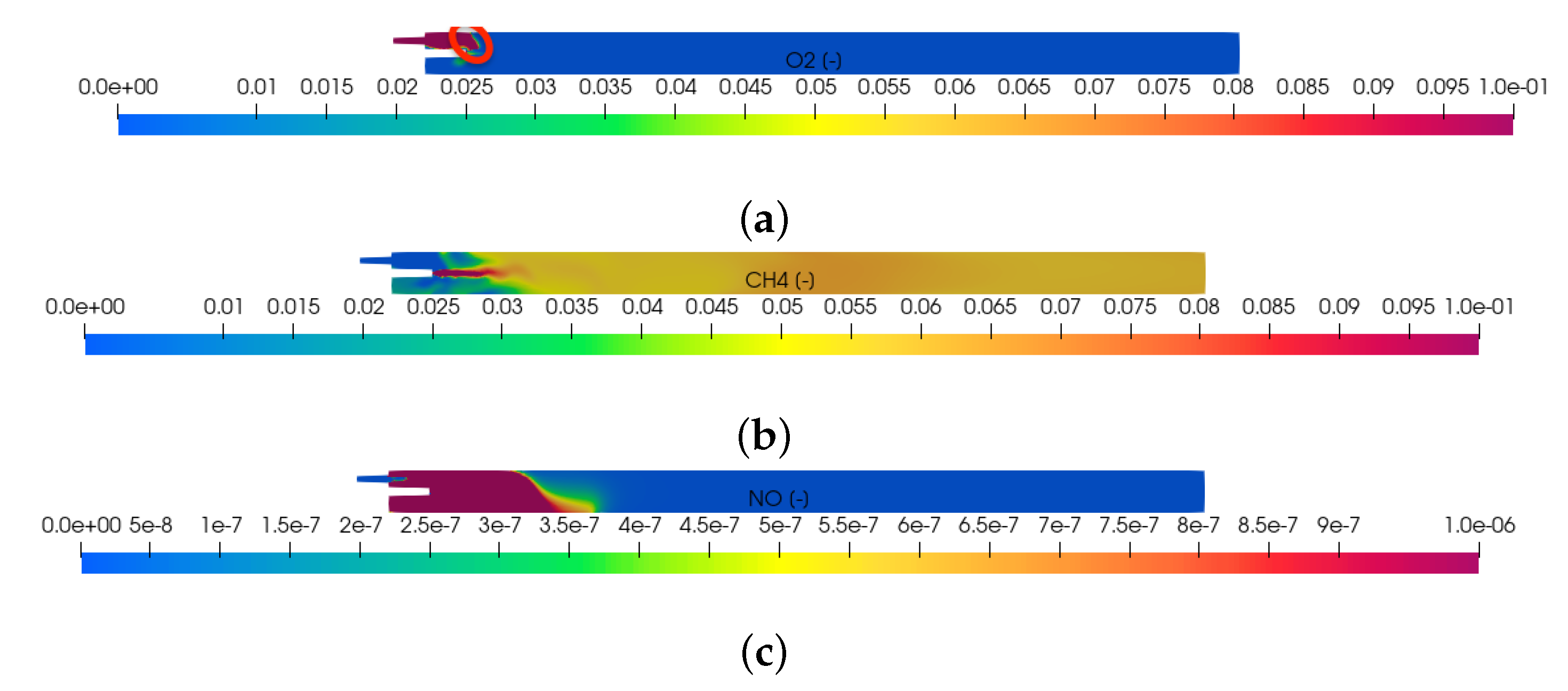
The computed mass fraction of oxygen, methane and thermal nitric oxide on the middle axial plane ($xz$-plane at $y=0$) at $t=60\mathrm{s}$ are shown in Figure 2. The case considered is fuel-rich. Not enough air is injected into the furnace to combust all the available methane. The oxygen mass fraction becomes zero downstream of a thin reaction front indicated in red in the top figure. Downstream from the reaction zone, the mass fraction of methane is reduced by dilution in its surroundings. Five percent of the injected methane reached the outlet without being combusted. The thermal NO formed is seen to be the largest at the hot end of the kiln. It is diluted when transported to the cold end. At the outlet, the mass fraction of thermal NO is equal to 1 ppm. As the air-to-gas ratio is increased from the current fuel-rich value of 4.5 to its stoichiometric value, we expect the air to penetrate further into the furnace, a broader reaction front, and more thermal NO to form.

5.2. Computed Wall Temperature

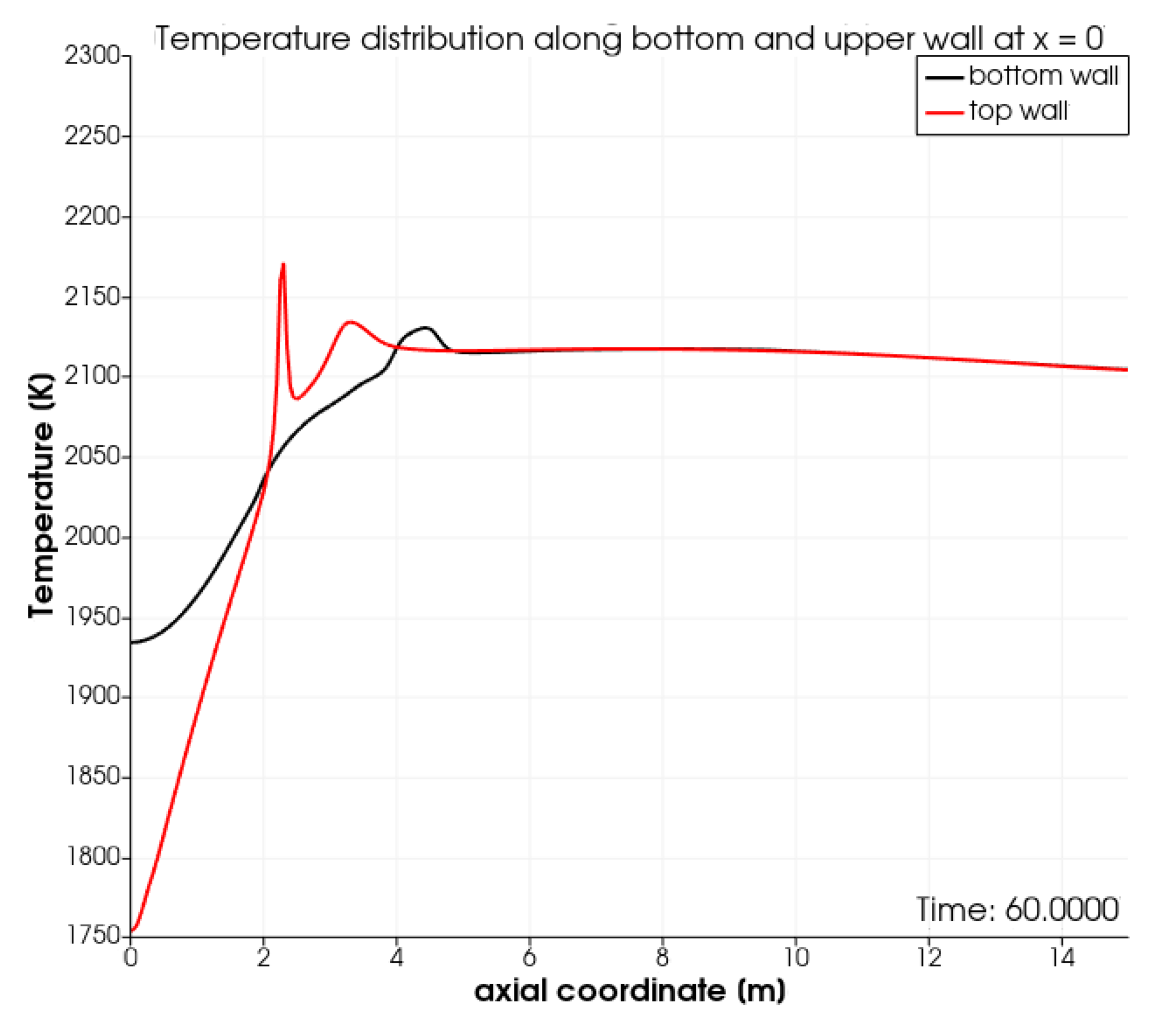
The computed wall temperature on the top and bottom wall along the first 15 meters of the kiln is shown in Figure 3. Initially, the top wall is cooler than the bottom wall. This is due to the cooling effect of the combustion air injected above the burner pipe and the recirculation of the hot combustion gasses underneath the fuel pipe. The cooling effect of the combustion air was also discussed in [21]. Subsequently, the top wall becomes hotter than the bottom wall due to the combustion in the thin reaction zone highlighted in Figure 2. At higher air-to-gas ratios, we expect the peak in temperature to become broader. In the latter scenario, the results generated using OpenFoam will better match the results from the commercial CFD package reported in [21].

Both Figure 2 and Figure 3 show a snapshot at $t=60\mathrm{s}$. The flow field, the species mass fractions and the temperature near the hot end of the kiln, however, fluctuate. This will be elaborated further in this subsection.

5.3. Frequency of Time Traces

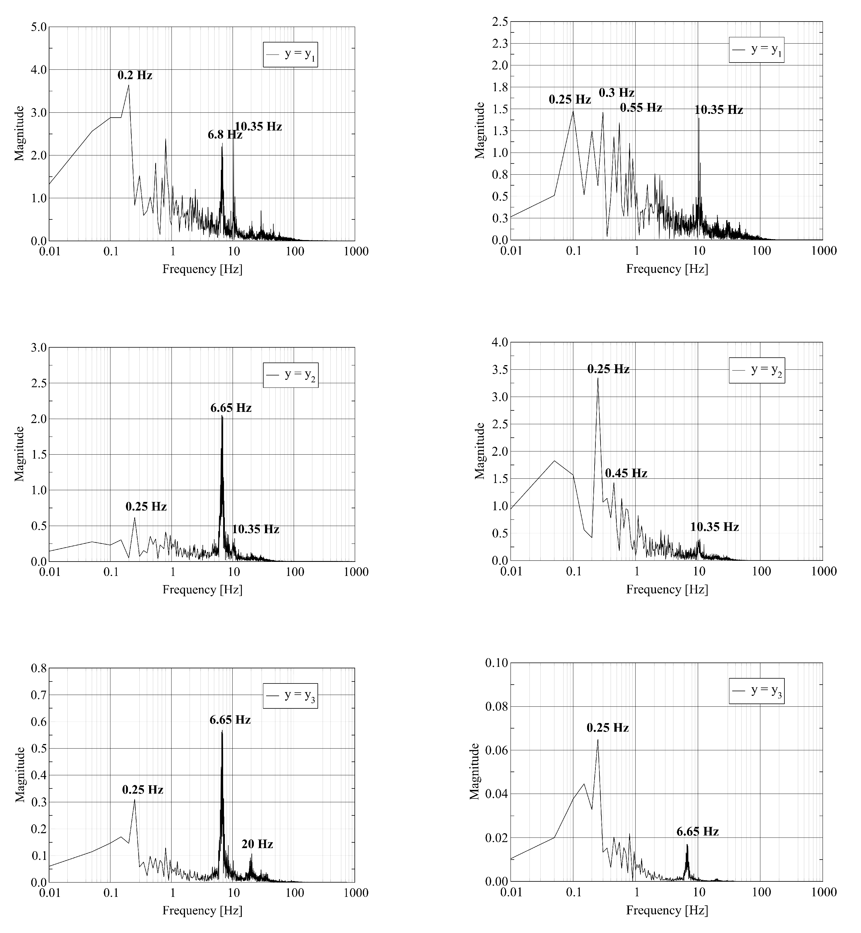
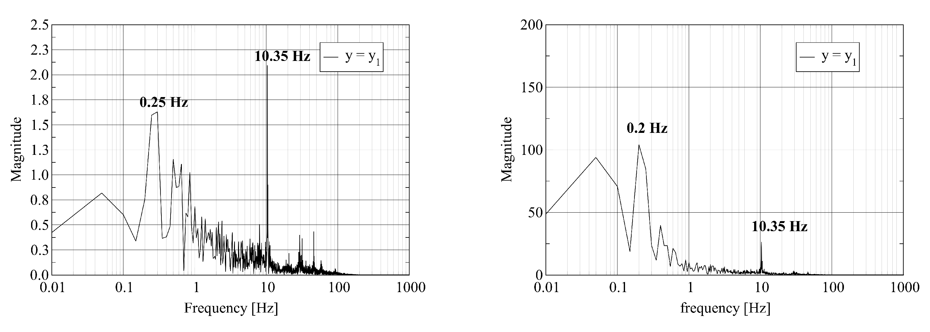
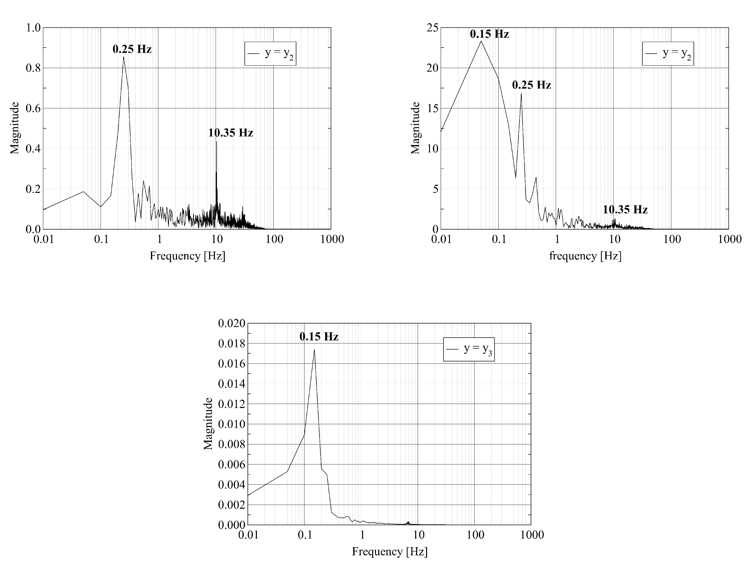
The visualization of the computed axial velocity over time shows that the combination of the jets leaving the fuel nozzles results in an unsteady flow field in the vicinity of the burner outlet. Further downstream, the flow reaches a steady state. To quantify these statements, we record the time history of the physical fields at three probe points located on the central axis of the kiln. The first two probes are located close to the burner outlet. The third probe is located close to the outlet. Assume that L denotes the length of the kiln. The coordinates of the probes are $(0,l_i,0)$ where $l_1=0.0625L$, $l_2=0.125L$ and $l_3=0.9875L$. We report on the dominant frequencies of these time traces computed using the Discrete Fourier Transform. In Figure 4, we report the frequency of the pressure and the axial velocity at the three probe points. Figure 5 shows the frequency for one of the transversal velocity components and the temperature.

The left column of Figure 4 shows that the pressure at the probe point with $y=y_1$ contains various frequencies. We attribute the appearance of multiple frequencies to the strong mixing of the fuel and air close to the burner. At the probe points with $y=y_2$ and $y=y_3$, a single dominant frequency equal to $6.65\mathrm{Hz}$ remains. The furnace acts as a filter on the pressure signal as the gas mixture travels from inlet to outlet. The frequency of $6.65\mathrm{Hz}$ is in good agreement with the resonant frequency of the cylinder of length L with open ends given by $f=c/L$ where c is the speed of sound. The value of c is given by $c=\sqrt{\gamma RT}$ where $\gamma$, R and T are the adiabatic index, the molar gas constant and the temperature of the gas, respectively. We attribute the appearance of a single frequency at the outlet probe point to the stabilization of the flow. The right column of Figure 4 shows the equivalent results for the axial velocity. Again, we observe a set of frequencies at the first probe point. At the second and third probe points, the spectrum contains fewer frequencies. At the third probe point, two dominant frequencies at $0.25\mathrm{Hz}$ and $6.65\mathrm{Hz}$ appear.

The left column of Figure 5 shows similar behavior for a transverse velocity component as reported in the previous paragraph for the pressure and the axial velocity. Strong mixing appears as multiple frequencies at the first probe point. Relaxation to a stable flow results in a single low frequency at the outlet. The right column of Figure 5 shows that the variation of the temperature in time occurs at a lower frequency even at the first probe point.

6. Conclusions

We discussed the modeling of turbulent transonic reactive flow in a rotary cement kiln. A model consisting of three submodels was developed. The first is an unsteady RANS formulation for the turbulent transonic flow of gaseous fuel through a multi-nozzle burner and combustion air through the secondary air inlet. The second is an eddy dissipation concept combustion model for the oxidation and heat release of the fuel. The third is a P1 formulation with constant absorption coefficient for the radiative heat transfer through the kiln. The model presented in previous work was improved in various ways. Most notably, the use of a non-reflective boundary condition on the outlet was introduced. A fuel-rich case of academic interest was considered. The model was discretzsed using a finite volume method and solved numerically using OpenFoam. An important conclusion of this work is that the stable convergence of the OpenFoam reactingFoam solver for this application is obtained. In discussing the numerical results of our work, we emphasized the pulsating nature of the flow near the outlet of the burner. The fuel-rich case resulted in five percent of the fuel leaving the outlet due to the lack of oxygen. The thermal NO is formed near the burner and is diluted to such an extent that its mass fraction is very low before it reaches the outlet. We stress that the model is now sufficiently mature to capture a more realistic mass inflow rate for the next stage of the work.

References

- Boateng, A. Rotary Kilns: Transport Phenomena and Transport Processes; Elsevier Science, Butterworth-Heinemann: Oxford, UK, 2015. [Google Scholar]
- Giannopoulos, D.; Kolaitis, D.; Togkalidou, A.; Skevis, G.; Founti, M. Quantification of Emissions From the Co-Incineration of Cutting Oil Emulsions in Cement Plants: Part I: NOx, CO and VOC. Fuel 2007, 86, 1144–1152. [Google Scholar] [CrossRef]
- Larsson, I.S.; Lundström, T.S.; Marjavaara, B.D. Calculation of kiln aerodynamics with two RANS turbulence models and by DDES. Flow Turbul. Combust. 2015, 94, 859–878. [Google Scholar] [CrossRef]
- Elattar, H.F.; Specht, E.; Fouda, A.; Rubaiee, S.; Al-Zahrani, A.; Nada, S.A. Swirled Jet Flame Simulation and Flow Visualization Inside Rotary Kiln?CFD with PDF Approach. Processes 2020, 8, 159. [Google Scholar] [CrossRef] [Green Version]
- Gunnarsson, A.; Bckstrm, D.; Johansson, R.; Fredriksson, C.; Andersson, K. Radiative heat transfer conditions in a rotary kiln test furnace using coal, biomass, and cofiring burners. Energy Fuels 2017, 31, 7482–7492. [Google Scholar] [CrossRef]
- Edland, R.; Smith, N.; Allgurén, T.; Fredriksson, C.; Normann, F.; Haycock, D.; Johnson, C.; Frandsen, J.; Fletcher, T.H.; Andersson, K. Evaluation of NOx-Reduction Measures for Iron-Ore Rotary Kilns. Energy Fuels 2020, 34, 4934–4948. [Google Scholar] [CrossRef]
- Lahaye, D.; Abbassi, M.E.; Vuik, K.; Talice, M.; Juretić, F. Mitigating Thermal NOx by Changing the Secondary Air Injection Channel: A Case Study in the Cement Industry. Fluids 2020, 5, 220. [Google Scholar] [CrossRef]
- Weller, H.G.; Tabor, G.; Jasak, H.; Fureby, C. A Tensorial Approach to Computational Continuum Mechanics Using Object-oriented Techniques. Comput. Phys. 1998, 12, 620–631. [Google Scholar] [CrossRef]
- Zhang, Y.; Vanierschot, M. Modeling capabilities of unsteady RANS for the simulation of turbulent swirling flow in an annular bluff-body combustor geometry. Appl. Math. Model. 2021, 89, 1140–1154. [Google Scholar] [CrossRef]
- Magnussen, B.F. The eddy dissipation concept: A bridge between science and technology. In Proceedings of the ECCOMAS Thematic Conference on Computational Combustion, Libson, Portugal, 24 June 2005; Volume 21, p. 24. [Google Scholar]
- Ertesvåg, I.S. Analysis of some recently proposed modifications to the Eddy Dissipation Concept (EDC). Combust. Sci. Technol. 2020, 192, 1108–1136. [Google Scholar] [CrossRef]
- Juretic, F. cfMesh Version 1.1 Users Guide; Creative Fields, Ltd.: Zagreb, Croatia, 2015. [Google Scholar]
- Ferziger, J.; Perić, M. Computational Methods for Fluid Dynamics; Springer: Berlin, Germany, 1999. [Google Scholar]
- Versteeg, H.; Malalasekera, W. An Introduction to Computational Fluid Dynamics: The Finite Volume Method, 2nd ed.; Pearson Education Limited: London, UK, 2007. [Google Scholar]
- Law, C. Combustion Physics; Cambridge University Press: Cambridge, UK, 2010. [Google Scholar]
- Poinsot, T.; Veynante, D. Theoretical and Numerical Combustion, 2nd ed.; R.T. Edwards, Inc.: Bundaberg, QLD, Australia, 2005. [Google Scholar]
- Baukal, C. Industrial Combustion Pollution and Control; Environmental Science & Pollution; CRC Press: Boca Raton, FL, USA, 2003. [Google Scholar]
- Modest, M.F.; Haworth, D.C. Radiative Heat Transfer in Turbulent Combustion Systems: Theory and Applications; Springer: Berlin, Germany, 2016. [Google Scholar]
- Kadar, A.H. Modelling Turbulent Non-Premixed Combustion in Industrial Furnaces. Master’s Thesis, TU Delft, Delft, The Netherlands, 2015. [Google Scholar]
- Poinsot, T.; Lelef, S. Boundary conditions for direct simulations of compressible viscous flows. J. Comput. Phys. 1992, 101, 104–129. [Google Scholar] [CrossRef]
- Pisaroni, M.; Sadi, R.; Lahaye, D. Counteracting ring formation in rotary kilns. J. Math. Ind. 2012, 2, 1–19. [Google Scholar] [CrossRef] [Green Version]
Figure 1.
Mesh in the vicinity of the hot end of the kiln (top) and along the center axial section (-plane at ) (bottom). In the top figure, the burner pipe, the burner and the secondary air inlet can be seen, The mesh is locally refined around the burner, the burner outlet and at the exterior walls.
Figure 2.
Mass fraction of oxygen, methane and thermal nitric oxide in the kiln along the center axial plane (-plane at ) after of simulation time: (a) computed mass fraction of oxygen; highlighted in red at the top left is the thin reaction zone; (b) computed mass fraction of methane; (c) computed mass fraction of thermal nitric oxide.
Figure 3.
Temperature along the first 15 m along the top and bottom wall of the kiln.
Figure 4.
Discrete Fourier Transform of pressure (left) and y-velocity (right) trace at probe points located at : where (top); (middle); and (bottom).
Figure 5.
Discrete Fourier Transform of a transverse velocity component (left) and the temperature (right) trace at probe points located at : where (top); (middle); and (bottom).
Publisher’s Note: MDPI stays neutral with regard to jurisdictional claims in published maps and institutional affiliations. |
© 2022 by the authors. Licensee MDPI, Basel, Switzerland. This article is an open access article distributed under the terms and conditions of the Creative Commons Attribution (CC BY) license (https://creativecommons.org/licenses/by/4.0/).
Share and Cite
MDPI and ACS Style
Talice, M.; Juretić, F.; Lahaye, D. Turbulent Non-Stationary Reactive Flow in a Cement Kiln. Fluids 2022, 7, 205. https://0-doi-org.brum.beds.ac.uk/10.3390/fluids7060205
AMA Style
Talice M, Juretić F, Lahaye D. Turbulent Non-Stationary Reactive Flow in a Cement Kiln. Fluids. 2022; 7(6):205. https://0-doi-org.brum.beds.ac.uk/10.3390/fluids7060205
Chicago/Turabian StyleTalice, Marco, Franjo Juretić, and Domenico Lahaye. 2022. "Turbulent Non-Stationary Reactive Flow in a Cement Kiln" Fluids 7, no. 6: 205. https://0-doi-org.brum.beds.ac.uk/10.3390/fluids7060205