Recent Advances in Passive Acoustic Localization Methods via Aircraft and Wake Vortex Aeroacoustics

Abstract

Passive acoustic aircraft and wake localization methods rely on the noise emission from aircraft and their wakes for detection, tracking, and characterization. This paper takes a holistic approach to passive acoustic methods and first presents a systematic bibliographic review of aeroacoustic noise of aircraft and drones, followed by a summary of sound generation of wing tip vortices. The propagation of the sound through the atmosphere is then summarized. Passive acoustic localization techniques utilize an array of microphones along with the known character of the aeroacoustic noise source to determine the characteristics of the aircraft or its wake. This paper summarizes the current state of knowledge of acoustic localization with an emphasis on beamforming and machine learning techniques. This review brings together the fields of aeroacoustics and acoustic-based detection the advance the passive acoustic localization techniques in aerospace.

1. Introduction

Aeroacoustic noise is an inevitable consequence of flight. Despite significant progress, modern aviation will continue to be plagued by noise emissions emanating from the propulsion system, aerodynamically-inducted noise on the fuselage and control surfaces, as well as from a myriad other sources, such as aerodynamically-excited structural vibrations. Aircraft noise is a generally undesirable feature, especially around airports in populated areas, where deleterious effects of noise are to be minimized. Over the years, a number of noise mitigation strategies have been adopted by the aerospace industry [1], and aircraft designers are increasingly including aeroacoustics into the standard aerodynamic optimization considerations [2] and future supersonic vehicles [3]. Yet, despite all these attempts, a finite amount of acoustic sound will always be generated from a lift-generating vehicle.

In a separate sphere of aerospace activity, the detection, tracking, and characterization of aircraft and their wake is a critical component of modern day aviation. Aircraft and wake localization is used to avoid collisions, detect potential threats [4], and optimize air traffic by better understanding wake turbulence. The identification of wake turbulence, for example, is a simple way to increase airport capacity and reduce the environmental impact of aviation [5]. Classically, ground-based localization systems rely on RADAR and LIDAR–both very expensive technologies- and the information is often supplemented by other instrumentation. Although these technologies are robust, their efficacy is reduced when the aircraft or its wake is out of the line-of-sight, in the presence of electromagnetic noise, or operating in unfavorable weather conditions. Furthermore, these systems are often blinded in the presence of smaller aircrafts such as drones [6], which are increasingly problematic in controlled airspace [7]. Acoustic-based aircraft identification and localization techniques overcome some of these challenges and represent an alternative that leverages the overall acoustic emissions from aircraft.

These two fields within aerospace, namely aeroacoustic noise and acoustic-based detection methods, often co-exist in separate disciplinary spheres. The study of aeroacoustic noise is primarily the focus of fluid dynamicists and acousticians, while acoustic-based detection and tracking methods fall within the realm of signal processing and remote sensing. Although, the more interdisciplinary sub-field of aerospace acoustic imaging methods [8] overlaps both spheres of knowledge. As acoustic-based detection methods are continually evolving, it becomes relevant to compare and contrast the state-of-the-art in both aircraft and wake aeroacoustic noise characterization and the acoustic-based detection techniques that are simultaneously being advanced. This article presents a modern bibliographic review of our current understanding and characterization of aeroacoustic noise sources (of both the aircraft and its wake) and the state-of-the-art advances in acoustic-based localization technologies.

1.1. Context

Aircraft noise—often understood as unwanted sound—is produced by a variety of sources, including the landing gear, high-lift devices, propulsion system, and airframe interaction. Additionally, noise sources can be found in turbulence/airfoil interaction, trailing edge noise, and the turbulent boundary layer/structural interaction. The characteristic frequency distribution of these noise sources, especially the acoustically dominant sources, is used to develop acoustic noise [9] and noise immission models [10] that help predict the acoustic footprint of an aircraft. These unique acoustic signatures can also be used to identify specific aircraft [11,12]. The characteristic frequency distribution represents the superposition and linear and nonlinear interaction of all the acoustic modes. Therefore, it is often relevant to understand the acoustic characteristics at a component level. A number of review papers have focused on the acoustic noise emission from aerospace vehicles, generally with specific focal points. Much of the early computational aeroacoustic work focused on jet noise [13,14]. With the reduction in the relative importance of jet noise in modern aircraft due to higher bypass ratios, other sources have increasingly become the focus of more targeted studies. For example, Ihme [15] summarized the state-of-the-art in understanding and characterization of engine core noise. Classical works [16,17] have reviewed the propeller, rotors, and lift fan noise; the noise consideration of modern open-rotor designs have also gained attention [18]. Airframe noise, which is becoming increasingly important, was reviewed by Molin [19] with a specific emphasis on modeling; a comprehensive review of noise modeling and wave propagation was conducted by Filippone [9]. A summary of the state of computational aeroacoustics, with a strong aerospace focus, was recently completed by Moreau [20], who argues that we are entering the third golden age of aeroacoustics, which goes beyond the integration of higher fidelity simulations into realistic flow geometries. A number of works have also summarized the advances in noise mitigation strategies [1,21]. Flow-generated noise, especially at a component level, shows unique characteristic features that make it well-suited for acoustic-based tracking and characterization. The present review will highlight noise sources that are particularly relevant to modern passive acoustic-based localization methods.

Aircraft wake vortices, although not typically associated with aircraft noise, represent an important subject of study for aerospace tracking and detection methods. Wing tip vortices arise due to the pressure difference on the wing and result in a pair of counter-rotating vortices at the wing tip. The identification of these vortices is particularly important, primarily for safety reasons, as the downwash caused by these powerful vortical structures can impact the flight of a following aircraft. The wake vortex identification can also be used as a means to increase airport capacity by minimizing the conservative delay times between departures and landings [22] by better characterizing of the position and evolution of these vortical structures. Using high-fidelity predictive modeling, hazard zones can be defined [23]. The identification of wing tip vortices is also particularly important in high-speed formation flight as it can greatly modify the dynamic load on the aircraft [24]. There have been a number of concerted efforts to improve ground-based (see [25]) and on-board wake detection systems [26], most relying on LIDAR. Comprehensive reviews of wing tip vortices have been proposed in the literature [25,27], although the acoustic-based detection methods are not addressed in detail. Rokhsaz and Kliment [28] and George and Yang [29] have presented reviews of wake detection methods with details on passive and active acoustic-based methods. A passive acoustic approach relies on the localization of the expected noise sources by triangulation of measured pressure fluctuations from a microphone array; an active acoustic approach generates an acoustic signal and computes the position of the wake vortex based on spatial/frequency or temporal change in the measured acoustic signal. A variety of works contain examples of active wake detection methods [30,31,32], as well as analytical frameworks for their investigation [33].

The detection, localization, and characterization of both the aircraft and its wake are of critical importance for safety and operational concerns. The various candidate technologies for wake vortex detection have been summarized in [34]. Although optical detection techniques such as LIDAR are often used [35], they have many shortcomings. Optics-based detection offers undeniable advantages, but these technologies are particularly problematic in difficult atmospheric conditions such as rain or snow. They also have a limited range. For smaller-sized drones and other low-flying aircraft, the detection is particularly challenging as they fly below RADAR-based tracking systems [36] and are thus favored for illicit operations, including drug smuggling [37] or for entering protected airspace. Similarly, on board tracking and detection systems are important to mitigate mid-air collisions. Traffic collision avoidance systems (TCAS) are required by the FAA for a turbine-powered commercial aircraft over a certain weight, but this same requirement is not applicable to smaller-sized UAVs. In these classes of vehicles, the size, power, and cost requirements for LIDAR based systems are difficult to justify. Passive acoustic-based methods, which are the focus of the present review, can offer a viable alternative for detection, localization, and characterization over a wide range of conditions.

Some passive acoustic detection approaches rely on the tonal or frequency-specific features of the acoustic emission due, for example, to propellers noise [38] or infrasonic sound emission in wing tip vortices [39]. Acoustic-based aircraft and wake detection systems offer many advantages, including low cost, weather resilience, and low latency [34]. It should be noted that the identification efficacy of the phased microphone array was found to be inferior to LIDAR for identifying wake vortices [40]. Acoustic methods are also utilized in the in situ monitoring of aircraft structures [41], although this aspect falls outside the scope of the present work.

1.2. Motivation

Passive acoustic techniques for aircraft localization have a long history in aerospace, especially for defense-related applications. They present many advantages in terms of cost, flexibility, power requirement, latency, and weather resilience. Passive acoustic techniques rely on the acoustic signatures of the noise source for identification and tracking. Therefore, the future development of these approaches cannot be made without an understanding of the modern acoustical features of aircraft, including smaller UAVs, and their wakes. The present review seeks to bring together the advances in aeroacoustic noise understanding and prediction with the continually evolving field of passive acoustic localization techniques.

1.3. Organization of the Paper

This review article builds on scientific works from a variety of disciplines and synthesizes the knowledge to advance the field of passive acoustic detection and localization. In Section 2, an overview of the dominant aeroacoustic noise sources in aircraft is presented. The focus is specifically on acoustic sources that could be used for passive acoustic localization. The acoustic characteristics of wake vortices will be summarized in Section 3, where the modern developments in vortex sound are reviewed. The propagation of a given acoustic source through the atmosphere will be considered in Section 4. An overview of the source localization algorithms (Section 5) will then be summarized, and afterwards, final conclusions will be drawn. The organization of the work, presented in graphical form, can be seen in Figure 1.

2. Aircraft Noise Sources for Tracking

The source of aircraft noise is complex and various components contribute to the aircraft’s overall acoustic signature. The present review focuses on the noise sources that can be relevant for acoustic detection, that is to say, sources with either a distinct tonal characteristic, large acoustic energy, or low frequency (which has lower atmospheric attenuation). The classical motivation for aircraft noise characterization stems from human factors considerations for both the occupant of the aircraft, and the emitted environmental noise. Noise reduction strategies are fueled by increasingly stringent regulations [21], and the recent research within the European aeroacoustic community has been summarized by Camussi and Bennett [42]. The characterization of aircraft noise with the specific objective of passive acoustic-based tracking is a niche contribution but aims to bridge the knowledge silos.

There are two general ways to characterize aircraft noise: (1) component-level noise characterization, and (2) experimental flyovers. The component-level noise characterization is favored in the present review. Bertsch et al. [43] summarized the main mechanisms and level of understanding of each of the dominant acoustic components. It is often assumed that the frequency-dependent contributions of all the acoustic sources are summed. Although convenient, this approach neglects noise scattering, reflection and shielding that often arises [9]. The present work will look at two general categories of acoustic sources: (1) airframe noise, and (2) propulsion system noise. The aeroacoustics of the wake vortices are covered in the following section (Section 3). For conciseness, this work does not discuss specific aspects related to noise directivity or fuselage shielding but acknowledges their importance.

2.1. Airframe Noise

With the increased bypass ratio of modern large engines, airframe noise has become a significant contributor to the overall noise of an aircraft (although airframe noise is relatively unimportant for UAVs). For the purpose of this work, we consider only high-lift devices and the landing gear, within the airframe noise. Other noise sources, such as the turbulent boundary layer induced or self-induced noise, represent a broadband contribution that is not directly relevant for acoustic-based localization methods, although this noise source does contribute to the acoustic footprint of the aircraft; a summary of these acoustic sources can be found in [44].

High-Lift Device Noise

The high-lift device noise includes contributions from trailing-edge, flap-edge, and slat noise. As these noise sources are heavily geometrically dependent, they are challenging to integrate into a generic noise model [9]. The aeroacoustic noise in high-lift devices originates primarily from the hydrodynamic sources, including the flow separation and reattachment, shear layer oscillations and vortex unsteadiness [19].

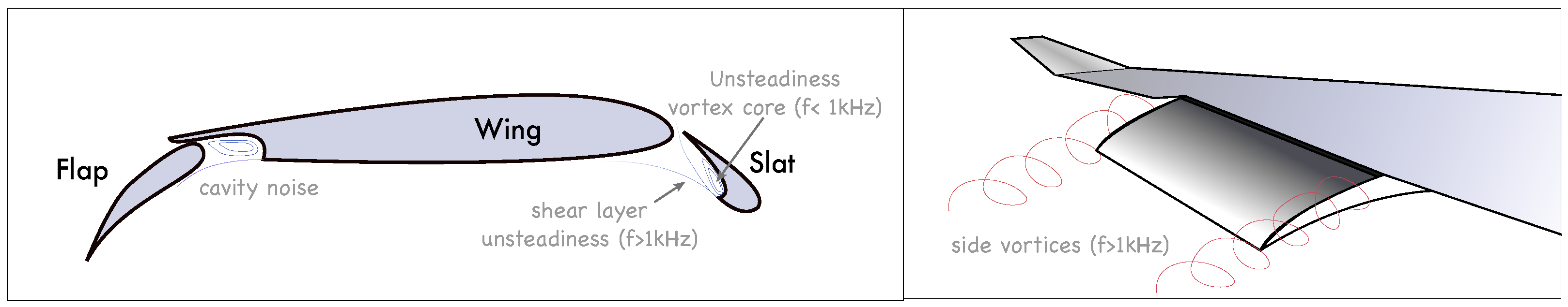
Slat noise. For the slat, two main mechanisms of noise were noted [19,45], see Figure 2. Low-frequency oscillations (below 1 kHz) arise due to the unsteadiness of the separation bubble which occurs behind the slat. A higher-frequency noise arises due to the unsteadiness in the shear layer. The aeroacoustic noise remains very sensitive to the geometry of the slat; minute changes to the geometry can modify the acoustic directivity [46]. The slat noise is often characterized by a tonal peak in the mid-frequency range and a broader bump in the low-frequency range [45,47]. Recent experimental work [47] explained the mechanisms of the tonal features of slat noise.

Flap noise. Flap noise has multiple physical origins. One of the important noise sources comes from the attached vortices on the side-edge of the flap, see Figure 2. The vortices initially contribute to high-frequency noise ($f>1$ kHz) but eventually merge and have a lower frequency contribution ($f<1$ kHz) [19]. Other works, such as Brooks and Humphreys [48], have also focused on flap noise. Their work noted that geometric features of the flap can impact the directivity pattern for low- and high-frequency ranges. A number of works have proposed models for flap noise, e.g., [49]. Salas et al. [50] compared high-lift noise estimation from analytical models to direct noise computations.

Landing gear noise. There are two dominant types of noise for landing gears. First, a broadband noise is generated from the shear layers, wakes and flow separation about the components of the landing gear such as the wheels or strut. The frequency range caused by these components is generally below 1 kHz. Secondly, tonal noise is generated from all cavities and openings. For modeling purposes, the broadband contributions are often of greater interest [19]. The scaling of the landing gear noise is of specific importance, and many works report a 6th or 7th power law of the landing gear noise emission energy with the velocity [51]. Recent works provide evidence that lower frequencies have a 6th power scaling while higher-frequencies collapse better with a 7th power scaling [52]. These scaling laws are particularly relevant given the large geometric variability among the various landing gears.

2.2. Propulsion Systems

The survey of propulsion system noise includes both jet engines and propellers. For the jet engines, we distinguish between the various sources of noise within the engine.

2.2.1. Jet Propulsion Noise

Jet exhaust noise. Historically, jet noise has played a significant role in the overall acoustic signature of aircraft. Yet, with increased acoustic shielding from the large bypass ratios, the importance of jet noise has been reduced. Jet noise is a distributed noise source that occurs primarily due to turbulent mixing in the jet. Many strategies have been developed for noise mitigation, including the addition chevrons [53] or mixing-ejectors. In high-speed jets, intermittent crackle noise, broadband shock-associated noise, and screech are important to the overall sound pressure level of the jet; a recent review of high-fidelity modeling of jet noise was completed by Bres and Lele [54]. The screech has a very distinct tonal characteristic and was the subject of a comprehensive review [55].

Engine noise. As a result of the jet noise mitigation strategies, engine noise has gained in importance. The engine noise is generated from various components of the jet engine. A review by Ihme [15] summarizes the contributions of each of these components. The compressor will generate noise from inflow distortions and turbulence as well as trailing edge shedding on the blades. The turbulent combustion within the combustor will generate direct noise through the unsteady local expansion of the gas, whereas the turbine and nozzle exhaust can generate indirect noise through compositional, entropy, and pressure perturbations that advect through throats or flow constrictions. Engine noise can have both tonal frequencies that emerge from the periodic blade passing frequency (at its harmonics) of the fan and compressor blades, and broadband characteristics. It should be noted that the interaction of the tonal features with the turbulence and shear layers may result in distortion and a broadening of the spectral peaks. At the sub-component scale, direct noise has historically been of key importance, but evidence of the importance of indirect noise considerations is increasing [56]—although, it should be noted that the importance of indirect noise has been recognized by many years [57,58]. Recent works have advanced the field of indirect noise estimation to include compositional and multi-stream effects [59,60,61,62,63].

2.2.2. Propeller Noise

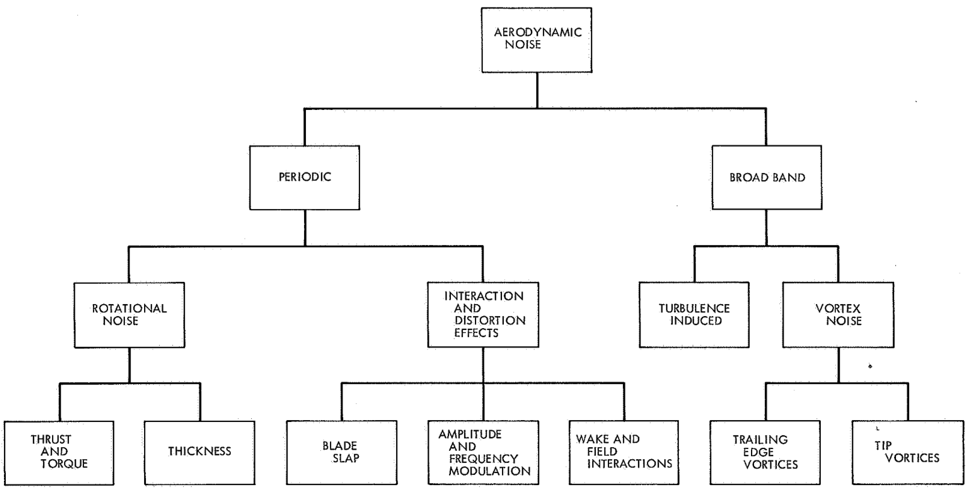
The propeller noise can be divided into three separate contributions, namely: harmonic, narrow-band random, and broadband noise [64]. The harmonic contribution, also the most distinctive, can be estimated from the number of blades B and the rotational speed N. The fundamental frequency is thus $BN$ from which the harmonic frequencies can be computed. The narrow-band noise is not perfectly periodic, and the spectra are spread out about the harmonic frequencies. Finally, broadband noise shows a well-distributed and continuous pressure spectrum. The discrete noise is characterized by the “thickness noise” and “loading noise”. The amplitude of the thickness noise is proportional to the displaced volume of air by the blade; the frequency is tied to the rotational speed and cross-sectional area of the blade. The loading noise is only important at high speeds and is the result of the pressure difference that arises due to the aerodynamic loading on the blades. A summary of the main acoustic sources can be seen in Figure 3. Some of the classical predictive models of propeller noise can be attributed to Farassat; the main derivations of the theory can be found in [65]. Propeller noise, given its distinctive tonal features, is increasingly relevant to drone acoustic detection [66]. The acoustic characteristics of these drones are actively being investigated by a number of groups, for example [67,68]. Given the generally lower Reynolds numbers of drones compared to traditional aircraft, additional issues may arise due to laminar separation, asymmetric wake formation [69], or transitional wakes [70,71], although the impacts on the aeroacoustic noise are not fully understood.

3. Acoustic Features of Wing Tip Vortices

Aerodynamic lifting surfaces naturally have a large pressure difference that is necessary to sustain lift. As wings have a finite span, the pressure difference at the tip causes a counter-rotating pair of trailing vortices to form. The vortices pose a risk to following aircraft due to the strong downwash–especially during take-off and landing. As a result, regulators impose conservative separation standards to avoid these potential hazards. The conservative separation times limit airport capacity and results in wasted time and fuel.

The motivation in the present section is to review the acoustic characteristics of trailing wake vortices as they relate to their detection via passive acoustic means. Naturally, the understanding of the acoustics of the tip vortices is directly tied to their hydrodynamic features, which are reviewed for completeness.

3.1. Characterizing Wing Tip Vortices

The strength of wing tip vortices is directly tied to the circulation of the wake vortex (${\mathsf{\Gamma }}_0$), which is proportional to the aircraft mass and inversely proportional to the aircraft speed. Barbaresco and Meier [72] present a mathematical relation:

$${\mathsf{\Gamma }}_0=\frac{Mg}{\rho \frac{\pi }{4}VB}$$

(1)

where M, g, $\rho$, V, and B are, respectively: the aircraft mass, gravitational constant, density of the air, aircraft velocity, and wingspan. The factor of $\frac{\pi }{4}$ is used in the estimation of an elliptic lift distribution on the wing.

The separation between the vortex pairs on an aircraft can be approximated by $b_0=\frac{\pi }{4}B$, and their downward induced velocity can be approximated as ${\mathsf{\Gamma }}_0/\left(2\pi b_0\right)$ [72]. The evolution of the position of a representative point vortex pair of equal strength can be described using the Biot–Savart Law as performed by [73]. As the vortices approach the ground, complexities arise due to the presence of a solid wall [74].

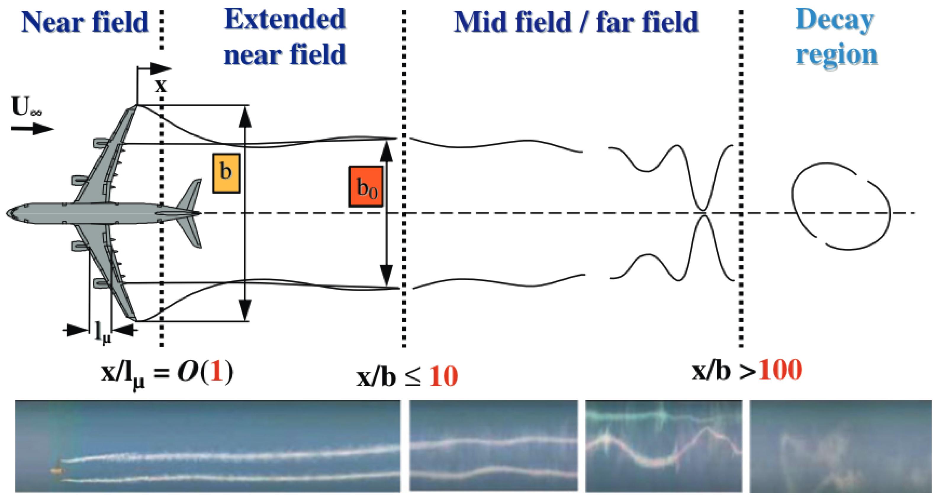
The life of a vortex can be divided into three phases [75]: the rollup, diffusion, and rapid decay. The rollup, in the extended near field, is characterized by the initial vortex sheet interaction, which occurs at $x<10B$ [40]. The diffusion phase occurs in the far field as the vortex grows and decays. This zone is also characterized by a self- and mutually-induced evolution of the vortices. Finally, if the vortex is not completely decayed from the diffusion phase, a rapid decay phase may occur in the presence of instabilities that can lead to reconnection, or vortex bursting. The primary linear instability mechanism in a counter-rotating vortex pair emerges due to symmetrical displacement of the vortex cores first explained by Crow [76], thus called the Crow instability. Under the symmetric core displacement, the vortices increase their mutual induction thus amplifying this linear instability until the vortex pair interacts. An illustration of the stages of the vortex life cycle is shown in Figure 4.

The size of the vortex core is an important quantity to define its aeroacoustic characteristics. Experimentally, it was determined by Delisi et al. [77] that the size of the vortex core, defined as the radial distance to the point of maximum tangential velocity, is on the order of 1% of the wingspan, although previous researchers suggested higher values [77].

High-fidelity simulations have provided a more detailed mechanism to understand the vortex decay in the atmosphere [75,78,79], as well as the Crow instability and subsequent reconnection [80]. The prediction of the vortex wake dynamics is greatly influenced by lower atmospheric weather–especially the wind. The trajectory and vortex decay in atmospheric turbulence were numerically investigated by Zheng and Li [78]. Furthermore, the self- and mutually-induced dynamics can result in Crow instability and cause vortex reconnection, which effectively precipitates the vortex decay. The multiple vortex interactions can shift the spectral peak of the newly merged vortices [81].

3.2. Analytical Vortex Flow

Typical vortex solutions, often presented as two-dimensional analytical equations, help represent the main features of an idealized vortex. A simplified vortex can be used to describe the tangential velocity [72]:

$$v_{\theta }\left(r\right)=\frac{{\mathsf{\Gamma }}_0}{2\pi r}\left(1-{\mathrm{e}}^{-g(r/B)}\right)$$

(2)

where r, ${\mathsf{\Gamma }}_0$, and B represent the radial position, the total circulation, and the wingspan of the aircraft. The definition of the function $g(r/B)$ depends on the type of vortex model. We can assume the radial velocity to be null or very small relative to the tangential velocity. Other analytical vortex solutions such as the Oseen–Lamb or Taylor vortex better account for the viscous core [82], but the simplicity of the above model is often preferred for analytical tractability. Some researchers, for example [83,84], use a Kirchoff vortex, characterized by an elliptical vorticity patch, as it enables them to model the proposed noise emission from the rotation of the vortex core. A comprehensive review of analytical vortex models was performed by Ahmad et al. [85].

The hydrodynamic pressure field is an important feature of the vortex. It should be noted that the hydrodynamic pressure does not propagate as an acoustic wave and it is therefore not directly perceived by the microphone array unless the vortex directly interacts with it. The hydrodynamic pressure field about an idealized point vortex can be defined as:

$$p=p_{\infty }-\frac{{\rho }_{\infty }{\mathsf{\Gamma }}_0^2}{8{\pi }^2{r}^2}$$

(3)

where r is the radius to the point vortex and the subscript ${}_{\infty }$ corresponds to the freestream state. Pressure distribution of more complex vortex models can be found in, for example, [82].

3.3. Acoustic Models for Vortex Sound

In order to use passive acoustic methods to detect and localize wake vortices, pressure fluctuations must propagate from acoustic sources in the vortex. Wake vortices have been shown to emit noise. The wake vortices were successfully identified using their acoustic emission captured on a phased array in a number of test campaigns, including at Berlin’s Airport Schönefeld [86] and Denver International airport [35,87,88]. The exact sources and mechanisms of aeroacoustic noise from the vortex remain subject to debate, but Hardin and Yang [73] noted the following likely sources:

• Core vibrations are excited by initial conditions or instabilities;
• Unsteady transport of the vortex, including possible interactions with secondary vortices, shed from the atmospheric boundary layer;
• Vortex core motion is excited by intermittent turbulent structure;
• Unsteady advection of turbulence around the vortex core.

Some works, such as Tang and Ko [89], suggest two main sound generation mechanisms, namely: vortex centroid dynamics and vortex core deformation. It is claimed that the vortex core deformation is responsible for a higher frequency peak compared to the centroid dynamics. Zheng et al. [83] studied an analytical Kirchoff vortex—a prototypical elliptical vortex—and proposed that the self-induction within the vortex core could result in a core rotation whose frequency aligns with the dominant frequency measured experimentally. Using data from the Denver experiments, they proposed an inverse relationship between the dominant frequency and the wing span, which is only valid for large aircraft. Zhang et al. [90] developed an analytical model and proposed that the acoustic signature during the wake vortex roll-up has a broadband feature with larger sound pressure levels in the sub 100 Hz range. When considering ground effects, Alix et al. [91] noted a broadband noise ranging from below 100 Hz to over 2000 Hz.

Although Zheng’s work proposed a mechanism for sound generation in a vortex, often simpler models are used to compute the vortex sound. From a fundamental point of view, the governing equations of the acoustic propagation, as well as the acoustic sources can be derived. Lighthill [92] derived a wave equation by combining the continuity and momentum equations under the assumption of a static medium. The homogeneous part represents a hyperbolic wave equation, while the right-hand are the acoustic source terms.

$$\frac{{\partial }^2\rho }{\partial t^2}-c_0^2{\nabla }^2\rho =\underset{\mathrm{S}}{\underbrace{\nabla ·\left[\rho (v·\nabla )v-v\frac{\partial \rho }{\partial t}+(\nabla p-c_0^2\nabla \rho )-\nabla ·\tau \right]}}$$

(4)

where $v$ is the velocity (vector), $c_0$ is the constant speed of sound of the stationary medium, and $\tau$ is the stress tensor. Recent work by Daryan et al. [93] recast the source terms into physically meaningful terms and investigated the individual contribution of each of those terms during the vortex evolution and reconnection. Lighthill’s equation, sometimes written in terms of pressure instead of density, serves as the basis for simpler acoustic models for vortex sound.

Starting from Lighthill’s equation, Powell [94] proposed a simple vortex sound model based on the divergence of the Lamb vector:

$$\frac{1}{c_0^2}\frac{{\partial }^{2}p}{\partial t^2}-{\nabla }^{2}p\approx \rho \nabla ·\left(\omega \times v\right)$$

(5)

where $\omega$ represents the vorticity vector. This equation is derived under an inviscid assumption and with the understanding that terms such as the gradient of the kinetic energy are negligible [95]. The above equation admits an analytical solution that can be used to propagate a pressure fluctuation to the far field, as performed by [96]. Using a similar starting point, Möhring derived an approximate acoustic model for an acoustically compact, vortical flow. The derivation of the equation using asymptotic expansions can be found in the appendix of [95]. The computational expense of Möhring’s solution is significantly reduced compared to Powell’s equation but shows an over-prediction compared to direct numerical simulation of the far-field noise [95]. A comprehensive review of vortex sound models can be found in [97].

3.4. Spectra of Vortex Wake Acoustics

The spectral features of the acoustics of the vortex wake are central to their identification. As mentioned earlier, Zheng et al. [83] proposed an inverse relationship between the dominant frequency and the wing span. Other researchers proposed that the dominant frequency of a wing tip vortex, which is tied to the rotation frequency of vortex cores, can be related to the circulation and the core radius [40]. They proposed that the peak frequency of vortex sound to be:

$$f\approx \frac{{\mathsf{\Gamma }}_0}{{\left(2\pi r_c\right)}^2}$$

(6)

where $r_c$ is the core size, which is a difficult quantity to estimate and varies significantly in the literature (see discussion and citations in [77]). Böhning et al. [40] tabulated the estimated peak frequencies for a number of aircraft. They found that the peak frequency is on the order of O(1 Hz) if we assume that the vortex core is 6% of the wingspan, whereas the peak frequency varies from 50–80 Hz if we assume that the vortex core is 1% of the wingspan. The latter estimates align better with the measured acoustic signal. In a later work, it was found that the dominant acoustic frequencies in the wake are not strongly influenced by the variation of the core size nor by the distance between the vortices [78]. As the vortices evolve, the core size increase remains modest. Therefore, the shift in frequency of the peak noise will be primarily tied to the decay of the circulation of the vortex [40].

As part of the European C-Wake, a number of experimental tests were conducted and summarized in the technical report by Böhning et al. [40]. Two systematic peaks are observed; the second, at about $f\approx O\left(100\mathrm{Hz}\right)$, is tied to the vortex sound. The first peak at $f\approx O\left(10\mathrm{Hz}\right)$ is unexplained. The measured power spectral density of the wake of a number of aircraft were investigated at various times during the wake evolution. Sample results of the power spectral density of the wake vortex noise can be found in [40].

More recently, using highly sensitive infrasonic microphones, Zuckerwar et al. [98] reported the identification of aircraft wakes using the coherence of their infrasonic signatures among a microphone pair. Similar infrasonic noise was measured a decade earlier by Rubin [39]. The infrasonic signature of the wake vortices is relevant for passive acoustic detection as low-frequency acoustic waves can propagate long distances with minimal attenuation and can be used to identify shuttle launches or clear-air turbulence [99].

3.5. Acoustic Features in the Decay Region

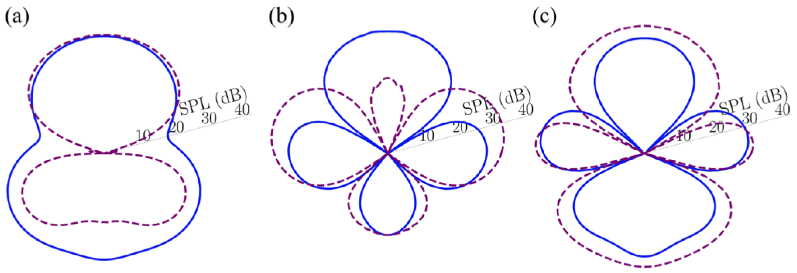
Under strong self and mutual interaction, the vortex pair may undergo a rapid decay resulting from a bursting event or, due to Crow instabilities, some form of viscous reconnection. The acoustic characteristics are not as well understood in this region. In recent works, Daryan et al. [93,100] characterized the resulting aeroacoustic noise from the reconnection of two anti-parallel vortices. Their analysis revealed the decidedly dipole-to-quadrupole sound pattern in the far-field during the reconnection. The acoustic sources migrate from the reconnection plane to the bridge as reconnection advances. Figure 5 shows the evolution of the sound pressure level during the reconnection. In a subsequent work, Daryan et al. [93] showed that the reconnection event caused a very rapid spike in the overall sound pressure level, which was attributable to a number of acoustic sources but, most notably, due to the flexion product.

4. Sound Propagation through the Atmosphere

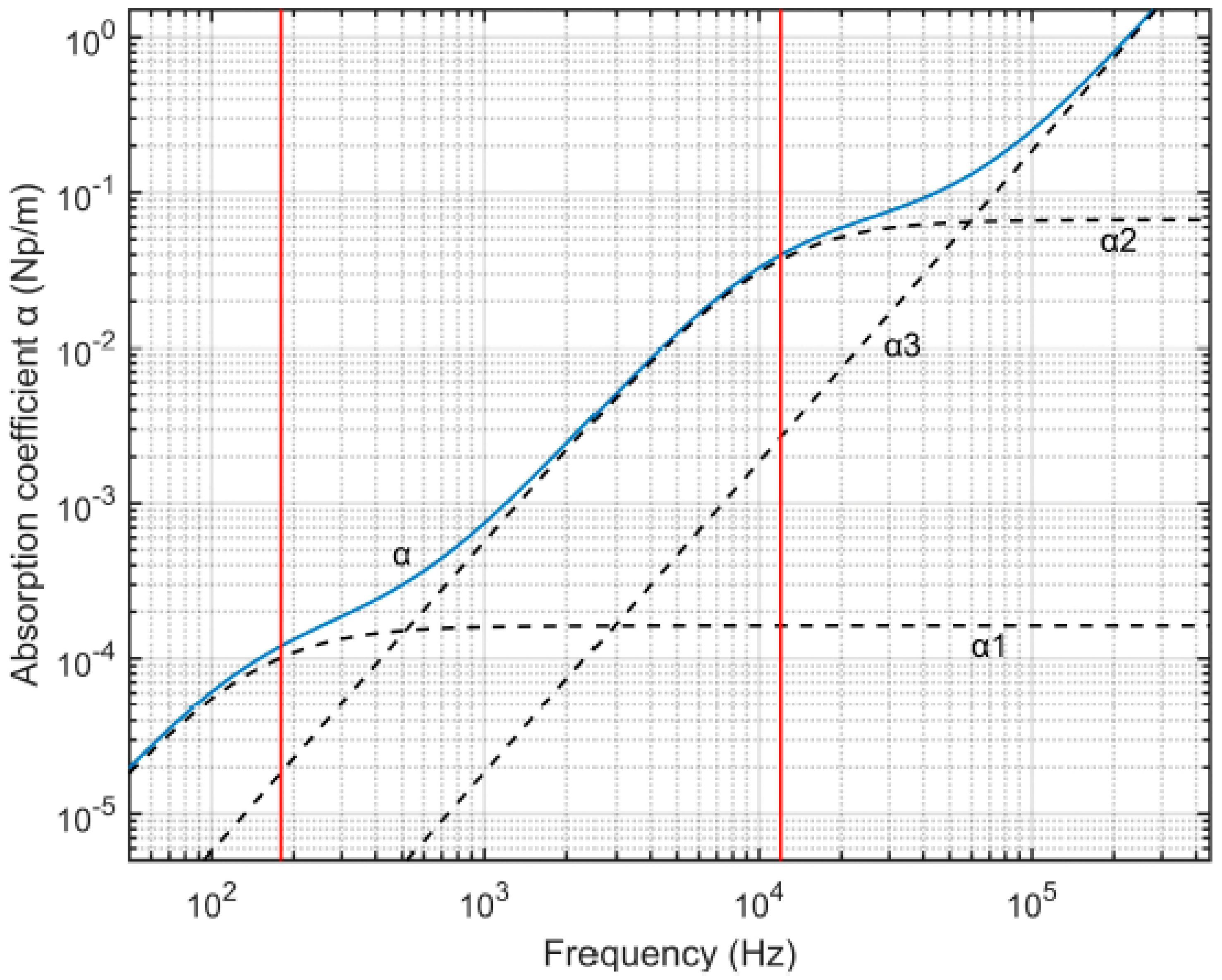
In order for a passive acoustic detection method to function, the acoustic signal needs to propagate between the source (aircraft or wake) and the receiver (microphone) while undergoing minimal loss. Generally, losses in the acoustic signal are tied to either geometric effects or atmospheric losses [101]; a modern treatise on modeling of atmospheric noise propagation can be found in [102]. Geometric losses are the result of the spreading of acoustic energy as the wavefronts expand, usually spherically, from a monopole source, which is often used to approximate an acoustic source. The atmospheric losses include the combined effects of absorption—due to viscous and molecular relaxation effects—and wind or temperature gradients in the atmosphere. The exponential attenuation of the acoustic noise through the atmosphere is frequency dependent, and modeling strategies are well established within international standards (see, for example [103]). The frequency dependence of the attenuation factor, at given atmospheric conditions, can be seen in Figure 6. As the low-frequency sound has orders of magnitude lower acoustic absorption coefficient, it can travel large distances compared to higher frequency sound. If the propagation distance through the atmosphere is large—which is only relevant to low-frequency sound—additional dispersion considerations due to the changing speed of sound in the atmosphere must be considered. The infrasonic range, often defined as frequencies below 20 Hz, is relevant for the identification of wing tip vortices but can also be used to identify other infrasonic generating noise sources such as tornadoes [104] or clear-air turbulence [99]. Often, undesirable low-frequency noise due to wind shear, for example, must be mitigated through the use of screens [105]. The celerity of the wave is tied to the isentropic compressibility of the medium; in air, this is primarily a function of the temperature, thus elevation. The finite propagation speed of acoustic waves—which is about 345 m/s at sea level at 20 °C and slightly under 300 m/s at cruising altitude.

5. Acoustic Source Localization

Acoustic localization refers to computing the angles (azimuth and elevation) describing the direction of arrival (DOA) of an acoustic source or finding its three-dimensional (3D) position using a microphones [6]. Passive acoustic localization techniques rely on the acoustic pressure signal measured from a single or an array of microphones to reconstruct the position of the detected acoustic source. Passive acoustic source localization techniques have a long history—especially for military applications—and are increasingly used in a number of civilian aerospace applications. Chen and Zhao [107] developed the mathematical formulation for locating low altitude and ground-moving targets using a small acoustic sensor array. Ref. [108] proposed a new localization method based Doppler-shifter passive acoustic detection methodology with a distributed microphone array. More recently, Sedunov et al. [37] presented a passive aircraft detection system specifically for the tracking, and classification of low-flying aircraft (LFA), which are frequently used for illicit activities. The system employs a network of passive acoustic sensors containing microphone clusters, cameras, and electronics. All these elements work cohesively to find the direction of arrival (DOA), localise the aircraft using triangulation, and then capture images. Harvey and O’Young [109] investigated the use of passive acoustic sensing as a collision avoidance technology for UAVs. Anti-collision systems are important for the safe operation of Unmanned Aerial Vehicles (UAVs) in populated airspace. Blanchard et al. [6] exploited the characteristic, harmonic nature of the acoustic signals generated by UAVs for their detection using a microphone array. Tong et al. [110] employed a Doppler-effect based method to estimate the closest point of approach, speed, direction of arrival, and other flight parameters of low-altitude flying aircraft using a stationary microphone array. Similarly, Ferguson [38] and Lo and Ferguson [111] used this same idea to estimate the motion parameters of propeller-driven aircraft. Piet et al. [112] carried out noise source localization on an aircraft using a large phased array of dimensions 16 m × 16 m consisting of 161 microphones. Tracking of moving sources using a ground-based array is complicated by Doppler frequency-shift and the variable amplitude of the signal received which happens as a result of the variable source-microphone distance during the aircraft flyover. Both these effects were countered by de-Dopplerization and normalization of the received microphone signals. Hafizovic et al. [113] used a circular, low-cost microphone array for acoustic detection and tracking of aircraft as part of a Runway Incursion Avoidance System (RIAS). It combines the array with the high-resolution Capon beamforming algorithm for real-time detection and tracking of aircraft. Acoustic tracking can potentially overcome the complexity, cost, and weather resilience challenges of RADAR-based systems. This review will focus on the main acoustic source identification techniques based on beamforming and review some modern approaches using machine learning techniques. But first, some theoretical considerations will be presented for completeness.

5.1. Theoretical and Experimental Considerations

Often, acoustic sources will be modeled using an idealized noise source. In aeroacoustics, most of the complex sources can be considered to be composed of a combination of monopole, dipole, and quadrupole sources. The typical noise sources are described in this section.

5.1.1. Noise Sources

Monopole

A monopole source radiates sound radially in all directions. An example of a monopole source would be a sphere whose radius expands and contracts sinusoidally. The acoustic pressure expression for a monopole source is a function of radial distance (r) from the center of the monopole and is given as [114]:

$$p(r,t)=i\frac{Q\rho ck}{4\pi r}{e}^{i(\omega t-kr)}$$

(7)

The pressure amplitude is then given as:

$$\begin{array}{c}\hfill \left|p\left(r\right)\right|=\frac{Q\rho ck}{4\pi r}\end{array}$$

where, Q is the complex source strength, $\rho$ is the fluid density, c is the speed of sound, k is the wave number given by $k=\frac{2\pi }{\lambda }$, and r is the distance from the source to the observation point.

Dipole

Two monopoles of equal strength but opposite phase, separated by a small distance d, make up a dipole. The expression for pressure radiated is [114]:

$$p(r,\theta ,t)=-i\frac{Q\rho c{k}^{2}d}{4\pi r}cos\left(\theta \right)e^{i(\omega t-kr)}$$

(8)

The amplitude of this wave is given as:

$$\begin{array}{c}\hfill \left|p(r,\theta ,t)\right|=\frac{Q\rho ck}{4\pi r}kdcos\left(\theta \right)\end{array}$$

All the terms are the same as before, except for $\theta$. Unlike a monopole, a dipole does not radiate equally in all directions; its directivity depends on the angle, $\theta$, from the center of the dipole.

Quadrupole

A quadrupole source is composed of two identical dipoles with opposite phases separated by a small distance D, which is defined as the distance between the centers of the two dipoles arranged in either lateral or longitudinal configuration. The distance between the two monopoles making up a dipole is denoted by d. For longitudinal configuration, the dipole axes lie along the same line, unlike in the lateral configuration. Just like a dipole, the directivity of a quadrupole source is a function of the angle $\theta$ from the center of the quadrupole. The sound pressure amplitude for a longitudinal quadrupole is given as [114]:

$$\left|p(r,\theta ,t)\right|=\frac{Q\rho ck}{4\pi r}4k^{2}dD{cos}^2\left(\theta \right)$$

(9)

Similarly, the sound pressure amplitude for a lateral quadrupole is given as:

$$\left|p(r,\theta ,t)\right|=\frac{Q\rho ck}{4\pi r}4k^{2}dDcos\left(\theta \right)\sin \left(\theta \right)$$

(10)

5.1.2. Acoustic Measurement and Transformation

Beamforming is a popular acoustic source localization method. It can be applied both in the time and frequency domain. Time-domain beamforming is generally used for moving sources while frequency-domain beamforming is used for the detection of stationary sources [8]. The microphone array and a data acquisition system are the most important components needed in acoustic beamforming. An array of M microphones is placed in the region where the source is to be detected. The signal is measured by the microphone membrane, thus producing an AC voltage proportional to the pressure. This signal, from each microphone, then goes through the data acquisition system wherein the continuous analog pressure signal $p\left(t\right)$ is converted to a discrete digital signal $p(n\Delta t)$ and stored in memory. Here, $\Delta t=1/f_s$ where $f_s$ is the sampling frequency and n is an integer. For further processing, the signal has to be transformed to bring it into the frequency domain. This is performed using the Fast Fourier Transform (FFT) algorithm [115,116].

5.2. Beamforming

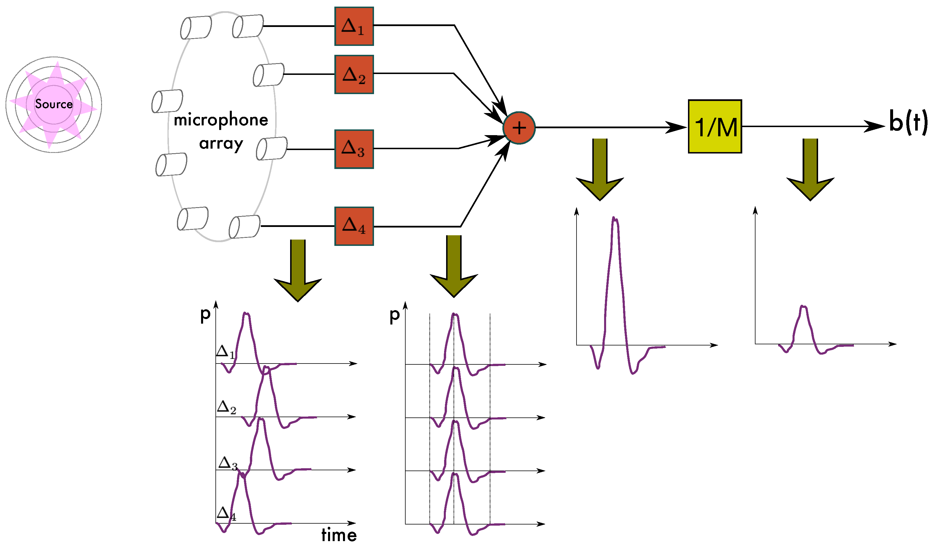
A phased microphone array is used for beamforming to identify the acoustic source. The array is steered or focused towards different points in space to check whether a source is present. When sound waves emanating from a source reach different microphones, there is a time delay with respect to the center of the array by virtue of different propagation distances. During processing, the amplitude and phase of the signals received by the microphones are modified to compensate for the delay such that constructive interference occurs if a source is present at the steered location. This suppresses the noise around the focal point while preserving the sound originating from the focal point [86]. By steering the array from one point to another of the assumed scanning grid in space, an acoustic source map is obtained. This is known as Delay-and-Sum beamforming [117] (Figure 7).

Source modeling is another important aspect of beamforming. As mentioned before, most of the complex source distributions in aeroacoustics can be considered to be composed of a combination of monopole, dipole, and quadrupole sources. Delay-and-Sum beamforming approach inherently assumes sources to be monopoles. Thus, the processing is based on the assumption that the sound waves emitted by the sources are spherical, and their amplitude is only a function of distance. Parameters such as source directivity, which would mean that the amplitude depends on the emission angle, do not play a role.

For an array of M microphones, delay-and-sum beamforming is given as [118]

$$b\left(t\right)=\frac{1}{M}\sum _{m=1}^M{w}_m{p}_m(t-{\mathsf{\Delta }}_m)$$

(11)

where $w_m$ is a weighting and ${\mathsf{\Delta }}_m$ is the time delay applied to the $m\mathrm{th}$ microphone.

The beamformer output in the time-domain as given by [116] is

$$L(t,x_0)=\frac{4\pi }{M}\sum _{m=1}^M{p}_m(x_0,t+t_0)|x-x_0|$$

(12)

where $p_m$ is the signal measured by each microphone, M is the number of microphones, $x_0$ is the source position and x is the microphone location.

In the frequency domain, the formulation differs slightly. Consider a microphone array being steered at an arbitrary location in space. The beamformer output of delay-and-sum beamforming in the frequency domain is given by taking the Fourier transform of the above beamformer equation as [116]:

$$L(\omega ,x_0)=F\left(z\left(t\right)\right)=\frac{4\pi }{M}\sum _{m=1}^M|x_m-x_0|P(x_m,x_0,\omega )e^{i\omega t_m}=\frac{1}{M}\sum _{m=1}^{M}s(x_m,\omega )P(x_m,x_0,\omega )$$

(13)

where, $P(x_m,x_0,\omega )$ is the Fourier transformed acoustic pressure of the source as measured by the $m\mathrm{th}$ microphone, and $s(x_m,\omega )=4\pi |x_m-x_0|e^{i\omega t_m}$ and $t_m$ are the steering function and the retarded time for that particular microphone. Since the array consists of M microphones, the steering function can be expanded into a steering vector $g(x,\omega )$ as:

$$\begin{array}{c}\hfill g(x,\omega )=\left(\begin{array}{c}4\pi |x_1-x_0|e^{i\omega t_1}\\ 4\pi |x_2-x_0|e^{i\omega t_2}\\ 4\pi |x_3-x_0|e^{i\omega t_3}\\ ⋮\\ 4\pi |x_M-x_0|e^{i\omega t_M}\end{array}\right)\end{array}$$

Here, the points $(x_1,x_2,x_3\cdots x_M)$ represent the microphone positions and $(t_1,t_2,t_3\cdots t_M)$ are the propagation times taken by the sound wave to travel from the grid point $x_0$ to the respective microphones. The acoustic pressure $P(x,x_0,\omega )$ detected by each microphone is written in the form of a combined pressure vector as:

$$P(x,x_0,\omega )=\left(\begin{array}{c}P(x_1,x_0,\omega )\\ P(x_2,x_0,\omega )\\ P(x_3,x_0,\omega )\\ ⋮\\ P(x_M,x_0,\omega )\end{array}\right)$$

(14)

The beamforming output at the steering location $x_0$ is given as:

$$L(\omega ,x_0)=\frac{g{(x,\omega )}^{H}P(x,x_0,\omega )}{M}$$

(15)

where $g{(x,\omega )}^H$ denotes the conjugate transpose of the steering vector $g(x,\omega )$. The mean squared power output of the beamformer is defined as:

$$Power=|L(\omega ,x_0){|}^2=L(\omega ,x_0)L{(\omega ,x_0)}^{*}$$

(16)

where $L{(\omega ,x_0)}^{*}$ denotes the complex conjugate of $L(\omega ,x_0)$. Since L is a scalar, $L^{*}=L^H$. So the expression for power is simplified as:

$$\begin{array}{cc}\hfill Power& =\frac{g{(x,\omega )}^{H}P(x,x_0,\omega )}{M}\frac{{\left(g{(x,\omega )}^{H}P(x,x_0,\omega )\right)}^H}{M}\hfill \\ \\ \hfill & =\frac{g{(x,\omega )}^H\left(P(x,x_0,\omega )P{(x,x_0,\omega )}^H\right)g(x,\omega )}{M^2}\hfill \end{array}$$

(17)

The term $P(x,x_0,\omega )P{(x,x_0,\omega )}^H$ is defined as the Cross-Spectral Matrix (CSM), which is a very important concept in beamforming and is defined as:

$$CSM=P(x,x_0,\omega )P{(x,x_0,\omega )}^H$$

(18)

Thus, we can define the power as:

$$Power=\frac{g{(x,\omega )}^H\left(CSM\right)g(x,\omega )}{M^2}$$

(19)

The beamforming power output is the spectral power output at the particular steering location. The power at all such scanning points is calculated by steering the array towards those points to generate an acoustic source map.

5.3. Machine Learning Approaches

Machine learning-based approaches have been used for acoustic source localization, which can be adapted for wake detection and tracking [119,120]. In particular, Deep Learning algorithms have emerged as powerful tools in a variety of disciplines over the years due to their ability to learn patterns and extract features from limited or unstructured data. Rapid growth in data and synthetic data generation techniques have added to their popularity. Deep learning algorithms can recognize and learn the patterns of microphone acoustic data obtained for various source distributions and then give accurate predictions for source positions and strengths when challenged with new microphone data.

Xu et al. [119] and Ma and Liu [120] proposed deep learning frameworks based on the principles of acoustic beamforming. A conventional technique, such as acoustic beamforming, is a common method for obtaining spectral information about the wake of acoustic sources. It makes use of phased microphone arrays, which are capable of suppressing the background noise and giving a reasonably accurate and clean source map. However, beamforming comes with its own set of limitations. The resolution of the source map is indirectly proportional to the frequency of the source, and thus beamforming suffers from spatial aliasing and poor resolution at lower source frequencies. Many of the recent works propose a deep learning framework that is able to perform well even at low source frequencies, and as a robust alternative method to acoustic beamforming.

The proposed deep learning framework is a data-driven method. In particular, Ma and Liu [120] uses a Convolutional Neural Network (CNN) for the detection of acoustic sources. A Convolutional Neural Network [121] is a type of neural network that finds its application extensively in image classification and segmentation. The network takes an image as input and tries to extract and learn its features. An image is essentially a matrix of pixel values, and thus any matrix that encapsulates the microphone data containing the acoustic pressure information of the sources can be used to train the network. The convolution layer applies a series of filters to the image that help the network capture the various features of the image. A filter is nothing but an array of numbers or weights that progressively goes over the image, calculating and storing the weighted sum of the pixel values. This also reduces the dimensions of the image. In the case of a typical image, a filter might help detect the vertical edges in the image by highlighting them and attenuating the other features, while another filter might help detect the horizontal edges, and so on. Multiple filters are used, and the resulting feature maps are stacked together.

The convolution operation is followed by pooling. The purpose of pooling is to downsample the image to reduce its dimensions and complexity while preserving the dominant features. Generally, Max-pooling is used [121]. It breaks down the image into rectangles of a specified dimension and stores the maximum of the pixel values that fall within each rectangle. Once the convolution and pooling operations are performed, the final image is flattened into a fully-connected layer and fed to a regular feed-forward neural network. The most important advantage of a CNN is the significant reduction in the number of parameters and computational requirements as compared to a regular Artificial Neural Network (ANN).

The CNN requires image data for training and validation. Since these frameworks are based on the principles of beamforming, they use the beamforming algorithm for generating synthetic data to train the network. As in beamforming, the sound sources are modeled as monopoles and radiate spherical pressure signals. The complex pressure signal in the frequency domain from a source s on the scanning grid to a microphone m on the array plane is given as [119]:

$$P_s\left(m\right)=\frac{e^{-i2\pi f{r}_s/c_0}}{4\pi |r_s|}$$

(20)

where $r_s$ is the distance between the particular source s and the microphone m and $c_0$ is the speed of sound in air. In beamforming, the total pressure from all the sources is recorded by every microphone. Adding the pressure signals from all the S sources present on the scanning grid at every microphone, the pressure vector P is obtained as:

$$P=\left[\begin{array}{ccc}\sum _{s=1}^S{P}_s\left(1\right),& \sum _{s=1}^S{P}_s\left(2\right),& \sum _{s=1}^S{P}_s\left(3\right),\cdots ,\sum _{s=1}^S{P}_s\left(M\right)\end{array}\right]$$

(21)

The Cross-Spectral Matrix (CSM) can be defined as in Equation (18). Ma and Liu [120] used the Cross-Spectral Matrix, which has dimensions of M × M as an input to the CNN. The network trains against the ground truth, which is a matrix containing the actual source location data from which the Cross-Spectral Matrix has been derived.

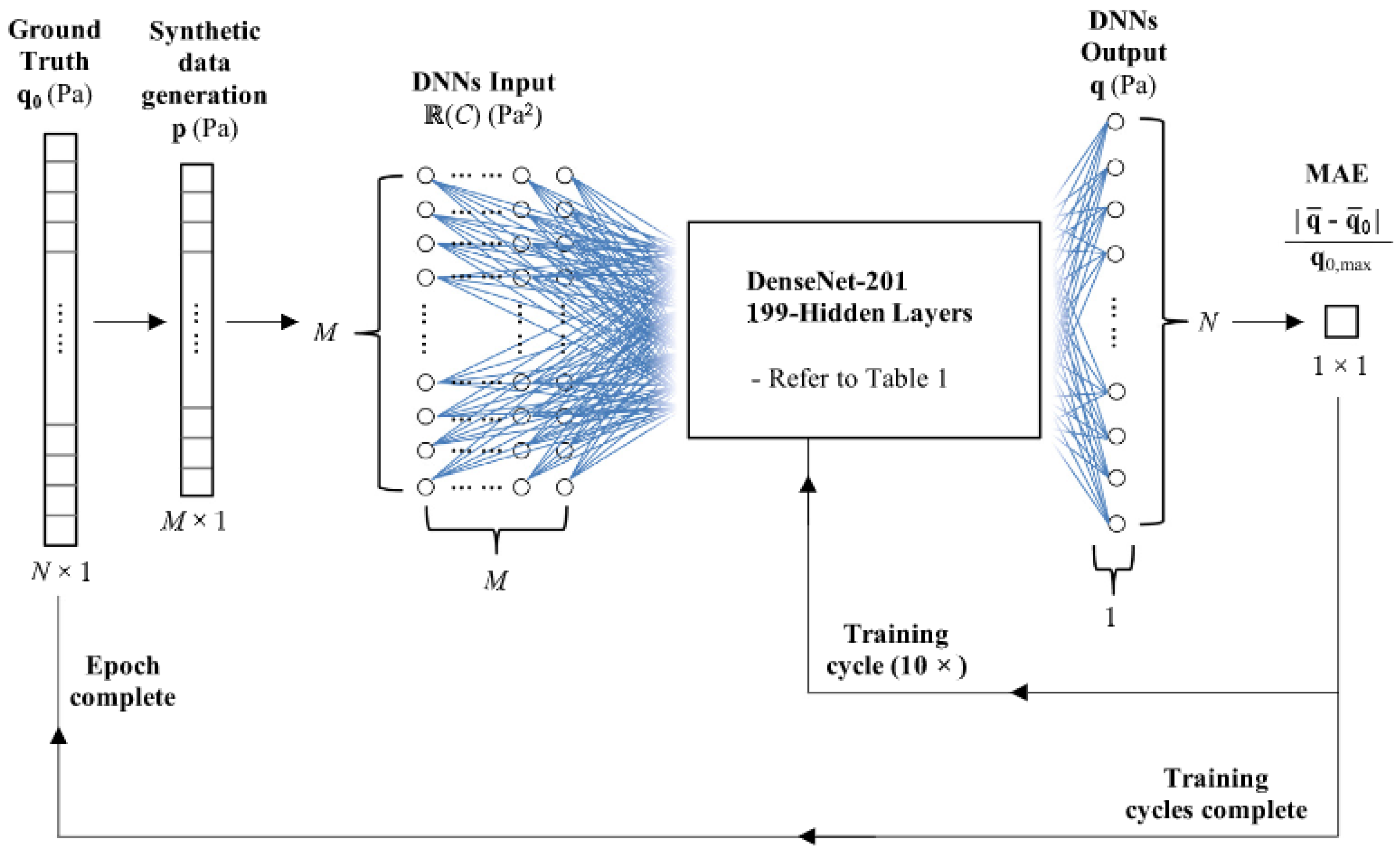
Xu et al. [119] used a sophisticated Deep Neural Network (DNN) model known as the Densely Connected Convolutional Network [122] (DenseNet) for acoustic source imaging. DenseNet possesses an advantage over other DNN architectures such as ResNet. It contains multiple Dense Blocks, which in turn contain multiple densely connected convolutional layers. These Dense Blocks are connected by transition layers that do convolution and pooling. DenseNet ensures maximum possible information flow between the layers. The number of parameters during training and computation are also reduced. For these reasons, Xu et al. [119] used the DenseNet-201 architecture (where 201 denotes the number of layers in the network). They simulated a virtual 64-channel microphone array, capturing the acoustic source distribution data from a scanning grid located 1.2 m above the array plane. The scanning plane of 1 m × 1 m was divided into a scanning grid. Monopole acoustic sources were simulated randomly across the scanning grid. The real part of the Cross-Spectral Matrix was used as an input feature, and the network’s prediction was compared against the ground truth (Figure 8).

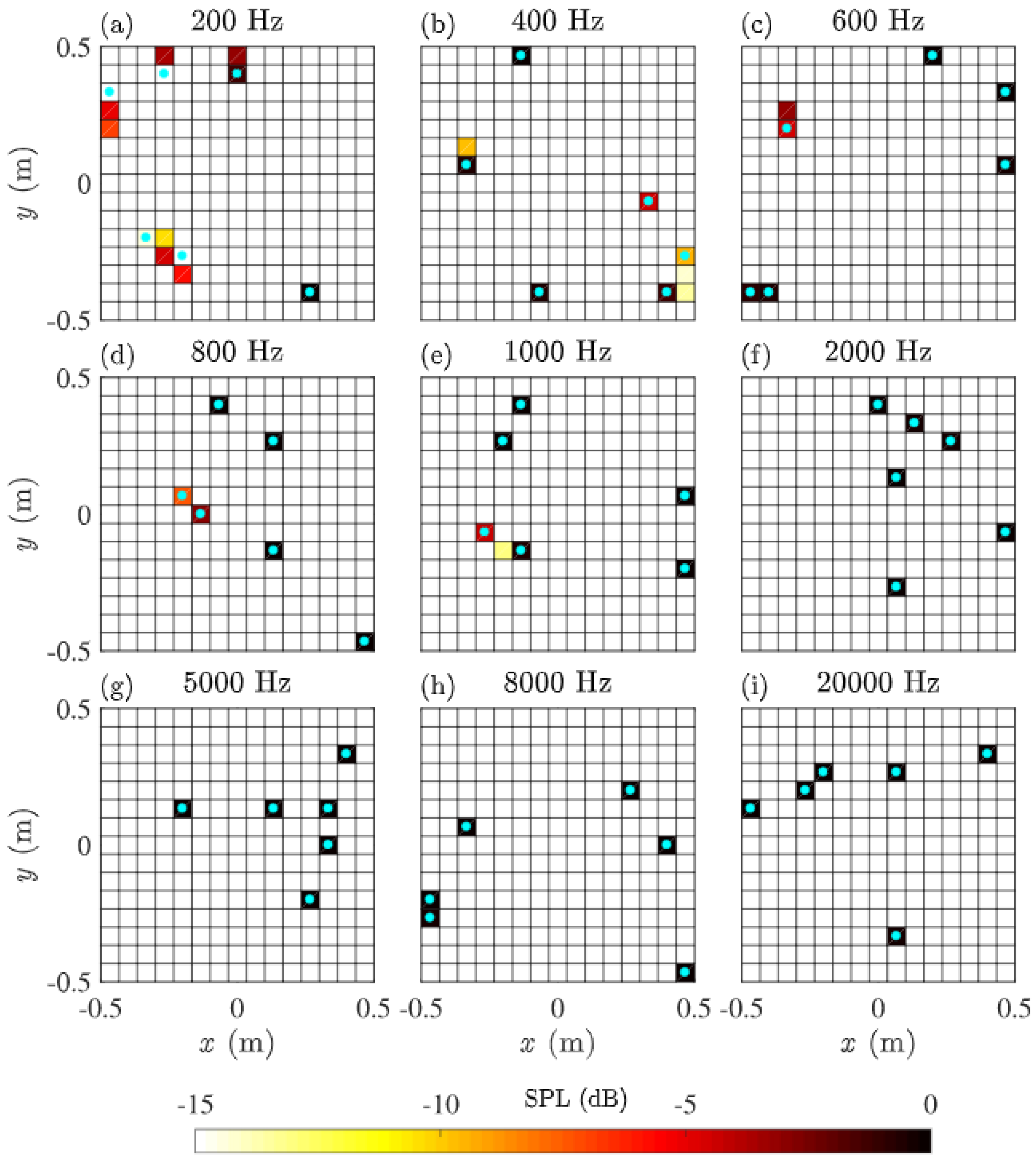
Wake acoustic sources lie in the frequency bands between 100 Hz and 500 Hz, as established by the Denver Airport Test [35], and possibly at lower frequencies. Multiple DenseNet models were developed that were trained to detect a fixed and random number of sources at frequencies ranging from 100 Hz to 20,000 Hz. The network was able to resolve complex source distributions, and while it naturally performed much better at higher frequencies, its performance at low frequencies is what separated it from classical beamforming. Figure 9 shows the DenseNet performance at various frequencies. The DenseNet was trained to detect 6 sources of equal strength, distributed randomly across a 15 × 15 scanning grid. Frequencies between 200–800 Hz are generally considered relatively low for beamforming, but the network was able to locate every source from 400 Hz onwards and also give a reasonably accurate representation of the ground truth for lower frequencies. Future work involves building a more robust and generalized model capable of detecting a variable number of sources for a range of frequencies.

Other Works

The machine learning approaches have also been adopted for non-acoustic detection methods. Weijun et al. [123] has developed a deep learning based object detection algorithm based on the Doppler LIDAR detection principle. Their results have shown that the algorithm can facilitate the LIDAR based technique in high-confidence aircraft wake detection and improve the decision-making and aircraft safety.

Doppler LIDAR transmits pulses of infrared laser light in the airspace being scanned. Atmospheric molecules and aerosols scatter some portion of the light back to the receiver. The received frequency is Doppler-shifted by $\mathsf{\Delta }{f}_D$ due to the random motion of the atmospheric particles. The velocity field of the wake vortex can be obtained from the relation between the calculated Doppler shift and the radial velocity of the wake vortex ($V_R$):

$$\mathsf{\Delta }{f}_D=\frac{2f_{0}V}{C}=\frac{2}{{\lambda }_0}{V}_R$$

(22)

where $f_0$, ${\lambda }_0$, and C are the emitted frequency, wavelength, and speed of light, respectively.

Once the velocity field has been obtained, the target detection algorithm is applied. The YOLO algorithm is used, which stands for You Only Look Once. YOLO [124] is a type of convolutional neural network that is used for single-step target detection. The network is trained to detect a fixed number of objects that are enclosed by bounding boxes. The image is divided into a grid. For each grid, a prediction vector for each bounding box containing 5 parameters is defined. These parameters are $(x,y,w,h,c)$. Here, $(x,y)$ is the center point position of the object, w and h are the width and height of the bounding box respectively, and c is the confidence of the target. The prediction vectors for all the B bounding boxes are concatenated to generate one large vector which the network uses to train itself against. The experimental results showed that the model could detect the wake from the LIDAR’s results with an accuracy of around 94% Weijun et al. [123].

Quaranta and Dimino [125] used an Artificial Neural Network (ANN) to identify different types of aircraft based on their acoustic signature. For training the network, they employed a wavelet-based decomposition of the aircraft noise signals. This was followed by a feature extraction process that involves statistical analysis of the wavelet coefficients and the evaluation of the energy content of each wavelet decomposition level. The process ultimately yielded feature vectors corresponding to each aircraft type that could then be used to design and train a neural network.

6. Conclusions

This work presents a modern bibliographic review of the state of knowledge in the fields of aeroacoustic noise and acoustic-based detection methods for aerospace applications. The objective of this work is to advance the field of passive acoustic detection by combining knowledge from these two distinct fields into a single review paper. Despite being an established technology with decades worth of practical knowledge, passive acoustic-based detection is increasingly being explored for novel applications—especially for UAVs. Acoustic-based methods display clear advantages in terms of cost and weight which makes them particularly well-suited for on-board detection in smaller vehicles. Recent works by companies such as Zipline [126] are leveraging acoustic microphones for onboard collision and avoidance systems. In parallel, a growing number of companies such as XWing [127] and Ribbit [128] are developing pilotless aircraft for which passive acoustic-based methods can potentially be integrated, most notably as a redundant safety system.

In this work, a timely review of the characterization of aircraft aeroacoustics is presented with a focus on the main noise sources, their spectral characteristics, and dominant sound generation mechanisms that are relevant to passive acoustic detection methods. The main focus was placed on passenger planes which cover a broad spectrum of frequencies. Smaller UAVs and drones, have decidedly different acoustic features which were only briefly reviewed in the current paper but should be the focus of future review works on this topic. Section 3 summarizes the state-of-the-art in vortex and wing tip noise characterization. Although acoustic detection methods have been applied to locate these wing tip vortices, the physical mechanisms of noise generation remain plagued with some uncertainty. There is consensus on the importance of the circulation and core radius, but the characterization of the core radius, in particular, remains challenging. Given that the circulation of the tip vortices are proportional to the mass of the aircraft, this section may not be applicable to smaller vehicles such as drones. Section 4 briefly covers the important considerations for the sound propagation through the atmosphere, and highlights the long-distance propagation and low attenuation of infrasonic sound. The long-distance propagation of low-frequency noise, often in the infrasonic range, presents many advantages in aircraft tracking, especially for outside the line-of-sight but again may only be applicable to larger aircraft. Finally, in Section 5, we review the main concepts related to the acoustic source localization with a specific focus on beamforming and modern machine learning approaches. The main disadvantage of beamforming lies in the difficulty of low-frequency source localization. Neural network-based techniques have largely overcome this challenge, which provides new opportunities for wing vortex localization. With the ongoing success and strengths of the machine learning approaches, it is anticipated that much of the advances in passive acoustic detection algorithms will utilize emerging technologies.

References

- Casalino, D.; Diozzi, F.; Sannino, R.; Paonessa, A. Aircraft noise reduction technologies: A bibliographic review. Aerosp. Sci. Technol. 2008, 12, 1–17. [Google Scholar] [CrossRef]
- Ju, S.; Sun, Z.; Guo, D.; Yang, G.; Wang, Y.; Yan, C. Aerodynamic-Aeroacoustic Optimization of a Baseline Wing and Flap Configuration. Appl. Sci. 2022, 12, 1063. [Google Scholar] [CrossRef]
- Piccirillo, G.; Viola, N.; Fusaro, R.; Federico, L. Guidelines for the LTO Noise Assessment of Future Civil Supersonic Aircraft in Conceptual Design. Aerospace 2022, 9, 27. [Google Scholar] [CrossRef]
- Stubbs, C.; Brenner, M.; Flatt, S.; Goodman, J.; Hearing, B. Tactical Infrasound. Intelligence 2005, 0515, 72. [Google Scholar]
- Schönhals, S.; Steen, M.; Hecker, P. Towards wake vortex safety and capacity increase: The integrated fusion approach and its demands on prediction models and detection sensors. Proc. Inst. Mech. Eng. Part G J. Aerosp. Eng. 2013, 227, 199–208. [Google Scholar] [CrossRef]
- Blanchard, T.; Thomas, J.H.; Raoof, K. Acoustic localization and tracking of a multi-rotor unmanned aerial vehicle using an array with few microphones. J. Acoust. Soc. Am. 2020, 148, 1456–1467. [Google Scholar] [CrossRef]
- Lykou, G.; Moustakas, D.; Gritzalis, D. Defending Airports from UAS: A Survey on Cyber-Attacks and Counter-Drone Sensing Technologies. Sensors 2020, 20, 3537. [Google Scholar] [CrossRef]
- Merino-Martínez, R.; Sijtsma, P.; Snellen, M.; Ahlefeldt, T.; Antoni, J.; Bahr, C.J.; Blacodon, D.; Ernst, D.; Finez, A.; Funke, S.; et al. A Review of Acoustic Imaging Methods Using Phased Microphone Arrays: Part of the “Aircraft Noise Generation and Assessment” Special Issue; Springer: Vienna, Austria, 2019; Volume 10, pp. 197–230. [Google Scholar] [CrossRef] [Green Version]
- Filippone, A. Aircraft noise prediction. Prog. Aerosp. Sci. 2014, 68, 27–63. [Google Scholar] [CrossRef]
- Isermann, U.; Bertsch, L. Aircraft noise immission modeling. CEAS Aeronaut. J. 2019, 10, 287–311. [Google Scholar] [CrossRef]
- Quaranta, V.; Dimino, I. A Method For Acoustic Signature Identification Of Aircraft. In Proceedings of the Twelfth International Congress on Sound and Vibration, Florence, Italy, 12–16 July 2015; pp. 1–10. [Google Scholar]
- Morinaga, M.; Mori, J.; Matsui, T.; Kawase, Y.; Hanaka, K. Identification of jet aircraft model based on frequency characteristics of noise by convolutional neural network. Acoust. Sci. Technol. 2019, 40, 391–398. [Google Scholar] [CrossRef]
- Bailly, C.; Bogey, C.; Marsden, O. Progress in Direct Noise Computation. Noise Notes 2010, 9, 31–48. [Google Scholar] [CrossRef] [Green Version]
- Bodony, D.J.; Lele, S.K. Current status of jet noise predictions using large-eddy simulation. AIAA J. 2008, 46, 364–380. [Google Scholar] [CrossRef]
- Ihme, M. Combustion and Engine-Core Noise. Annu. Rev. Fluid Mech. 2017, 49, 277–310. [Google Scholar] [CrossRef]
- Marte, J.; Kurtz, D. A Review of Aerodynamic Noise from Propellers, Rotors, and Lift Fans; Technical Report; Jet Propulsion Laboratory: Pasadena, CA, USA, 1970. [Google Scholar]
- Morfey, C.L. Amplification of aerodynamic noise by convection flow inhomogeneities. J. Sound Vib. 1973, 31, 391–397. [Google Scholar] [CrossRef]
- Peake, N.; Parry, A.B. Modern challenges facing turbomachinery aeroacoustics. Annu. Rev. Fluid Mech. 2011, 44, 227–248. [Google Scholar] [CrossRef]
- Molin, N. Airframe noise modeling and prediction. CEAS Aeronaut. J. 2019, 10, 11–29. [Google Scholar] [CrossRef]
- Moreau, S. The third golden age of aeroacoustics. Phys. Fluids 2022, 34, 031301. [Google Scholar] [CrossRef]
- Leylekian, L.; Lebrun, M.; Lempereur, P. An Overview of Aircraft Noise Reduction Technologies. AerospaceLab 2014, 1, 1–15. [Google Scholar]
- Hallock, J.N.; Holzäpfel, F. A review of recent wake vortex research for increasing airport capacity. Prog. Aerosp. Sci. 2018, 98, 27–36. [Google Scholar] [CrossRef]
- Zhou, J.; Chen, Y.; Li, D.; Zhang, Z.; Pan, W. Numerical simulation of aircraft wake vortex evolution and wake encounters based on adaptive mesh method. Eng. Appl. Comput. Fluid Mech. 2020, 14, 1445–1457. [Google Scholar] [CrossRef]
- Luber, W. Wake penetration effects on dynamic loads and structural design of military and civil aircraft. Conf. Proc. Soc. Exp. Mech. Ser. 2011, 3, 1381–1402. [Google Scholar] [CrossRef]
- Gerz, T.; Holzäpfel, F.; Darracq, D. Commercial aircraft wake vortices. Prog. Aerosp. Sci. 2002, 38, 181–208. [Google Scholar] [CrossRef]
- Michel, D.T.; Dolfi-Bouteyre, A.; Goular, D.; Augère, B.; Planchat, C.; Fleury, D.; Lombard, L.; Valla, M.; Besson, C. Onboard wake vortex localization with a coherent 15 µm Doppler LIDAR for aircraft in formation flight configuration. Opt. Express 2020, 28, 14374. [Google Scholar] [CrossRef] [PubMed]
- Breitsamter, C. Wake vortex characteristics of transport aircraft. Prog. Aerosp. Sci. 2011, 47, 89–134. [Google Scholar] [CrossRef]
- Rokhsaz, K.; Kliment, L.K. A Brief Survey of the Experimental Methods Used for Wake Vortex Investigations; SAE Technical Paper; SAE International: Warrendale, PA, USA, 2007; pp. 776–790. [Google Scholar] [CrossRef]
- George, R.; Yang, J.J. A Survey for Methods of Detecting Aircraft Vortices. In Proceedings of the ASME 2012 International Design Engineering Technical Conferences and Computers and Information in Engineering Conference, Chicago, IL, USA, 12–15 August 2012; DETC2012-70632. pp. 1–10. [Google Scholar]
- Georges, T.M. Acoustic Ray Paths through a Model Vortex with a Viscous Core. J. Acoust. Soc. Am. 1972, 51, 206–209. [Google Scholar] [CrossRef]
- Burnham, D.C. Characteristics of a wake-vortex tracking system based on acoustic refractive scattering. J. Acoust. Soc. Am. 1977, 61, 647–654. [Google Scholar] [CrossRef]
- Rodenhiser, R.J.; Durgin, W.W.; Johari, H. Acoustic technology for aircraft wake vortex detection. In Proceedings of the 86th AMS Annual Meeting, Atlanta, GA, USA, 29 January–2 February 2006; pp. 1–11. [Google Scholar]
- Llewellyn Smith, S.G.; Ford, R. Three-dimensional acoustic scattering by vortical flows. I. General theory. Phys. Fluids 2001, 13, 2876–2889. [Google Scholar] [CrossRef] [Green Version]
- Steen, M.; Schönhals, S.; Polvinen, J.; Drake, P.; Cariou, J.P.; Dolfi-Bouteyre, A.; Barbaresco, F. Candidate technologies survey of airport wind & wake-vortex monitoring sensors: Sensors for weather & wake-vortex hazards mitigation. In Proceedings of the 9th Innovative Research Workshop and Exhibition, INO 2010, Brétigny-sur-Orge, France, 7–9 December 2010; pp. 75–82. [Google Scholar]
- Booth, E.R.; Humphreys, W.M. Tracking and characterization of aircraft wakes using acoustic and lidar measurements. In Proceedings of the Collection of Technical Papers—11th AIAA/CEAS Aeroacoustics Conference, Monterey, CA, USA, 23–25 May 2005; Volume 3, pp. 2076–2101. [Google Scholar] [CrossRef] [Green Version]
- Sutin, A.; Salloum, H.; Sedunov, A.; Sedunov, N. Acoustic detection, tracking and classification of Low Flying Aircraft. In Proceedings of the 2013 IEEE International Conference on Technologies for Homeland Security, HST 2013, Waltham, MA, USA, 12–14 November 2013; pp. 141–146. [Google Scholar] [CrossRef]
- Sedunov, A.; Sutin, A.; Sedunov, N.; Salloum, H.; Yakubovskiy, A.; Masters, D. Passive acoustic system for tracking low-flying aircraft. IET Radar. Sonar Navig. 2016, 10, 1561–1568. [Google Scholar] [CrossRef]
- Ferguson, B.G. A ground-based narrow-band passive acoustic technique for estimating the altitude and speed of a propeller-driven aircraft. J. Acoust. Soc. Am. 1992, 92, 1403–1407. [Google Scholar] [CrossRef]
- Rubin, W.L. The generation and detection of sound emitted by aircraft wake vortices in ground effect. J. Atmos. Ocean. Technol. 2005, 22, 543–554. [Google Scholar] [CrossRef]
- Böhning, P.; Michel, U.; Baumann, R. Acoustic properties of aircraft wake vortices. In Forschungsberichte; DLR Deutsches Zentrum fur Luft- und Raumfahrt e.V.: Cologne, Germany, 2008; pp. 53–72. [Google Scholar]
- Hensman, J.; Worden, K.; Eaton, M.; Pullin, R.; Holford, K.; Evans, S. Spatial scanning for anomaly detection in acoustic emission testing of an aerospace structure. Mech. Syst. Signal Process. 2011, 25, 2462–2474. [Google Scholar] [CrossRef]
- Camussi, R.; Bennett, G.J. Aeroacoustics research in Europe: The CEAS-ASC report on 2019 highlights. J. Sound Vib. 2020, 484, 115540. [Google Scholar] [CrossRef]
- Bertsch, L.; Simons, D.; Snellen, M. Aircraft Noise: The Major Sources, Modelling Capabilities, and Reduction Possibilities, IB 224-2015 A 110 ed.; Technical Report; DLR: Cologne, Germany, 2015. [Google Scholar]
- Brooks, T.F.; Pope, D.S.; Marcolini, M.A. Airfoil Self-Noise and Prediction; Technical Report 1218; NASA: Washington, DC, USA, 1989.
- Khorrami, M.R. Understanding Slat Noise Sources. In Proceedings of the EUROMECH Colloquium 449 Computational Aeroacoustics from Acoustic Sources Modeling to FarField Radiated Noise Prediction, Chamonix, France, 9–12 December 2003; pp. 4–7. [Google Scholar]
- Khorrami, M.R.; Lockard, D.P. Effects of geometric details on slat noise generation and propagation. In Proceedings of the 12th AIAA/CEAS Aeroacoustics Conference, Cambridge, MA, USA, 8–10 May 2006; Collection of Technical Papers. Volume 6, pp. 3413–3438. [Google Scholar] [CrossRef] [Green Version]
- Jawahar, H.K.; Meloni, S.; Camussi, R.; Azarpeyvand, M. Intermittent and stochastic characteristics of slat tones. Phys. Fluids 2021, 33, 025120. [Google Scholar] [CrossRef]
- Brooks, T.F.; Humphreys, W.M. Flap edge aeroacoustic measurements and predictions. J. Sound Vib. 2003, 261, 31–74. [Google Scholar] [CrossRef] [Green Version]
- Guo, Y. Aircraft flap side edge noise modeling and prediction. In Proceedings of the 17th AIAA/CEAS Aeroacoustics Conference (32nd AIAA Aeroacoustics Conference), Portland, OR, USA, 5–8 June 2011; p. 2731. [Google Scholar]
- Salas, P.; Fauquembergue, G.; Moreau, S. Direct noise simulation of a canonical high lift device and comparison with an analytical model. J. Acoust. Soc. Am. 2016, 140, 2091–2100. [Google Scholar] [CrossRef]
- Zawodny, N.S.; Liu, F.; Yardibi, T.; Cattafesta, L.; Khorrami, M.R.; Neuhart, D.H.; Van De Ven, T. A comparative study of a 1/4-scale Gulfstream G550 aircraft nose gear model. In Proceedings of the 15th AIAA/CEAS Aeroacoustics Conference (30th AIAA Aeroacoustics Conference), Miami, FL, USA, 11–13 May 2009; pp. 1–15. [Google Scholar] [CrossRef] [Green Version]
- Merino-Martínez, R.; Neri, E.; Snellen, M.; Kennedy, J.; Simons, D.G.; Bennett, G.J. Multi-approach study of nose landing gear noise. J. Aircr. 2020, 57, 517–533. [Google Scholar] [CrossRef]
- Alkislar, M.B.; Krothapalli, A.; Butler, G.W. The Effect of Streamwise Vortices on the Aeroacoustics of a Mach 0.9 Jet. J. Fluid Mech. 2007, 578, 139–169. [Google Scholar] [CrossRef]
- Bres, G.A.; Lele, S.K. Modelling of jet noise: A perspective from large-eddy simulations. Philos. Trans. R. Soc. A Math. Phys. Eng. Sci. 2019, 377, 20190081. [Google Scholar] [CrossRef] [Green Version]
- Edgington-Mitchell, D. Aeroacoustic resonance and self-excitation in screeching and impinging supersonic jets—A review. Int. J. Aeroacoust. 2019, 18, 118–188. [Google Scholar] [CrossRef]
- Leyko, M.; Nicoud, F.; Poinsot, T. Comparison of direct and indirect combustion noise mechanisms in a model combustor. AIAA J. 2009, 47, 2709–2716. [Google Scholar] [CrossRef] [Green Version]
- Tsien, H.S. The Transfer Functions of Rocket Nozzles. J. Am. Rocket Soc. 1952, 22, 650–660. [Google Scholar] [CrossRef] [Green Version]
- Marble, F.E.; Candel, S.M. Acoustic disturbance from gas non-uniformities convected through a nozzle. J. Sound Vib. 1977, 55, 225–243. [Google Scholar] [CrossRef]
- Duran, I.; Moreau, S. Solution of the quasi-one-dimensional linearized Euler equations using flow invariants and the Magnus expansion. J. Fluid Mech. 2013, 723, 190–231. [Google Scholar] [CrossRef] [Green Version]
- Magri, L. On indirect noise in multicomponent nozzle flows. J. Fluid Mech. 2017, 828, R2. [Google Scholar] [CrossRef] [Green Version]
- Huet, M.; Giauque, A. A nonlinear model for indirect combustion noise through a compact nozzle. J. Fluid Mech. 2013, 733, 268–301. [Google Scholar] [CrossRef]
- Younes, K.; Hickey, J.P. Indirect noise prediction in compound, multi-stream nozzle flows. J. Sound Vib. 2019, 442, 609–623. [Google Scholar] [CrossRef]
- Younes, K.; Hickey, J.P. Effects of shear layer growth on the indirect noise in compound nozzles. J. Sound Vib. 2020, 468, 115090. [Google Scholar] [CrossRef]
- Hubbard, H. Aeroacoustics of Flight Vehicles: Theory and Practice; Technical Report; NASA: Washington, DC, USA, 1991.
- Farassat, F. Derivation of Formulations 1 and 1A of Farassat; NASA/TM-2007-214853; NASA: Washington, DC, USA, 2007; Volume 214853, pp. 1–25.
- Bernardini, A.; Mangiatordi, F.; Pallotti, E.; Capodiferro, L. Drone detection by acoustic signature identification. In IS and T International Symposium on Electronic Imaging Science and Technology; Society for Imaging Science and Technology: Springfield, VA, USA, 2017; pp. 60–64. [Google Scholar] [CrossRef]
- Kloet, N.; Watkins, S.; Clothier, R. Acoustic signature measurement of small multi-rotor unmanned aircraft systems. Int. J. Micro Air Veh. 2017, 9, 3–14. [Google Scholar] [CrossRef]
- Jordan, W.; Narsipur, S.; Deters, R.W. Aerodynamic and aeroacoustic performance of small uav propellers in static conditions. In Proceedings of the AIAA Aviation 2020 Forum, Virtual, 15–19 June 2020. [Google Scholar] [CrossRef]
- Hickey, J.P.; Younes, K. Path to turbulence in a transitional asymmetric planar wake. Phys. Fluids 2019, 31, 104107. [Google Scholar] [CrossRef]
- Hickey, J.P.; Wu, X. Rib vortex breakdown in transitional high-speed planar wakes. AIAA J. 2015, 53, 3821–3826. [Google Scholar] [CrossRef]
- Hickey, J.P.; Hussain, F.; Wu, X. Compressibility effects on the structural evolution of transitional high-speed planar wakes. J. Fluid Mech. 2016, 796, 5–39. [Google Scholar] [CrossRef]
- Barbaresco, F.; Meier, U. Radar monitoring of a wake vortex: Electromagnetic reflection of wake turbulence in clear air. C. R. Phys. 2010, 11, 54–67. [Google Scholar] [CrossRef]
- Hardin, J.C.; Wang, F.Y. Sound Generation by Aircraft Wake Vortices; National Aeronautics and Space Administration: Washington, DC, USA, 2003.
- Zheng, Z.C.; Ash, R.L. Study of aircraft wake vortex behavior near the ground. AIAA J. 1996, 34, 580–589. [Google Scholar] [CrossRef]
- Holzäpfel, F. Probabilistic two-phase wake vortex decay and transport model. J. Aircr. 2003, 40, 323–331. [Google Scholar] [CrossRef] [Green Version]
- Crow, S.C. Stability theory for a pair of trailing vortices. AIAA J. 1970, 8, 2172–2179. [Google Scholar] [CrossRef]
- Delisi, D.P.; Greene, G.C.; Robins, R.E.; Vicroy, D.C.; Wang, F.Y. Aircraft wake vortex core size measurements. In Proceedings of the 21st AIAA Applied Aerodynamics Conference, Orlando, FL, USA, 23–26 June 2003. [Google Scholar] [CrossRef] [Green Version]
- Zheng, Z.C.; Li, W. Frequency dependence on core dynamics in multiple vortex interactions. In Proceedings of the 13th AIAA/CEAS Aeroacoustics Conference, Rome, Italy, 21–23 May 2007. [Google Scholar] [CrossRef]
- Misaka, T.; Holzäpfel, F.; Gerz, T. Large-eddy simulation of aircraft wake evolution from roll-up until vortex decay. AIAA J. 2015, 53, 2646–2670. [Google Scholar] [CrossRef]
- Garten, J.F.; Werne, J.; Fritts, D.C.; Arendt, S. Direct numerical simulations of the Crow instability and subsequent vortex reconnection in a stratified fluid. J. Fluid Mech. 2001, 426, 1–45. [Google Scholar] [CrossRef]
- Zheng, Z.C.; Xu, Y.; Wilson, D.K. Behaviors of vortex wake in random atmospheric turbulence. J. Aircr. 2009, 46, 2139–2144. [Google Scholar] [CrossRef]
- Wu, J.Z.; Ma, H.Y.; Zhou, M.D. Introduction to Vorticity and Vortex Dynamics; Springer: Berlin/Heidelberg, Germany, 2006. [Google Scholar]
- Zheng, Z.; Li, W.; Wang, F.; Wassaf, H. Influence of vortex core on wake vortex sound emission. In Proceedings of the 27th AIAA Aeroacoustics Conference, Cambridge, MA, USA, 8–10 May 2006; pp. 1–14. [Google Scholar]
- Li, W.; Zheng, Z.C.; Xu, Y. Flow/acoustic mechanisms in three-dimensional vortices undergoing sinusoidal-wave instabilities. In Proceedings of the ASME International Mechanical Engineering Congress and Exposition, Proceedings (IMECE), San Diego, CA, USA, 22–24 October 2007; Volume 1, pp. 101–120. [Google Scholar] [CrossRef]
- Ahmad, N.N.; Proctor, F.H.; Limon Duparcmeur, F.M.; Jacob, D. Review of idealized aircraft wake vortex models. In Proceedings of the 52nd Aerospace Sciences Meeting, National Harbor, MD, USA, 3–17 January 2014; pp. 1–28. [Google Scholar] [CrossRef] [Green Version]
- Michel, U.; Böhning, P. Investigation of aircraft wake vortices with phased microphone arrays. In Proceedings of the 8th AIAA/CEAS Aeroacoustics Conference and Exhibit, Breckenridge, CO, USA, 17–19 June 2002. [Google Scholar] [CrossRef] [Green Version]
- Dougherty, R.P.; Wang, F.Y.; Volpe, J.A.; Booth, E.R.; Watts, M.E.; Fenichel, N.; D’errico, R.E. Aircraft Wake Vortex Measurements at Denver International Airport; American Institute of Aeronautics and Astronautic: Reston, VA, USA, 2009. [Google Scholar]
- Wang, F.Y.; Wassaf, H.S.; Gulsrud, A.; Delisi, D.P.; Rudis, R.P. Acoustic imaging of aircraft wake vortex dynamics. In Proceedings of the 23rd AIAA Applied Aerodynamics Conference, Toronto, ON, Canada, 6–9 June 2005; Volume 1, pp. 604–616. [Google Scholar] [CrossRef] [Green Version]
- Tang, S.K.; Ko, N.W. Basic sound generation mechanisms in inviscid vortex interactions at low Mach number. J. Sound Vib. 2003, 262, 87–115. [Google Scholar] [CrossRef]
- Zhang, Y.; Wang, F.Y.; Hardin, J.C. Spectral Characteristics of Wake Vortex Sound During Roll-Up; NASA: Washington, DC, USA, 2003.
- Alix, D.C.; Simich, P.D.; Wassaf, H.; Wang, F.Y. Acoustic Characterization of Wake Vortices In-Ground-Effect. In Proceeding of the 43rd AIAA Aerospace Sciences Meeting and Exhibit, Reno, NV, USA, 10–13 January 2005. [Google Scholar]
- Lighthill, M. On sound generated aerodynamically I. General theory. Proc. R. Soc. Lond. Ser. A Math. Phys. Sci. 1952, 211, 564–587. [Google Scholar]
- Daryan, H.; Hussain, F.; Hickey, J.P. Sound generation mechanism of compressible vortex reconnection. J. Fluid Mech. 2022, 933, 1–32. [Google Scholar] [CrossRef]
- Powell, A. Theory of Vortex Sound. J. Acoust. Soc. Am. 1964, 36, 177–195. [Google Scholar] [CrossRef]
- Mitchell, B.; Lele, S.K.; Moin, P. Direct computation of the sound from a compressible co-rotating vortex pair. J. Fluid Mech. 1995, 285, 181–202. [Google Scholar] [CrossRef]
- Hardin, J.C.; Wang, F.Y.; Wassaf, H. Sound generation by aircraft wake vortices interacting with the ground plane. Collection of Technical Papers. In Proceedings of the 10th AIAA/CEAS Aeroacoustics Conference, Reno, NV, USA, 10–12 May 2004; Volume 2, pp. 956–969. [Google Scholar] [CrossRef]
- Howe, M. Theory of Vortex Sound; Cambridge University Press: Cambridge, UK, 2002. [Google Scholar]
- Zuckerwar, A.J.; Shams, Q.; Knight, H.K. Infrasonic emissions from aircraft wake vortices: Experimental results. J. Acoust. Soc. Am. 2013, 134, 4128. [Google Scholar] [CrossRef]
- Shams, Q.A.; Zuckerwar, A.J.; Burkett, C.G.; Weistroffer, G.R.; Hugo, D.R. Experimental investigation into infrasonic emissions from atmospheric turbulence. J. Acoust. Soc. Am. 2013, 133, 1269–1280. [Google Scholar] [CrossRef]
- Daryan, H.; Hussain, F.; Hickey, J.P. Aeroacoustic noise generation due to vortex reconnection. Phys. Rev. Fluids 2020, 5, 62702. [Google Scholar] [CrossRef]
- Ingard, U. A Review of the Influence of Meteorological Conditions on Sound Propagation. J. Acoust. Soc. Am. 1953, 25, 405–411. [Google Scholar] [CrossRef]
- Salomons, E. Computational Atmospheric Acoustics; Springer Science & Business Media: Berlin/Heidelberg, Germany, 2001. [Google Scholar]
- ISO 9613-1:1993; Acoustics—Attenuation of Sound during Propagation Outdoors—Part 1: Calculation of the Absorption of Sound by the Atmosphere. International Organization for Standardization: Geneva, Switzerland, 1993.
- White, B.C.; Elbing, B.R.; Faruque, I.A. Infrasound measurement system for real-time in situ tornado measurements. Atmos. Meas. Technol. 2022, 15, 2923–2938. [Google Scholar] [CrossRef]
- Shams, Q.A.; Zuckerwar, A.J.; Sealey, B.S. Compact nonporous windscreen for infrasonic measurements. J. Acoust. Soc. Am. 2005, 118, 1335–1340. [Google Scholar] [CrossRef]
- Kapoor, R.; Ramasamy, S.; Gardi, A.; Van Schyndel, R.; Sabatini, R. Acoustic sensors for air and surface navigation applications. Sensors 2018, 18, 499. [Google Scholar] [CrossRef] [Green Version]
- Chen, H.; Zhao, J. On locating low altitude moving targets using a planar acoustic sensor array. Appl. Acoust. 2003, 64, 1087–1101. [Google Scholar] [CrossRef]
- Roman, S.R. Passive Acoustic Method for Aircraft Localization. Ph.D. Thesis, Universitat Politecnica de Catalunya, Barcelona, Spain, 2013. [Google Scholar]
- Harvey, B.; O’Young, S. Acoustic detection of a fixed-wing UAV. Drones 2018, 2, 4. [Google Scholar] [CrossRef] [Green Version]
- Tong, J.; Xie, W.; Hu, Y.H.; Bao, M.; Li, X.; He, W. Estimation of low-altitude moving target trajectory using single acoustic array. J. Acoust. Soc. Am. 2016, 139, 1848–1858. [Google Scholar] [CrossRef] [PubMed]
- Lo, K.W.; Ferguson, B.G. Flight path estimation using frequency measurements from a wide aperture acoustic array. IEEE Trans. Aerosp. Electron. Syst. 2001, 37, 685–694. [Google Scholar] [CrossRef]
- Piet, J.; Michel, U.; Böhning, P. Localization of the acoustic sources of the A340 with a large phased microphone array during flight tests. In Proceedings of the 8th AIAA/CEAS Aeroacoustics Conference & Exhibit, Breckenridge, CO, USA, 17–19 June 2002; p. 2506. [Google Scholar]
- Hafizovic, I.; Nilsen, C.I.C.; Kjølerbakken, M. Acoustic tracking of aircraft using a circular microphone array sensor. In Proceedings of the 2010 IEEE International Symposium on Phased Array Systems and Technology, Waltham, MA, USA, 12–15 October 2010; pp. 1025–1032. [Google Scholar]
- Russell, D.A.; Titlow, J.P.; Bemmen, Y.J. Acoustic monopoles, dipoles, and quadrupoles: An experiment revisited. Am. J. Phys. 1999, 67, 660–664. [Google Scholar] [CrossRef]
- Brigham, E.O.; Morrow, R. The fast Fourier transform. IEEE Spectr. 1967, 4, 63–70. [Google Scholar] [CrossRef]
- de Santana, L. Fundamentals of acoustic beamforming. In NATO Educational Notes EN-AVT-287; NATO: Washington, DC, USA, 2017; Volume 4. [Google Scholar]
- Abdalla, A.; Mohammed, S.; Abdalla, A.; Bin, T.; Ramadan, M. A Study of a various Acoustic Beamforming Techniques Using a Microphone Array. J. Commun. Technol. Electron. Comput. Sci. 2015, 1, 7–11. [Google Scholar] [CrossRef] [Green Version]
- Fonseca, W.D.; Gerges, S.N. Development of a low cost system for pass-by noise beamforming measurements. In Proceedings of the 20th International Congress on Acoustics-ICA2010, Sydney, Australia, 23–27 August 2010. [Google Scholar]
- Xu, P.; Arcondoulis, E.J.; Liu, Y. Acoustic source imaging using densely connected convolutional networks. Mech. Syst. Signal Process. 2021, 151, 107370. [Google Scholar] [CrossRef]
- Ma, W.; Liu, X. Phased microphone array for sound source localization with deep learning. Aerosp. Syst. 2019, 2, 71–81. [Google Scholar] [CrossRef] [Green Version]
- Albawi, S.; Mohammed, T.A.; Al-Zawi, S. Understanding of a convolutional neural network. In Proceedings of the 2017 International Conference on Engineering and Technology (ICET), Antalya, Turkey, 21–23 August 2017; pp. 1–6. [Google Scholar]
- Huang, G.; Liu, Z.; Van Der Maaten, L.; Weinberger, K.Q. Densely connected convolutional networks. In Proceedings of the IEEE Conference on Computer Vision and Pattern Recognition, Honolulu, HI, USA, 21–26 July 2017; pp. 4700–4708. [Google Scholar]
- Weijun, P.; Yingjie, D.; Qiang, Z.; Jiahao, T.; Jun, Z. Deep Learning for Aircraft Wake Vortex Identification. In Proceedings of the IOP Conference Series: Materials Science and Engineering, Kazimierz Dolny, Poland, 21–23 November 2019; Volume 685, p. 012015. [Google Scholar]
- Redmon, J.; Divvala, S.; Girshick, R.; Farhadi, A. You only look once: Unified, real-time object detection. In Proceedings of the IEEE Conference on Computer Vision and Pattern Recognition, Las Vegas, NV, USA, 27–30 June 2016; pp. 779–788. [Google Scholar]
- Quaranta, V.; Dimino, I. Experimental training and validation of a system for aircraft acoustic signature identification. J. Aircr. 2007, 44, 1196–1204. [Google Scholar] [CrossRef]
- Wyrobek, K.A.; Ananda Krishnan, G.K.; Wade, B.J.; Green, P.M.; Teisberg, T.O.; Sant, R.H. Acoustic Probe Array for Aircraft. U.S. Patent 20,220,053,254, 17 February 2022. [Google Scholar]
- Xwing. The Future of Aviation. Closer than You Think. Available online: https://www.xwing.com (accessed on 12 June 2022).
- Ribbit. Pilotless Cargo Airline. Available online: https://www.flyribbit.com (accessed on 12 June 2022).
Figure 1.
Visual summary of the main sections of the present review paper.
Figure 2.
Slat and flap noise of an airfoil.
Figure 3.
Summary and classification of acoustic sources in propellers [16]. Work of the US Gov. Public Use Permitted.
Figure 4.
The evolution of the vortex pair [27]. Reprinted with permission from Elsevier.
Figure 5.
Evolution of the sound pressure level, on two different far-field planes, at three time instances during reconnection [100]. The directivity of the sound pressure level are shown at the start (a), end (b), and a long time after reconnection (c). Reprinted with permission from American Physical Society.
Figure 6.
Acoustic attenuation in the atmosphere (Reprinted from ref. [106]).
Figure 7.
Delay-and-Sum Beamforming. Figure inspired from [118].
Figure 8.
Architecture of the DNN model Xu et al. [119]. Reprinted with permission from Elsevier.
Figure 9.
DenseNet performance at various source frequencies Xu et al. [119]. Reprinted with permission from Elsevier.
Publisher’s Note: MDPI stays neutral with regard to jurisdictional claims in published maps and institutional affiliations. |
© 2022 by the authors. Licensee MDPI, Basel, Switzerland. This article is an open access article distributed under the terms and conditions of the Creative Commons Attribution (CC BY) license (https://creativecommons.org/licenses/by/4.0/).
Share and Cite
MDPI and ACS Style
Joshi, A.; Rahman, M.M.; Hickey, J.-P. Recent Advances in Passive Acoustic Localization Methods via Aircraft and Wake Vortex Aeroacoustics. Fluids 2022, 7, 218. https://0-doi-org.brum.beds.ac.uk/10.3390/fluids7070218
AMA Style
Joshi A, Rahman MM, Hickey J-P. Recent Advances in Passive Acoustic Localization Methods via Aircraft and Wake Vortex Aeroacoustics. Fluids. 2022; 7(7):218. https://0-doi-org.brum.beds.ac.uk/10.3390/fluids7070218
Chicago/Turabian StyleJoshi, Arnav, Mustafa M. Rahman, and Jean-Pierre Hickey. 2022. "Recent Advances in Passive Acoustic Localization Methods via Aircraft and Wake Vortex Aeroacoustics" Fluids 7, no. 7: 218. https://0-doi-org.brum.beds.ac.uk/10.3390/fluids7070218