Are Combined Tourism Forecasts Better at Minimizing Forecasting Errors?

1
Department of Tourism and Service Management, MODUL University Vienna, 1190 Vienna, Austria
2
Department of Hospitality and Tourism Management, University of Massachusetts Amherst, Amherst, MA 01003, USA
*
Author to whom correspondence should be addressed.
Forecasting 2020, 2(3), 211-229; https://0-doi-org.brum.beds.ac.uk/10.3390/forecast2030012
Submission received: 8 June 2020
/
Revised: 24 June 2020
/
Accepted: 25 June 2020
/
Published: 29 June 2020
(This article belongs to the Special Issue Feature Papers of Forecasting)
Abstract
:This study, which was contracted by the European Commission and is geared towards easy replicability by practitioners, compares the accuracy of individual and combined approaches to forecasting tourism demand for the total European Union. The evaluation of the forecasting accuracies was performed recursively (i.e., based on expanding estimation windows) for eight quarterly periods spanning two years in order to check the stability of the outcomes during a changing macroeconomic environment. The study sample includes Eurostat data from January 2005 until August 2017, and out of sample forecasts were calculated for the last two years for three and six months ahead. The analysis of the out-of-sample forecasts for arrivals and overnights showed that forecast combinations taking the historical forecasting performance of individual approaches such as Autoregressive Integrated Moving Average (ARIMA) models, REGARIMA models with different trend variables, and Error Trend Seasonal (ETS) models into account deliver the best results.
1. Introduction
The perishable nature of tourism products and services such as hotel overnights, airplane seats, or restaurant tables makes forecasting an important prerequisite for setting efficient strategies to ensure business success. The special characteristics of tourism products and services such as perishability, intangibility, and consumption at the point of service delivery, external factors such as natural and man-made disasters, as well as unsteadiness of human nature make forecasting an important issue for international government bodies, national governments, academics, and practitioners alike.
In the past decades, many studies have dealt with the challenge of improving tourism demand forecasting accuracy, yet all these research efforts have led merely to the conclusion that no single forecasting method outperforms all others in all situations [1]. Furthermore, discussions of complexity have become increasingly relevant in the academic literature aiming to improve forecasting accuracies. Green and Armstrong [2] note that the trend to develop increasingly complex approaches has a long history, yet is at odds with scientific principles that advocate simplicity. An alternative way to use complex techniques to improve forecasting accuracy would be to combine the forecasts of individual forecasting models with the help of various combination techniques, as it has been shown that combined methods minimize the risk of extreme inaccuracy by “averaging out” the weaknesses of single models [3]. Forecast combinations are also capable of introducing adjustments and additional information balancing out measurement errors, which could negatively affect forecasting power [4].
Despite the many tourism studies carried out to date, the application of forecast combination techniques as a tool to create complexity remains rare. In contrast to other disciplines, research into combination methodologies for tourism demand forecasting has a short history, which started only in the early 1980s. Research into combining forecast methodologies was stimulated significantly earlier in various other economic and business fields by the seminal work of Bates and Granger [5]. They examined the performance of combining two sets of forecasts of airline passenger data, whereby the weights of the individual forecasts were calculated based on the historic predictive performance of each individual approach, and found that the combined forecasts showed lower errors than the individual forecasts. Only 20 years after the 1969 Bates and Granger paper, Clemen [6] summarized the intensive work that had been done around the topic of forecast combinations in the interim, and delivered an encompassing literature survey about these activities.
The manageable number of studies about forecast combinations in tourism have, in general, delivered the outcome that the combined forecast outperformed the forecasts generated by individual models [3,7,8,9,10,11,12,13]. Our work compares forecasting accuracies for eight quarterly report periods spanning the period from March 2015 until August 2017 in order to check the stability of the results during a changing macroeconomic environment. In other words, the forecast evaluation exercise is not only carried out once for different forecasting horizons but eight times recursively (i.e., based on expanding estimation windows), which corresponds to a “natural” practitioner’s situation.
To meet these different challenges, we developed forecasting models for arrivals and overnights and used Eurostat data according to our commissioned study for the European Union as a whole. These models were tested across eight different quarterly periods for their stability and accuracy. In addition, we calculated combined forecasts based on the forecasts produced by the various individual forecasting models, and assessed the accuracies of these combined forecasts. Therefore, the objective of this study was to analyze whether combined forecasts of selected models are able to outperform the forecasts generated by the individual models in terms of forecasting accuracy.
Forecasting for the European Union as a whole for the indicated period and predicting three and six months ahead, as well as using both single forecasting models and forecast combination techniques that are easily replicable by practitioners were requirements by the European Commission, which contracted the present study [14]. Tourism plays a major economic role in the European Union: 13.6 million people (9.5% of all employees in the non-financial sector) were employed by 2.4 million tourism businesses (around 10% of all non-financial businesses) in 2016 [15]. In the same year, the tourism industry accounted for 3.9% of turnover and 5.8% of value added in the non-financial sector.
The remainder of this paper is as follows: After the literature review (Section 2), we discuss the advantages of forecast combinations and the most-used combination methods (Section 3). In the methodological section (Section 4), we present the chosen modeling approaches, the accuracy measures and their application, as well as the data used. The subsequent section provides and discusses the forecasting performance of the different approaches (Section 5). Conclusions and recommendations are the final section of the paper (Section 6).
2. Related Literature
The prediction competition for time series forecasting already has a history of about 50 years. According to Hyndman [16], the earliest scientific study of time series forecasting accuracy—the Nottingham study—was done by David Reid [17]. Paul Newbold and Clive Granger took the next step by conducting a study of forecasting accuracy involving 106 time series [16,18]: one important result of their study was that forecast combination improves forecasting accuracy. Comparing forecasts became fashionable and, over the years, “forecasting competition” has become an important term in the forecasting literature.
The first big forecasting competition took place in 1982 and was organized by Spyros Makridakis and Michele Hibon. For this competition—known in the forecasting literature as the “M(akridakis) competition” —anyone could submit forecasts related to 1001 time series taken from demography, industry, and economics [16,19]. The following M-2 competition was organized in collaboration with four companies, this time using only 29 time series and with the main purpose of simulating real-world forecasting. A peculiarity of this M-2 competition was that forecasters were allowed to use personal judgements, to ask questions about the data, and to revise their previous forecasts for the next forecast [20]. The succeeding M-3 competition had the objectives of replicating and extending the features of the previous competitions, with more methods, more researchers, and more (i.e., 3003) time series [21]. The most recent competition that had already been completed while this study was written, M-4, ran from January to May 2018, used 100,000 time series, and considered all major forecasting methods, including those based on Artificial Intelligence, as well as traditional statistical ones [22]. Informing the major objective of our paper, a stable result across all the M competitions was that combined approaches, on the average, outperformed individual forecasts [17,18,19,20,21,22].
Other competitions have also been organized in parallel to the M competitions. Mathematicians and physicists interested in forecasting ran their own competition at the Santa Fe Institute, beginning in January 1992 [23]. Other examples for forecasting competitions are the application of neural networks [24] or the global energy forecasting competitions [25,26].
In tourism, research into combination approaches and their efficacy started significantly later than in other disciplines. One of the first studies about forecast combinations in tourism was that by Fritz et al. [10] about the combination of time series and econometric forecasts. Their paper presents parsimonious methods of improving forecasting accuracy by combining various forecasting techniques. The Box-Jenkins stochastic time-series method was combined with a traditional econometric technique to forecast airline visitors to the State of Florida. Some years later, Calantone et al. [8] confirmed the results of Fritz et al. [10] and showed, also for the State of Florida, that forecasts of tourist arrivals obtained by forecast combination were more accurate than forecasts based on individual approaches. Shen et al. [3] tested the accuracy of forecast combinations compared to the forecasting results of seven different techniques over different forecasting horizons and demonstrated that combinations were superior to the best of the individual forecasts. Song et al. [27] shed further light on these results by showing that combined forecasts may be more beneficial for long-term forecasting. Shen et al. [28] compared six different combination methods and found that those that consider the historical performance of individual forecasts perform better than simple uniform average methods. In contrast, Gasmi [11] demonstrated that from three combination techniques, the Granger-Ramanathan regression method [29] delivered superior results in comparison to the simple uniform average technique and the Bates–Granger variance-covariance technique [5].
Andrawis et al. [7] suggested combining forecasts based on diverse information using different time aggregations (e.g., monthly and annual data). In comparing several forecast combination techniques, they show that the approach using forecasts based on time series with diverse time aggregations outperformed the combined individual forecasts based on time series with the same time structure. For improving tourism forecasts, Cang [30] proposed a non-linear combination method using multilayer perception neural networks, which can map the non-linear relationship between inputs and outputs.
On the other hand, a minority of studies has shown that combined forecasts do not always outperform the best individual forecasts, but are almost certain to outperform the worst individual forecasts [27]. Furthermore, Song et al. [27] stated that combined methods outperform the best single forecast in fewer than 50% of cases on average. A few years later, Song et al. [31] similarly stated that according to their results, forecast combination only improved forecasting performance in the tourism context in just over 50% of all cases compared with the most accurate single prediction. In a similar vein, Gunter and Önder [12] found that combined forecasts based on Bates–Granger weights, on multiple forecast encompassing tests, as well as on a combination of the two approaches [32]. The authors applied the aforementioned forecast combination techniques to Google Analytics indicators used as leading indicators for forecasting tourist arrivals to Vienna. However, these quite complex techniques only performed well for longer forecasting horizons.
To the best of the authors’ knowledge, only one true forecasting competition focused on tourism time series data has been held to date [33]. The data set included 366 monthly, 427 quarterly, and 518 annual time series, all supplied by either tourism bodies or academics who had used them in previous tourism forecasting studies. The forecasting methods implemented in the competition were univariate and multivariate time series approaches, and econometric models. Surprisingly, however, this competition did not evaluate the accuracies of combined forecasts compared to individual forecasts.
3. Advantages of Forecast Combination
Why do combined forecasts perform better than individual forecasts in many contexts? Bates and Granger [5] stated that the simple portfolio diversification argument justifies the idea of combining forecasts. Forecast combinations offer diversification gains that make it efficient to combine individual forecasts rather than taking forecasts from just one single model. The information set underlying the individual forecasts is often unobservable for the forecast user: potentially because it comprises private information. Differences between the subjective judgements of various forecasters could therefore reflect differences in their respective information sets. In this situation, it is not possible to pool the underlying information set and construct a superior model that captures each of the underlying forecasting models. On the other hand, the higher the degree of overlap in the information set used to produce the underlying forecasts, the less useful a combination of forecasts is likely to be [34]. Furthermore, when forecast users have access to the full information set used to construct the individual forecasts, combinations are sub-optimal and it might be better to recommend finding a superior single model [35,36].
A second reason for using forecast combinations is that individual forecasts are differently influenced by structural breaks caused, for example, by institutional change or technological developments. Some models may adapt fast and only be affected by the structural break for a short time, while other models have parameters with slower adaption speeds. Since it is typically difficult to detect structural breaks in real time, it is plausible that, on average–i.e., across periods with varying degrees of stability–combinations of forecasts from models with different degrees of adaptability will outperform forecasts from individual models [37]. Similarly, Stock and Watson [38] report that in cases of structural breaks, the performance of combined forecasts tends to be far more stable than that of individual forecasts.
Third, forecast combination could be viewed in the sense that additional forecasts act like intercept corrections (ICs) relative to a baseline forecast. ICs can improve forecasting not only if there are structural breaks, but also if there are deterministic misspecifications [39].
Fourth, pooling of forecasts can also be understood as a shrinkage estimation. According to this approach, the unknown future value is viewed as a “meta-parameter” of which all the individual forecasts are estimates [39]. In these cases, averaging may improve the estimates.
Often, we also measure the wrong things. Demand data are rarely, if ever, available: thus, instead of measuring demand, we measure supply data (e.g., in periods with over-utilization of production capacities). However, it is obvious that such proxies of apparent demand introduce systematic biases in measuring real demand and therefore increase forecasting errors [4]. Averaging forecasts, in turn, would balance out these potential errors. Similar conclusions can be drawn for measurement errors and unknown misspecifications.
Moreover, statistical models assume that patterns and relationships remain constant. This is not always given: especially in the real world, where events and actions or fashions bring systematic changes and therefore introduce non-random errors in forecasting. Combining forecasts would help to increase their accuracy. Combining is also expected to be useful when experts are uncertain of which method to choose. This may be because we encounter novel situations (e.g., Brexit, the COVID-19 pandemic, stock market crashes, etc.) or have to make forecasts for a longer time horizon.
A further argument for combining forecasts is that the underlying forecasts may be based on different loss functions [40]: let us assume there are two forecasters, both have the same information set for forecasting a specific variable; however, forecaster #1 dislikes large negative forecasting errors, while forecaster #2 dislikes large positive forecasting errors. As a consequence, forecaster #1 will under-predict, while forecaster #2 will over-predict. If the bias is not constant over time, a forecast user with a rather symmetric loss function would find a combination of these two forecasts better than following the individual ones.
While forecast combination has advantages, there are also several arguments against it. Following the literature, forecast combinations are at a disadvantage over a single forecasting models because they produce parameter estimation errors in cases where the weights to combine the different forecasts need to be estimated [40]. This important consideration of avoiding errors in estimating the weights for the forecast combination has led simple uniform weighing methods to dominate more complex combination methods in mainstream scientific practice. The important advantage is that the weights are known and therefore do not have to be estimated: this plays a role if there is little evidence on the performance of the individual forecasts or if the parameters of forecasting model are time-varying. Furthermore, in many situations, a simple uniform average of forecasts will result in a significant reduction in variance and bias through averaging out the individual biases [40,41]. In the literature, the most used simple combination approaches are the Simple Average Combination (SAC) method and the VAriance-COvariance (VACO) method [3,5].
The SAC method assigns equal weights to each of the individual forecasts instead of using any optimal weights to minimize the variance of the combined forecasts. Although forecast combinations with equal weights could be biased, they might contribute to the reduction of the forecasting error as these weights are not influenced by other errors accruing from the estimation of optimal weights [3,42]. According to Palm and Zellner [41], the SAC method has the following advantages. When there is little evidence on the performance of the individual forecasts, it is an important advantage that the weights are known and therefore, no estimation is necessary. Furthermore, in many situations, the application of the SAC method contributes to the reduction of the variance and the bias through averaging out individual biases. Another advantage of the SAC method is its avoidance of sampling errors and model uncertainty in estimating optimal weights.
4. Forecasting Tourism Demand for the European Union
The objective of the commissioned study based on the research period 2005–2017 was to find the model best at forecasting arrivals and overnights for the total European Union in the short term. The competing models should have a low degree of complexity, as the “winning” model was to be applied by the European Commission and Eurostat to an actual database in order to look ahead into the near future and to mitigate the lack of tourism data reporting [14]. This study was designed for the European Commission in order to help them forecast tourism demand for the European Union as a whole. Thus, similar models were used to test the forecasting accuracy at each time period.
In doing so, we analyze if the combined forecasting approaches according to the SAC and VACO methods based on the outcome of Autoregressive Integrated Moving Average (ARIMA) models, REGARIMA models with different trend variables, and Error Trend Seasonal (ETS) models (a state-space framework comprising traditional exponential smoothing models) outperform the single models, in general and over all periods, or if specific individual models show superiority [4,43,44,45]. Similar to the choice of the forecast combination techniques, the single forecasting models were also chosen based on the criterion of easy replicability by practitioners.
The database for the model estimations comprised the monthly arrivals and overnights statistics from Eurostat for the total of the EU-27 (unfortunately, no data were available for Ireland) from January 2005 until August 2017. In the estimations and forecasts, we separated between non-residents and residents (see also Figure 1 and Figure 2). For calculating the forecasting accuracy, we performed out-of-sample forecasting for three and six months ahead. For the computations, we used EViews 9.5, and EViews 10 for the final quarterly report.
4.1. An Outline of the Models Used
For solving the forecasting problem, we used four different approaches:
- Autoregressive Integrated Moving Average (ARIMA) models,
- REGARIMA models with different trend variables,
- Error Trend Seasonal (ETS) models, and
- Combined forecasts (with Bates–Granger weights (VACO) and uniform weights (SAC)) based on the forecasts produced by the different single forecasting models mentioned above.
4.2. ARIMA and REGARIMA Models
A general ARIMA () model for a first and seasonally differenced forecast variable (i.e., ) in period () reads as follows:
where and in Equation (1) denote lag polynomials of finite orders and , while denotes the intercept and denotes the random error term. In this study, corresponds either to overnights or to arrivals for the total EU-27.
A general REGARIMA () model for a first and seasonally differenced forecast variable (i.e., ) with a contemporaneous exogenous variable , in turn, reads as follows:
where the notation in Equation (2) corresponds to that of Equation (1). In this study, corresponds either to a Hodrick–Prescott trend of the arrivals and the overnights or to various Google Trends indices. It should be noted that the forecast variable is only first or second-differenced in the REGARIMA models with Google Trends indices, but not seasonally differenced.
4.3. Employed ARIMA Models
For all variables used in the ARIMA models, we applied seasonal differencing to remove any deterministic or stochastic seasonal patterns. Because of the existence of non-seasonal unit roots, we additionally took first differences to achieve difference-stationary processes.
For the three and six month forecasting periods and to achieve the best model fit, we employed an ARIMA (2, 1, 0) approach to model the overnights of residents and non-residents. To model the arrivals of non-residents, we applied the ARIMA (2, 1, 1) model, while we chose the ARIMA (2, 1, 0) model for the residents. All the estimated coefficients were statistically significant. The estimated equations also had excellent results in terms of out-of-sample forecasting accuracy (see as an example the forecasting accuracies for arrivals and overnights for the study period December 2017 in Table A1, Table A2, Table A3, Table A4, Table A5, Table A6, Table A7 and Table A8 in Appendix A).
4.4. Employed REGARIMA Models with Hodrick–Prescott Trends
In order to manage the short-term forecast problem, a quasi-causal model was constructed to explain arrivals and overnights. This model is based on a REGARIMA approach, which uses the flexible trend of the overnights/arrivals being explained through the model as its contemporaneous exogenous variable. The flexible trend was identified by the Hodrick–Prescott (HP) filter method and indicates important exogenous aggregated information in the model [43,46]. Correcting the forecast based on the flexible trend with AR and MA errors optimized the results.
In doing so, the overnights/arrivals values were transformed into absolute previous year differences of the moving 12-month averages of the log-transformed original values. 12-month averages were used to adjust for seasonal fluctuations, calendar effects, and special events. The explanatory variables are absolute previous year differences of the flexible overnights/arrivals trends identified by the HP filter method [43,46]. As the HP filter is based on the moving 12-month average of the log-transformed original values, these variables are easy to extrapolate by using exponential smoothing methods for forecasting purposes [4].
For the three and six month forecasting periods, we employed REGARIMA approaches and corrected the processes with AR (1) errors for modeling non-residents’ and residents’ overnights. To model the arrivals of non-residents, we applied approaches corrected with MA (1) errors, while for the residents we corrected with AR (1) errors. All the estimated coefficients were statistically significant. The estimated equations also had excellent results in terms of out-of-sample forecasting accuracy.
4.5. Employed REGARIMA Models with GoogleTrends
Based on the REGARIMA models outlined in the previous section, we also used model variants with Google Trends indices instead of HP trend variables. In order to achieve stationarity, we took the first or second difference of the variables (no seasonal differencing was performed). First differences were taken of arrivals, while the Google Trends indices were used as they came. Second differences were taken of overnights, while the Google Trends indices were employed in first differences.
For the three and six month forecasting periods, we employed the aforementioned REGARIMA approaches. Various correction processes were necessary for both the arrivals and overnights data. To model the arrivals of the non-residents, we applied approaches corrected with AR (2) and MA (1) errors, while for the residents, we corrected with AR (2) errors. For modeling overnights, we applied AR (2) errors throughout.
Next, we explain what Google Trends are, where we can find them, and how we can use them. Google provides search data at an aggregated level (as an index) on its Google Trends page (http://trends.google.com/trends/), where users can identify the topics trending in search results or investigate a specific search term to learn about its popularity in different parts of the world. These data are open and free of charge to Google account holders, and can be downloaded in common spreadsheet formats to be used for analytical purposes, including forecasting.
In order to determine which web search term was more useful, we collected and developed four types of Google Trends variables: (i) a Google Trends index with country name (EU_trends), (ii), a Google Trends index with country names and flights (EU_flights), (iii) a Google Trends index with country names and hotels (EU_hotels), and iv) a Google Trends index with country names, flights, and hotels (EU_travel). There is not a consensus among researchers about how to choose the keywords for analysis. One method was directly choosing the keywords by subjective assessment of a set of text or data [47] and in this study we used the keywords that are related to travel planning (i.e., flights, hotels) under the travel category of Google Trends.
To calculate the EU_trends variable, the name of each of the 27 European Union countries was used as the search term to retrieve the respective monthly search indices from the Google Trends website. The data were retrieved in monthly intervals between January 2016 and December 2017 and compiled in a single Excel file. Then, to generate a regional EU_trends variable, the average of the index values across the 27 countries was calculated for each month separately. The EU_flights and EU_hotels variables were also calculated in a similar way: the search terms being each country’s name followed by “flights” or “hotels”, respectively. As a last variable using Google Trends indices, we generated an EU_travel variable by summing all the search indices used for the previously calculated monthly “EU” indices, such that EU_trends + EU_hotels + EU_flights = EU_travel.
In most cases, the estimated models had statistically significant parameters and satisfactory forecasting accuracy results (for an example see Table A1, Table A2, Table A3, Table A4, Table A5, Table A6, Table A7 and Table A8 in Appendix A). The reason why insignificant variables were retained was so the models could be tested using the same variables for the whole duration of the study period. A second reason was that, although some variables were indeed statistically insignificant in specific periods but not over the whole duration time of the study, this does not imply that these variables are unimportant for forecasting. In doing so, we follow a recent statement of the American Statistical Association (ASA) pointing out very clearly that the widespread use of statistical significance—to be understood as a 5% p-value threshold—as a justification for scientific findings leads to a biased perception of the scientific process [48]. The ASA statement has been an impulse to the scientific community to move further toward a world beyond p < 0.05 and a signal to recognize that statistical inference is not equivalent to scientific inference [49,50].
4.6. Error Trend Seasonal (ETS) Models
The Error Trend Seasonal (ETS) model class was developed by Hyndman et al. [45,51] and encompasses various well-known exponential smoothing methods (e.g., single exponential smoothing, double exponential smoothing, additive and multiplicative seasonal Holt-Winters) within a theoretically founded state-space framework which is estimated recursively by employing maximum-likelihood methods. The ETS framework consists of a signal equation for the forecast variable and a number of state equations for the three components that cannot be directly observed: level, trend, and seasonal. Since the ETS framework can automatically detect both trend and seasonal patterns and apply the most suitable model, further data transformation was not necessary.
Generally speaking, an ETS() model is represented by one of the following configurations of the error, trend, and seasonal components of the forecast variable, i.e., total EU-27 overnights or arrivals in this study [52]:
where A in Equation (3) corresponds to additive, Ad to additive damped, M to multiplicative, Md to multiplicative damped, and N to none.
This makes a total of 30 possible ETS specifications. From these, the most suitable specifications were automatically selected by employing information criteria such as the Akaike information criterion (AIC) and the Schwarz or Bayesian information criterion (BIC). Information criteria such as AIC and BIC are means for model selection and offer a relative estimate of the information lost in terms of the log likelihood function when a given model, e.g., a particular ETS specification relative to all other ETS specifications, is used to represent the process that generates the data [44]. Here, AIC and BIC have been calculated for all 30 possible ETS specifications, and the specifications characterized by the minimum AIC value and BIC values were then used for estimation and forecasting.
As an example of an ETS specification for three months ahead forecasting of overnights of non-residents in the EU-27 as selected by BIC, please see Table A5 in Appendix A. The one signal and two state equations of the selected ETS () specification read as follows [52]:
where Equation (4) corresponds to the signal equation for the forecast variable , Equation (5) to the state equation for the unobservable level component , and Equation (6) to the state equation for the unobservable seasonal component . and denote the two smoothing constants, while the remaining notation in Equations (4) to (6) corresponds to that of Equations (1) and (2). It should be noted that the ETS() specification does not contain a state equation for the unobservable trend component since it is not present.
4.7. Forecast Combinations
Apart from the individual forecasting models, also the merits of two forecast combination techniques are evaluated. Bates and Granger [5] indicate that combination forecasts can yield lower forecasting errors, a finding which was later confirmed by Clemen [6]. To this aim, the forecasts produced by the 64 models, separately for forecast horizons three months and six months ahead, were all combined (or averaged) based on two methods that are common in the literature: simple uniform weights (unweighted average, or SAC) and so-called Bates–Granger weights (weighted average, or VACO). On the other hand, there are more complex combination approaches available, with the given disadvantage that additional errors through parameter estimations might flaw the results. To avoid these additional errors sources, we used only combination methods based on calculated weights in this study.
More formally, a simple uniformly combined forecast of overnights/arrivals for non-residents/residents for a forecast horizon () is calculated as follows:
where in Equation (7) is a forecast value produced by one of the single () competing single forecasting models.
The Bates–Granger weight of an individual forecasting model is calculated as the inverse of the mean square error of that forecasting model relative to the sum of the inverses of the mean square errors of all forecasting models. Hence, a better individual forecasting model receives a relatively higher weight when calculating the average forecast.
More formally, a Bates–Granger [5] combined forecast of overnights/arrivals for non-residents/residents for a forecast horizon () is calculated as follows:
where in Equation (8) is a forecast value produced by one of the single () competing single forecasting models, and denotes the corresponding mean square error.
5. Results
The forecasting models were assessed based on the comparison of their ex-post out-of-sample forecasting accuracy in terms of the root mean square error (RMSE), the mean absolute error (MAE), and the mean absolute percentage error (MAPE). The averaged (or combined) forecasts were then treated the same way as the forecast values produced by the individual forecasting models, which means that the same error measures are also calculated for them.
To evaluate the forecasting accuracy of the different models, we ranked the values yielded by the various forecasting accuracy measures employed and summated the scores: this procedure allows for the interpretation that the forecasting model with the lowest total score delivers the best forecasting accuracy (see as an example the results for the December 2017 report in Table A1, Table A2, Table A3, Table A4, Table A5, Table A6, Table A7 and Table A8 in Appendix A). In the next step, we compared the total scores added over eight report periods (March 2016, June 2016, September 2016, December 2016, March 2017, June 2017, September 2017, December 2017) and over three forecasting accuracy measures (RMSE, MAE, and MAPE) to determine whether or not the combined forecasting methods outperformed the single forecasting models (see Table 1 and Table 2). These tables present an evaluation by forecast horizon separated between non-residents and residents, as well as an overall rank. In addition, one goal of the commissioned study was to give an overall recommendation across forecasting accuracy measures, report periods, and forecasting horizons. Therefore, presenting an overall rank became necessary as well.
Comparing the forecasting performance between March 2015 and August 2017, incorporating eight different forecasting situations as well as different macroeconomic environments, the combined forecasts with Bates–Granger weights continuously deliver the most accurate forecasts (see Table 1 and Table 2). Generally speaking, this is the case for arrivals, overnights, all forecast horizons, and tourist types. However, in one case, the six months ahead forecasts of overnights by non-residents, the combined forecast approach based on Bates–Granger weights ranked second behind the ARIMA (2,1,0) model, thus failing to perform best as it had in all other cases, although the differences in the rank totals were so small that both methods could be considered as sharing the first rank.
In the competition for the top three ranks, the combined forecasts with Bates–Granger weights ranked first seven times and came second once. The ARIMA models ranked first once, tightly beating the weighted combined forecasts, ranked second once, and ranked third twice. The combined forecasts with uniform weights achieved the second rank five times and the third rank once. The REGARIMA models with Google Trends indices for the European Union scored one second rank and two thirds. The ETS (AIC) models and REGARIMA models with Google Trends indices for hotels and travel each achieved the third rank a single time.
When analyzing the overall ranks of the two employed forecasting combination techniques separately for the eight report periods, combined forecasts based on Bates–Granger weights achieved the lowest sum of ranks in 22 out of 64 possible cases, whereas combined forecasts based on uniform weights achieved the lowest sum of ranks in 16 cases (detailed results are available from the authors on request). Thus, for approximately 60% of all cases and when only considering best ranks, averaging over the results of the individual forecasting models was definitely worthwhile. It should also be noted that none of the individual forecasting models performed extremely poorly and that the results were quite similar across report periods. For the given sample, minimizing the impact of individual forecasting models performing slightly poorly in terms of assigning a lower weight when calculating the Bates–Granger combined forecast proved to be sufficient. Consequently, more complex approaches (e.g., using a formal screening procedure based on statistical criteria such as a forecast encompassing test) was not necessary (and would also have been at odds with the simplicity requirement for the methodology).
6. Conclusions
This study compared the accuracy of individual and combined approaches to forecasting tourism demand for the total European Union. The evaluation of the forecasting accuracies was performed recursively for eight periods spanning two years in order to check the stability of the outcomes during a changing macroeconomic environment. The analysis of the out-of-sample forecasts for arrivals and overnights showed that forecast combinations taking the historical forecasting performance of individual approaches such as Autoregressive Integrated Moving Average (ARIMA) models, REGARIMA models with different trend variables, and Error Trend Seasonal (ETS) models into account deliver the best results.
The analysis of the three months ahead and six months ahead out-of-sample forecasts for arrivals and overnights (non-residents, residents) showed that the VACO method was clearly more accurate, followed by the ARIMA approach, and the uniformly weighted combined forecasting method (SAC). The results and their stability over a two-year observation period demonstrate that taking the historical forecasting performance into account contributes to a significant improvement of forecasting accuracy and is recommended for practical application.
One particular advantage of the SAC and VACO methods in addition to their excellent performance is that they can be easily implemented by practitioners, which typically is not the case for more complex forecast combination techniques such as multiple encompassing tests. This simplicity also holds for the employed single forecasting models, which are typically part of any modern statistics and econometrics software. One further advantage is the ready availability of the different trend variables employed as exogenous variables in the REGARIMA models, such as HP trends and the various Google Trends indices.
Limitations of our study are that we used very simple models for practical reasons and did not test whether the introduction of complex models in the forecasting competition would have changed the rank orders in terms of the forecasting accuracies. In line with the general need to improve forecasting accuracy, discussions of complexity have also become increasingly relevant in the academic literature, although building complex approaches is at odds with scientific principles that advocate simplicity. On the other hand, a way to use complex techniques in order to improve forecasting accuracy is also the combination of the forecasts of individual forecasting models, as employed in this study, since combined methods minimize the risk of high inaccuracy by “averaging out” the weaknesses of the single forecasting models. They are also capable of introducing adjustments and additional information, which can balance out measurement errors and thereby affect forecasting power.
Future research efforts could concentrate on developing forecasting models for the single European Union countries and testing if the forecasting accuracy performances of the different methods stay stable across countries or if significant differences can be detected. For practical reasons, such country-level approaches could even be more useful for governments and national tourism boards. Another research endeavor could investigate the sensitivity of the forecasting performances of the different methods in terms of different data frequencies (e.g., quarters instead of months).
Author Contributions
Conceptualization, U.G., I.Ö., and E.S.; methodology, U.G., I.Ö., and E.S.; software, U.G., I.Ö., and E.S.; validation, U.G., I.Ö., and E.S.; formal analysis, U.G., I.Ö., and E.S.; investigation, U.G., I.Ö., and E.S.; resources, I.Ö.; data curation, I.Ö.; writing—original draft preparation, U.G., I.Ö., and E.S.; writing—review and editing, U.G.; visualization, U.G.; supervision, E.S.; project administration, E.S.; funding acquisition, E.S. All authors have read and agreed to the published version of the manuscript.
Funding
This research was funded by European Commission (Directorate General for Internal Market, Industry, Entrepreneurship & SMEs – Directorate F: Innovation & Manufacturing industries) under the title “Statistical Report on Tourism Accommodation Establishments”, tender number GRO/SME/15/C/N125C.
Acknowledgments
The authors would like to thank the two anonymous reviewers of this journal, whose comments and suggestions could greatly improve the quality of the manuscript.
Conflicts of Interest
The authors declare no conflict of interest.
Appendix A
Appendix A.1. Arrivals (December 2017 Results)

Table A1.
Forecasting accuracy (December 2017): arrivals, non-residents, three months ahead. Source: European Commission (2017) and own calculations. Boldface indicates the single forecasting model(s)/forecast combination technique(s) characterized by the lowest sum of ranks.
Table A1.
Forecasting accuracy (December 2017): arrivals, non-residents, three months ahead. Source: European Commission (2017) and own calculations. Boldface indicates the single forecasting model(s)/forecast combination technique(s) characterized by the lowest sum of ranks.
| 3 Months Forecasting Horizon: Non-Residents | RMSE | Rank | MAE | Rank | MAPE | Rank | Sum of Ranks |
|---|---|---|---|---|---|---|---|
| ARIMA (2,1,1) | 1,962,919.00 | 5 | 1,389,331.00 | 5 | 3.78 | 5 | 15 |
| REGARIMA MA(1) | 1,968,167.00 | 6 | 1,558,767.00 | 8 | 4.63 | 9 | 23 |
| M, MD, A (AIC) | 674,491.76 | 2 | 669,504.32 | 2 | 1.97 | 2 | 6 |
| M, N, A (BIC) | 1,947,636.44 | 4 | 1,773,359.65 | 10 | 4.98 | 10 | 24 |
| REGARIMA (2,1,1) + Google Trends (EU) | 2,142,712.00 | 10 | 1,618,392.00 | 9 | 4.42 | 8 | 27 |
| REGARIMA (2,1,1) + Google Trends (EU_flights) | 2,031,774.00 | 8 | 1,451,146.00 | 6 | 3.95 | 6 | 20 |
| REGARIMA (2,1,1) + Google Trends (EU_hotels) | 1,981,988.00 | 7 | 1,368,884.00 | 4 | 3.69 | 4 | 15 |
| REGARIMA (2,1,1) + Google Trends (EU_travel) | 2,058,870.00 | 9 | 1,493,207.00 | 7 | 4.07 | 7 | 23 |
| Combined forecasts (uniform weights) | 1,103,099.45 | 3 | 977,291.59 | 3 | 2.73 | 3 | 9 |
| Combined forecasts (Bates–Granger weights) | 624,338.87 | 1 | 625,290.19 | 1 | 1.81 | 1 | 3 |
Table A2.
Forecasting accuracy (December 2017): arrivals, non-residents, six months ahead. Source: European Commission (2017) and own calculations. Boldface indicates the single forecasting model(s)/forecast combination technique(s) characterized by the lowest sum of ranks.
Table A2.
Forecasting accuracy (December 2017): arrivals, non-residents, six months ahead. Source: European Commission (2017) and own calculations. Boldface indicates the single forecasting model(s)/forecast combination technique(s) characterized by the lowest sum of ranks.
| 6 Months Forecasting Horizon: Non-Residents | RMSE | Rank | MAE | Rank | MAPE | Rank | Sum of Ranks |
|---|---|---|---|---|---|---|---|
| ARIMA (2,1,1) | 1,491,331.00 | 7 | 1,339,141.00 | 7 | 4.95 | 7 | 21 |
| REGARIMA MA(1) | 2,447,610.00 | 8 | 1,874,815.00 | 8 | 7.01 | 8 | 24 |
| M, MD, A (AIC) | 3,869,291.14 | 9 | 3,180,772.49 | 10 | 10.07 | 10 | 29 |
| M, N, A (BIC) | 3,274,107.22 | 10 | 2,567,872.69 | 9 | 7.90 | 9 | 28 |
| REGARIMA (2,1,1) + Google Trends (EU) | 1,465,033.00 | 5 | 1,231,018.00 | 3 | 4.50 | 4 | 12 |
| REGARIMA (2,1,1) + Google Trends (EU_flights) | 1,460,824.00 | 4 | 1,280,448.00 | 6 | 4.69 | 6 | 16 |
| REGARIMA (2,1,1) + Google Trends (EU_hotels) | 1,397,517.00 | 2 | 1,234,282.00 | 4 | 4.47 | 3 | 9 |
| REGARIMA (2,1,1) + Google Trends (EU_travel) | 1,467,741.00 | 6 | 1,274,591.00 | 5 | 4.67 | 5 | 16 |
| Combined forecasts (uniform weights) | 1,412,399.45 | 3 | 996,892.74 | 1 | 3.78 | 1 | 5 |
| Combined forecasts (Bates–Granger weights) | 1,344,569.48 | 1 | 1,199,343.49 | 2 | 4.45 | 2 | 5 |
Table A3.
Forecasting accuracy (December 2017): arrivals, residents, three months ahead. Source: European Commission (2017) and own calculations. Boldface indicates the single forecasting model(s)/forecast combination technique(s) characterized by the lowest sum of ranks.
Table A3.
Forecasting accuracy (December 2017): arrivals, residents, three months ahead. Source: European Commission (2017) and own calculations. Boldface indicates the single forecasting model(s)/forecast combination technique(s) characterized by the lowest sum of ranks.
| 3 Months Forecasting Horizon: Residents | RMSE | Rank | MAE | Rank | MAPE | Rank | Sum of Ranks |
|---|---|---|---|---|---|---|---|
| ARIMA (2,1,0) | 1,460,675.00 | 6 | 1,114,304.00 | 7 | 2.47 | 7 | 20 |
| REGARIMA AR(1) | 1,769,949.00 | 10 | 1,645,885.00 | 10 | 3.86 | 10 | 30 |
| M, M, M (AIC) | 784,126.59 | 2 | 717,596.63 | 2 | 1.71 | 2 | 6 |
| M, N, M (BIC) | 625,913.79 | 1 | 505,672.84 | 1 | 1.22 | 1 | 3 |
| REGARIMA (2,1,0) + Google Trends (EU) | 1,567,547.00 | 9 | 1,037,070.00 | 5 | 2.27 | 5 | 19 |
| REGARIMA (2,1,0) + Google Trends (EU_flights) | 1,464,579.00 | 8 | 1,127,056.00 | 9 | 2.50 | 9 | 26 |
| REGARIMA (2,1,0) + Google Trends (EU_hotels) | 1,456,503.00 | 5 | 1,120,557.00 | 8 | 2.48 | 8 | 21 |
| REGARIMA (2,1,0) + Google Trends (EU_travel) | 1,462,131.00 | 7 | 1,076,862.00 | 6 | 2.38 | 6 | 19 |
| Combined forecasts (uniform weights) | 1,029,620.56 | 3 | 796,857.07 | 3 | 1.77 | 3 | 9 |
| Combined forecasts (Bates–Granger weights) | 1,211,760.77 | 4 | 920,354.25 | 4 | 2.04 | 4 | 12 |
Table A4.
Forecasting accuracy (December 2017): arrivals, residents, six months ahead. Source: European Commission (2017) and own calculations. Boldface indicates the single forecasting model(s)/forecast combination technique(s) characterized by the lowest sum of ranks.
Table A4.
Forecasting accuracy (December 2017): arrivals, residents, six months ahead. Source: European Commission (2017) and own calculations. Boldface indicates the single forecasting model(s)/forecast combination technique(s) characterized by the lowest sum of ranks.
| 6 Months Forecasting Horizon: Residents | RMSE | Rank | MAE | Rank | MAPE | Rank | Sum of Ranks |
|---|---|---|---|---|---|---|---|
| ARIMA (2,1,0) | 1,803,223.00 | 8 | 943,557.00 | 9 | 2.41 | 9 | 26 |
| REGARIMA AR(1) | 1,665,416.00 | 10 | 1,482,656.00 | 10 | 3.84 | 10 | 30 |
| M, A, M (AIC) | 556,627.45 | 2 | 476,424.56 | 2 | 1.20 | 2 | 6 |
| M, N, M (BIC) | 501,694.40 | 1 | 394,697.50 | 1 | 1.01 | 1 | 3 |
| REGARIMA (2,1,0) + Google Trends (EU) | 1,073,848.00 | 6 | 849,060.20 | 5 | 2.16 | 5 | 16 |
| REGARIMA (2,1,0) + Google Trends (EU_flights) | 1,075,211.00 | 7 | 940,386.60 | 7 | 2.41 | 8 | 22 |
| REGARIMA (2,1,0) + Google Trends (EU_hotels) | 982,754.80 | 5 | 861,745.50 | 6 | 2.18 | 6 | 17 |
| REGARIMA (2,1,0) + Google Trends (EU_travel) | 1,085,191.00 | 9 | 921,788.10 | 8 | 2.36 | 7 | 24 |
| Combined forecasts (uniform weights) | 818,608.72 | 4 | 726,462.04 | 4 | 1.87 | 4 | 12 |
| Combined forecasts (Bates–Granger weights) | 583,003.73 | 3 | 531,839.88 | 3 | 1.36 | 3 | 9 |
Appendix A.2. Overnights (December 2017 Results)
Table A5.
Forecasting accuracy (December 2017): overnights, non-residents, three months ahead. Source: European Commission (2017) and own calculations. Boldface indicates the single forecasting model(s)/forecast combination technique(s) characterized by the lowest sum of ranks.
Table A5.
Forecasting accuracy (December 2017): overnights, non-residents, three months ahead. Source: European Commission (2017) and own calculations. Boldface indicates the single forecasting model(s)/forecast combination technique(s) characterized by the lowest sum of ranks.
| 3 Months Forecasting Horizon: Non-Residents | RMSE | Rank | MAE | Rank | MAPE | Rank | Sum of Ranks |
|---|---|---|---|---|---|---|---|
| ARIMA (2,1,0) | 6,605,540.00 | 4 | 4,387,028.00 | 3 | 5.00 | 4 | 11 |
| REGARIMA AR(1) | 6,320,525.00 | 3 | 4,001,776.00 | 2 | 3.21 | 2 | 7 |
| M, MD, A (AIC) | 9,737,534.88 | 6 | 12,199,817.86 | 6 | 6.75 | 5 | 17 |
| M, N, A (BIC) | 8,645,659.56 | 5 | 11,330,813.11 | 5 | 8.86 | 6 | 16 |
| REGARIMA (2,2,0) + Google Trends (EU) | 16,916,357.00 | 10 | 16,700,366.00 | 10 | 13.32 | 10 | 30 |
| REGARIMA (2,2,0) + Google Trends (EU_flights) | 15,693,427.00 | 8 | 15,485,019.00 | 8 | 12.36 | 8 | 24 |
| REGARIMA (2,2,0) + Google Trends (EU_hotels) | 15,068,359.00 | 7 | 14,830,699.00 | 7 | 11.84 | 7 | 21 |
| REGARIMA (2,2,0) + Google Trends (EU_travel) | 15,903,711.00 | 9 | 15,693,577.00 | 9 | 12.53 | 9 | 27 |
| Combined forecasts (uniform weights) | 6,176,397.10 | 2 | 5,631,492.19 | 4 | 4.53 | 3 | 9 |
| Combined forecasts (Bates–Granger weights) | 2,166,930.13 | 1 | 1,883,165.39 | 1 | 1.44 | 1 | 3 |
Table A6.
Forecasting accuracy (December 2017): overnights, non-residents, six months ahead. Source: European Commission (2017) and own calculations. Boldface indicates the single forecasting model(s)/forecast combination technique(s) characterized by the lowest sum of ranks.
Table A6.
Forecasting accuracy (December 2017): overnights, non-residents, six months ahead. Source: European Commission (2017) and own calculations. Boldface indicates the single forecasting model(s)/forecast combination technique(s) characterized by the lowest sum of ranks.
| 6 Months Forecasting Horizon: Non-Residents | RMSE | Rank | MAE | Rank | MAPE | Rank | Sum of Ranks |
|---|---|---|---|---|---|---|---|
| ARIMA (2,1,0) | 5,465,725.00 | 1 | 4,463,842.00 | 1 | 5.09 | 1 | 3 |
| REGARIMA AR(1) | 7,197,605.00 | 2 | 5,660,215.00 | 2 | 6.97 | 3 | 7 |
| M, MD, A (AIC) | 15,570,760.51 | 9 | 13,704,608.24 | 9 | 12.80 | 9 | 27 |
| M, N, A (BIC) | 15,918,015.56 | 10 | 14,012,547.74 | 10 | 13.07 | 10 | 30 |
| REGARIMA (2,2,0) + Google Trends (EU) | 12,370,566.00 | 5 | 10,752,681.00 | 5 | 10.27 | 5 | 15 |
| REGARIMA (2,2,0) + Google Trends (EU_flights) | 13,029,867.00 | 7 | 11,283,221.00 | 7 | 10.69 | 7 | 21 |
| REGARIMA (2,2,0) + Google Trends (EU_hotels) | 14,427,259.00 | 8 | 12,459,483.00 | 8 | 11.64 | 8 | 24 |
| REGARIMA (2,2,0) + Google Trends (EU_travel) | 12,820,154.00 | 6 | 11,109,223.00 | 6 | 10.55 | 6 | 18 |
| Combined forecasts (uniform weights) | 11,420,444.83 | 4 | 9,918,838.29 | 4 | 9.50 | 4 | 12 |
| Combined forecasts (Bates–Granger weights) | 7,814,152.04 | 3 | 6,596,603.17 | 3 | 6.95 | 2 | 8 |
Table A7.
Forecasting accuracy (December 2017): overnights, residents, three months ahead. Source: European Commission (2017) and own calculations. * AIC and BIC selected the same model. Boldface indicates the single forecasting model(s)/forecast combination technique(s) characterized by the lowest sum of ranks.
| 3 Months Forecasting Horizon: Residents | RMSE | Rank | MAE | Rank | MAPE | Rank | Sum of Ranks |
|---|---|---|---|---|---|---|---|
| ARIMA (2,1,0) | 4,646,991.00 | 5 | 4,386,662.00 | 5 | 4.02 | 5 | 15 |
| REGARIMA AR(1) | 3,202,677.00 | 3 | 2,468,029.00 | 3 | 2.55 | 3 | 9 |
| A, N, M (AIC)* | 2,255,395.99 | 2 | 1,859,448.54 | 2 | 1.90 | 2 | 6 |
| A, N, M (BIC)* | 2,255,395.99 | 2 | 1,859,448.54 | 2 | 1.90 | 2 | 6 |
| REGARIMA (2,2,0) + Google Trends (EU) | 8,644,081.00 | 9 | 7,432,814.00 | 9 | 6.59 | 9 | 27 |
| REGARIMA (2,2,0) + Google Trends (EU_flights) | 6,884,342.00 | 7 | 5,586,683.00 | 7 | 4.91 | 7 | 21 |
| REGARIMA (2,2,0) + Google Trends (EU_hotels) | 6,347,254.00 | 6 | 5,179,781.00 | 6 | 4.55 | 6 | 18 |
| REGARIMA (2,2,0) + Google Trends (EU_travel) | 7,349,120.00 | 8 | 6,081,357.00 | 8 | 5.36 | 8 | 24 |
| Combined forecasts (uniform weights) | 4,024,454.10 | 4 | 3,681,202.32 | 4 | 3.32 | 4 | 12 |
| Combined forecasts (Bates–Granger weights) | 1,880,723.47 | 1 | 1,486,759.71 | 1 | 1.51 | 1 | 3 |
Table A8.
Forecasting accuracy (December 2017): overnights, residents, six months ahead. Source: European Commission (2017) and own calculations. * AIC and BIC selected the same model. Boldface indicates the single forecasting model(s)/forecast combination technique(s) characterized by the lowest sum of ranks.
| 6 Months Forecasting Horizon: Residents | RMSE | Rank | MAE | Rank | MAPE | Rank | Sum of Ranks |
|---|---|---|---|---|---|---|---|
| ARIMA (2,1,0) | 3,157,904.00 | 3 | 2,598,295.00 | 3 | 3.17 | 3 | 9 |
| REGARIMA AR(1) | 5,375,422.00 | 4 | 4,629,242.00 | 4 | 6.04 | 5 | 13 |
| A, N, M (AIC)* | 2,271,676.09 | 1 | 1,851,199.77 | 1 | 2.22 | 1 | 3 |
| A, N, M (BIC)* | 2,271,676.09 | 1 | 1,851,199.77 | 1 | 2.22 | 1 | 3 |
| REGARIMA (2,2,0) + Google Trends (EU) | 9,454,403.00 | 6 | 8,432,516.00 | 6 | 8.98 | 6 | 18 |
| REGARIMA (2,2,0) + Google Trends (EU_flights) | 10,433,326.00 | 8 | 9,174,597.00 | 8 | 9.63 | 8 | 24 |
| REGARIMA (2,2,0) + Google Trends (EU_hotels) | 11,910,297.00 | 9 | 10,428,86.00 | 9 | 10.88 | 9 | 27 |
| REGARIMA (2,2,0) + Google Trends (EU_travel) | 10,027,850.00 | 7 | 8,855,383.00 | 7 | 9.34 | 7 | 21 |
| Combined forecasts (uniform weights) | 5,684,099.00 | 5 | 5,174,079.48 | 5 | 5.71 | 4 | 14 |
| Combined forecasts (Bates–Granger weights) | 2,319,373.77 | 2 | 1,971,291.24 | 2 | 2.43 | 2 | 6 |
References
- Li, G.; Song, H.; Witt, S.F. Recent Developments in Econometric Modeling and Forecasting. J. Travel Res. 2005, 44, 82–99. [Google Scholar] [CrossRef] [Green Version]
- Green, K.C.; Armstrong, J.S. Simple versus Complex Forecasting: The Evidence. J. Bus. Res. 2015, 68, 1678–1685. [Google Scholar] [CrossRef]
- Shen, S.; Li, G.; Song, H. An Assessment of Combining Tourism Demand Forecasts over Different Time Horizons. J. Travel Res. 2008, 47, 197–207. [Google Scholar] [CrossRef] [Green Version]
- Makridakis, S.; Wheelwright, S.C.; Hyndman, R.J. Forecasting: Methods and Applications, 3rd ed.; John Wiley&Sons Inc.: Hoboken, NJ, USA, 1998. [Google Scholar]
- Bates, J.M.; Granger, C.W.J. The Combination of Forecasts. J. Oper. Res. Soc. 1969, 20, 451–468. [Google Scholar] [CrossRef]
- Clemen, R.T. Combining forecasts: A review and annotated bibliography. Int. J. Forecast. 1989, 5, 559–583. [Google Scholar] [CrossRef]
- Andrawis, R.; Atiya, A.F.; El-Shishiny, H.E.E.-D. Combination of long term and short term forecasts, with application to tourism demand forecasting. Int. J. Forecast. 2011, 27, 870–886. [Google Scholar] [CrossRef]
- Calantone, R.J.; Di Benedetto, A.; Bojanic, D.C. Multimethod forecasts for tourism analysis. Ann. Tour. Res. 1988, 15, 387–406. [Google Scholar] [CrossRef]
- Chu, F.-L. Forecasting tourism: A combined approach. Tour. Manag. 1998, 19, 515–520. [Google Scholar] [CrossRef]
- Fritz, R.G.; Brandon, C.; Xander, J. Combining Time Series and Econometric Forecasts of Tourism Activity. Ann. Tour. Res. 1984, 11, 219–229. [Google Scholar] [CrossRef]
- Gasmi, A. Combination Forecasts of International Demand for Tourism in Tunisia. J. Quant. Econ. 2014, 12, 94–109. [Google Scholar]
- Gunter, U.; Önder, I. Forecasting city arrivals with Google Analytics. Ann. Tour. Res. 2016, 61, 199–2122. [Google Scholar] [CrossRef]
- Oh, C.-O.; Morzuch, B.J. Evaluating Time-Series Models to Forecast the Demand for Tourism in Singapore. J. Travel Res. 2005, 43, 404–413. [Google Scholar] [CrossRef]
- European Commission. Statistical Report on Tourism Accommodation Establishments; European Commission (EC): Brussels, Belgium, 2017. [Google Scholar]
- Eurostat. Statistics Explained—Tourism Statistics. 2020. Available online: https://ec.europa.eu/eurostat/statistics-explained/index.php?title=Tourism_statistics (accessed on 22 June 2020).
- Hyndman, R.J. A Brief History of Forecasting Competitions. 2019. Available online: https://robjhyndman.com/papers/forecasting-competitions.pdf. (accessed on 22 June 2020).
- Reid, D. A Comparative Study of Time Series Prediction Techniques on Economic Data. Ph.D. Thesis, University of Nottingham, Nottingham, UK, 1969. [Google Scholar]
- Newbold, P.; Granger, C.W.J. Experience with Forecasting Univariate Time Series and the Combination of Forecasts. J. R. Stat. Soc. Ser. A (Gen.) 1974, 137, 131. [Google Scholar] [CrossRef]
- Makridakis, S.; Andersen, A.; Carbone, R.; Fildes, R.; Hibon, M.; Lewandowski, R.; Newton, J.; Parzen, E.; Winkler, R. The accuracy of extrapolation (time series) methods: Results of a forecasting competition. J. Forecast. 1982, 1, 111–153. [Google Scholar] [CrossRef]
- Makridakis, S.; Chatfield, C.; Hibon, M.; Lawrence, M.; Mills, T.; Ord, K.; Simmons, L.F. The M2-competition: A real-time judgmentally based forecasting study. Int. J. Forecast. 1993, 9, 5–22. [Google Scholar] [CrossRef]
- Makridakis, S.; Hibon, M. The M3-Competition: Results, conclusions and implications. Int. J. Forecast. 2000, 16, 451–476. [Google Scholar] [CrossRef]
- Makridakis, S.; Spiliotis, E.; Assimakopoulos, V. The M4 Competition: 100,000 time series and 61 forecasting methods. Int. J. Forecast. 2020, 36, 54–74. [Google Scholar] [CrossRef]
- Gershenfeld, N.A.; Weigend, A.S. (Eds.) The future of time series. In Time Series Prediction: Forecasting the Future and Understanding the Past; Westview Press: Boulder, CO, USA, 1993; pp. 1–70. [Google Scholar]
- Crone, S.F.; Hibon, M.; Nikolopoulos, K. Advances in forecasting with neural networks? Empirical evidence from the NN3 competition on time series prediction. Int. J. Forecast. 2011, 27, 635–660. [Google Scholar] [CrossRef]
- Hong, T.; Pinson, P.; Fan, F. Global Energy Forecasting Competition 2012. Int. J. Forecast. 2014, 30, 357–363. [Google Scholar] [CrossRef]
- Hong, T.; Pinson, P.; Fan, S.; Zareipour, H.; Troccoli, A.; Hyndman, R.J. Probabilistic energy forecasting: Global Energy Forecasting Competition 2014 and beyond. Int. J. Forecast. 2016, 32, 896–913. [Google Scholar] [CrossRef] [Green Version]
- Song, H.; Witt, S.F.; Wong, K.F.; Wu, D.C. An Empirical Study of Forecast Combination in Tourism. J. Hosp. Tour. Res. 2009, 33, 3–29. [Google Scholar] [CrossRef] [Green Version]
- Shen, S.; Li, G.; Song, H. Combination forecasts of International tourism demand. Ann. Tour. Res. 2011, 38, 72–89. [Google Scholar] [CrossRef]
- Granger, C.W.J.; Ramanathan, R. Improved methods of combining forecasts. J. Forecast. 1984, 3, 197–204. [Google Scholar] [CrossRef]
- Cang, S. A non-linear tourism demand forecast combination model. Tour. Econ. 2011, 17, 5–20. [Google Scholar] [CrossRef]
- Song, H.; Wong, K.K.; Witt, S.F. Assessing the impact of forecast combination on tourism demand forecasting accuracy. In The Routledge Handbook of Tourism Research; Routledge: Abingdon, UK, 2012; pp. 93–109. [Google Scholar]
- Costantini, M.; Gunter, U.; Kunst, R.M. Forecast Combinations in a DSGE-VAR Lab. J. Forecast. 2016, 36, 305–324. [Google Scholar] [CrossRef] [Green Version]
- Athanasopoulos, G.; Hyndman, R.J.; Song, H.; Wu, D.C. The tourism forecasting competition. Int. J. Forecast. 2011, 27, 822–844. [Google Scholar] [CrossRef]
- Clemen, R.T. Combining Overlapping Information. Manag. Sci. 1987, 33, 373–380. [Google Scholar] [CrossRef]
- Chong, Y.Y.; Hendry, D.F. Econometric Evaluation of Linear Macro-Economic Models. Rev. Econ. Stud. 1986, 53, 671. [Google Scholar] [CrossRef]
- Diebold, F.X. Forecast combination and encompassing: Reconciling two divergent literatures. Int. J. Forecast. 1989, 5, 589–592. [Google Scholar] [CrossRef] [Green Version]
- Pesaran, M.H.; Timmermann, A. Selection of estimation window in the presence of breaks. J. Econ. 2007, 137, 134–161. [Google Scholar] [CrossRef]
- Stock, J.H.; Watson, M.W. Combination forecasts of output growth in a seven-country data set. J. Forecast. 2004, 23, 405–430. [Google Scholar] [CrossRef]
- Hendry, D.F.; Clements, M.P. Pooling of forecasts. Econ. J. 2004, 7, 1–31. [Google Scholar] [CrossRef] [Green Version]
- Timmerman, A. Forecast combination. In Handbook of Economic Forecasting; Elliott, G., Granger, C.W.J., Timmerman, A., Eds.; Elsevier: Amsterdam, The Netherlands, 2006. [Google Scholar]
- Palm, F.C.; Zellner, A. To combine or not to combine? issues of combining forecasts. J. Forecast. 1992, 11, 687–701. [Google Scholar] [CrossRef]
- Elliott, G.; Timmermann, A. Optimal forecast combinations under general loss functions and forecast error distributions. J. Econ. 2004, 122, 47–79. [Google Scholar] [CrossRef]
- Enders, W. Applied Econometric Time Series; John Wiley & Sons Inc.: Hoboken, NJ, USA, 2014. [Google Scholar]
- EViews. EViews 8 User’s Guide I and II; IHS Global Inc.: Irvine, CA, USA, 2014. [Google Scholar]
- Hyndman, R.J.; Koehler, A.B.; Ord, J.K.; Snyder, R.D. Forecasting with Exponential Smoothing: The State Space Approach; Springer: Berlin/Heidelberg, Germany, 2008. [Google Scholar]
- Hodrick, R.J.; Prescott, E.C. Postwar U.S. Business Cycles: An Empirical Investigation. J. Money Credit Bank. 1997, 29, 1–16. [Google Scholar] [CrossRef]
- Huang, X.; Zhang, L.; Ding, Y. The Baidu Index: Uses in predicting tourism flows—A case study of the Forbidden City. Tour. Manag. 2017, 58, 301–306. [Google Scholar] [CrossRef]
- Wasserstein, R.L.; Lazar, N.A. The ASA’s statement on p-values: Context, process, and purpose. Am. Stat. 2016, 70, 129–133. [Google Scholar] [CrossRef] [Green Version]
- Gunter, U.; Önder, I.; Smeral, E. Scientific value of econometric tourism demand studies. Ann. Tour. Res. 2019, 78, 102738. [Google Scholar] [CrossRef]
- Wasserstein, R.L.; Schirm, A.L.; Lazar, N.A. Moving to a world beyond ‘p <0.05’. Am. Stat. 2019, 73, 1–19. [Google Scholar]
- Hyndman, R.J.; Koehler, A.B.; Snyder, R.D.; Grose, S. A state space framework for automatic forecasting using exponential smoothing methods. Int. J. Forecast. 2002, 18, 439–454. [Google Scholar] [CrossRef] [Green Version]
- Hyndman, R.J.; Athanasopoulos, G. Forecasting: Principles and Practice, 2nd ed.; OTexts: Melbourne, Australia, 2018; Available online: https://otexts.com/fpp2/ (accessed on 14 November 2019).
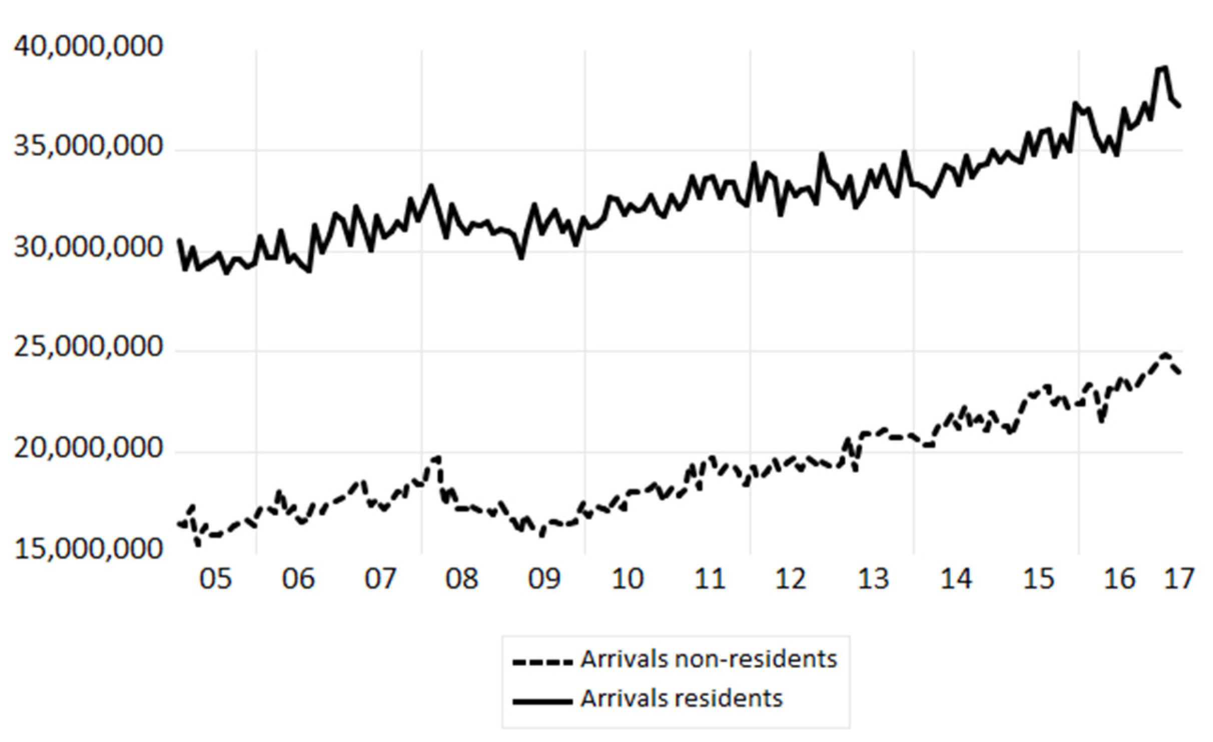
Figure 1.
Arrivals of residents (solid line) and non-residents (dashed line) for the EU-27 (seasonally adjusted by the multiplicative ratio to moving average method). Source: Eurostat and own illustration.
Figure 1.
Arrivals of residents (solid line) and non-residents (dashed line) for the EU-27 (seasonally adjusted by the multiplicative ratio to moving average method). Source: Eurostat and own illustration.

Figure 2.
Overnights of residents (solid line) and non-residents (dashed line) for the EU-27 (seasonally adjusted by the multiplicative ratio to moving average method). Source: Eurostat and illustration.
Figure 2.
Overnights of residents (solid line) and non-residents (dashed line) for the EU-27 (seasonally adjusted by the multiplicative ratio to moving average method). Source: Eurostat and illustration.

Table 1.
Summary ranking of the overall results for arrivals forecasts. Source: European Commission (2017) and own calculations. Boldface indicates the single forecasting model(s)/forecast combination technique(s) characterized by the lowest sum of ranks.
Table 1.
Summary ranking of the overall results for arrivals forecasts. Source: European Commission (2017) and own calculations. Boldface indicates the single forecasting model(s)/forecast combination technique(s) characterized by the lowest sum of ranks.
| Arrivals | 3 Months Non-Residents | 6 Months Non-Residents | 3 Months Residents | 6 Months Residents | Sum | Overall Rank |
|---|---|---|---|---|---|---|
| ARIMA (2,1,0) | 109 | 117 | 119 | 161 | 506 | 4 |
| REGARIMA AR(1) | 194 | 181 | 180 | 144 | 699 | 9 |
| ETS (AIC) | 189 | 199 | 140 | 125 | 653 | 8 |
| ETS (BIC) | 194 | 204 | 168 | 164 | 730 | 10 |
| REGARIMA + Google Trends (EU_trends) | 124 | 72 | 115 | 109 | 420 | 3 |
| REGARIMA + Google Trends (EU_flights) | 132 | 122 | 150 | 158 | 562 | 6 |
| REGARIMA + Google Trends (EU_ hotels) | 117 | 112 | 151 | 152 | 532 | 5 |
| REGARIMA + Google Trends (EU_travel) | 145 | 106 | 154 | 173 | 578 | 7 |
| Combined forecasts (uniform weights) | 59 | 118 | 91 | 76 | 344 | 2 |
| Combined forecasts (Bates–Granger weights) | 57 | 62 | 52 | 54 | 225 | 1 |
Table 2.
Summary ranking of the overall results for overnights forecasts. Source: European Commission (2017) and own calculations. Boldface indicates the single forecasting model(s)/forecast combination technique(s) characterized by the lowest sum of ranks.
Table 2.
Summary ranking of the overall results for overnights forecasts. Source: European Commission (2017) and own calculations. Boldface indicates the single forecasting model(s)/forecast combination technique(s) characterized by the lowest sum of ranks.
| Overnights | 3 Months Non-Residents | 6 Months Non-Residents | 3 Months Residents | 6 Months Residents | Sum | Overall Rank |
|---|---|---|---|---|---|---|
| ARIMA (2,1,0) | 87 | 55 | 138 | 78 | 358 | 3 |
| REGARIMA AR(1) | 132 | 130 | 122 | 103 | 487 | 4 |
| ETS (AIC) | 168 | 211 | 104 | 106 | 589 | 6 |
| ETS (BIC) | 164 | 196 | 117 | 106 | 583 | 5 |
| REGARIMA + Google Trends (EU_trends) | 148 | 127 | 168 | 165 | 608 | 7 |
| REGARIMA + Google Trends (EU_flights) | 173 | 150 | 129 | 154 | 606 | 9 |
| REGARIMA + Google Trends (EU_ hotels) | 171 | 122 | 157 | 168 | 618 | 8 |
| REGARIMA + Google Trends (EU_travel) | 165 | 130 | 165 | 164 | 624 | 10 |
| Combined forecasts (uniform weights) | 63 | 140 | 86 | 101 | 390 | 2 |
| Combined forecasts (Bates–Granger weights) | 49 | 56 | 39 | 59 | 203 | 1 |
© 2020 by the authors. Licensee MDPI, Basel, Switzerland. This article is an open access article distributed under the terms and conditions of the Creative Commons Attribution (CC BY) license (http://creativecommons.org/licenses/by/4.0/).
Share and Cite
MDPI and ACS Style
Gunter, U.; Önder, I.; Smeral, E. Are Combined Tourism Forecasts Better at Minimizing Forecasting Errors? Forecasting 2020, 2, 211-229. https://0-doi-org.brum.beds.ac.uk/10.3390/forecast2030012
AMA Style
Gunter U, Önder I, Smeral E. Are Combined Tourism Forecasts Better at Minimizing Forecasting Errors? Forecasting. 2020; 2(3):211-229. https://0-doi-org.brum.beds.ac.uk/10.3390/forecast2030012
Chicago/Turabian StyleGunter, Ulrich, Irem Önder, and Egon Smeral. 2020. "Are Combined Tourism Forecasts Better at Minimizing Forecasting Errors?" Forecasting 2, no. 3: 211-229. https://0-doi-org.brum.beds.ac.uk/10.3390/forecast2030012