Benchmarking Real-Time Streamflow Forecast Skill in the Himalayan Region

Abstract

Improving decision-making in various areas of water policy and management (e.g., flood and drought preparedness, reservoir operation and hydropower generation) requires skillful streamflow forecasts. Despite the recent advances in hydrometeorological prediction, real-time streamflow forecasting over the Himalayas remains a critical issue and challenge, especially with complex basin physiography, shifting weather patterns and sparse and biased in-situ hydrometeorological monitoring data. In this study, we demonstrate the utility of low-complexity data-driven persistence-based approaches for skillful streamflow forecasting in the Himalayan country Nepal. The selected approaches are: (1) simple persistence, (2) streamflow climatology and (3) anomaly persistence. We generated the streamflow forecasts for 65 stream gauge stations across Nepal for short-to-medium range forecast lead times (1 to 12 days). The selected gauge stations were monitored by the Department of Hydrology and Meteorology (DHM) Nepal, and they represent a wide range of basin size, from ~17 to ~54,100 km². We find that the performance of persistence-based forecasting approaches depends highly upon the lead time, flow threshold, basin size and flow regime. Overall, the persistence-based forecast results demonstrate higher forecast skill in snow-fed rivers over intermittent ones, moderate flows over extreme ones and larger basins over smaller ones. The streamflow forecast skill obtained in this study can serve as a benchmark (reference) for the evaluation of many operational forecasting systems over the Himalayas.

1. Introduction

Skillful streamflow forecasts are critically important in improving decision-making in water-related policy and management (e.g., flood and drought preparedness, reservoir operation and hydropower generation). Real-time streamflow forecasting over the Himalayas remains a critical challenge. (e.g., [1,2]) because of complex basin physiography, shifting weather patterns and sparse distribution of hydrometeorological monitoring stations. The verification of streamflow forecasts can provide insight into hydrologic forecasting by elucidating the level of forecast skill that can be reasonably expected from the forecasting system [3]. In this study, we demonstrate the utility of a persistence-based approach to benchmark forecast skill of the operational streamflow forecasting system in the Himalayan country Nepal.

Nepal is an important part of the Hindu Kush Himalayas (HKH), which are referred to as the water towers of Asia due to the largest concentration of snow and glaciers outside the two poles [4,5,6,7]. The snow cover and glaciers make significant contributions to the hydrology of glacierized basins. Khadka et al. [5] showed, in the simulation study of Tamakoshi basin in eastern Nepal for the years 2000–2009, that snowmelt contributes about 18% of the annual runoff. Further, they showed that the snowmelt represents about 17% of the runoff in the summer season (June to September) while about 25% in the spring season, when the streamflow in these rivers are low. The study by Bhattarai and Regmi [8] in the Langtang river basin in central Nepal shows similar numbers on the contribution of snowmelt to the runoff (~19% on the annual runoff). Dhami et al. [9] used the Soil and Water Assessment Tool and snow-melt runoff model in the Karnali river basin in western Nepal to simulate components of water balance. They reported that about 12% of annual runoff is contributed by the snowmelt, while about 29% by the groundwater base flow.

In Nepal, the Department of Hydrology and Meteorology (DHM) is responsible for monitoring the streamflow at rivers, providing real-time river watch, and developing decision support systems. At present, the real-time river watch system at DHM generates siren alerts at critical stations leveraging the internet and mobile devices for alert delivery [10]. In addition, the community-based early warning system (CBEWS) has been integrated by the early warning system managed by the DHM with the aid of intergovernmental organizations, UN organizations and international non-governmental organizations [11]. CBEWS is inherently people-centric, helping communities use local resources and capacities for flood preparedness efforts [10,11,12]. The simplified data-based mechanistic forecast model was adopted by the DHM to cover the major river basins of Nepal that stem from the mountains to the Terai plains. The integration of the data-based mechanistic model with CBEWS provides an additional lead time of 3–5 h for larger basins and 1–3 h for smaller basins in addition to previous 2–3 h [13]. Owing to the major contribution of snow to the streamflow, particularly in the glacierized basins, persistence-based forecasts could serve as reference to evaluate the skill of the current operational forecasting system, which this study explores. Moreover, this approach could serve as a tool to guide the decision-making pertaining to flood preparedness in the short-medium forecast range.

Hydrologic forecasts are inherently uncertain (e.g., [3,14]). The uncertainty can originate from different sources, including shortcomings in forcing data (e.g., quantitative precipitation forecasts), model structure and parameters, as well as model initial conditions (e.g., [1,14,15,16]). In addition, complex hydrologic processes, such as snowmelt, sub-surface and flow routing, make it more difficult to produce skillful streamflow forecasts in the HKH region (e.g., [1,17]). Most countries in the HKH region are prone to floods (e.g., [1,18]); therefore, achieving skillful forecasts up to the medium range is of utmost importance for flood preparedness efforts. Because of such uncertainties and challenges, achieving skillful streamflow forecasts in this region requires skillful reference forecasting systems. For example, if a reference forecasting system with a low forecast skill is chosen, the operational streamflow (flood) forecasting system might depict higher forecast skill. It will essentially give a false sense of forecast skill associated with the operational system.

The persistence-based approach uses a notion of “tomorrow will be like today” (e.g., [19]). It is tied to the concept of “memory” of any analyzed system [20]: in our case, the basins. One would expect the notion of streamflow persistence to be more pertinent in the glacierized basins due to the relatively slow snowmelt process over time. Though persistence-based forecasts are in use as the reference in the hydrologic forecasting community, their utility across different hydroclimatic conditions and scales have not been fully explored.

Forecasters use various reference forecasts, such as simple persistence, streamflow climatology, a hydrological model fed with zero rainfall and a hydrological model fed with an ensemble of resampled historical rainfall [21], for operational forecast skill verification. Despite some inherent predictability of hydrologic systems due to coupling with the weather and climate system, streamflow shows some likelihood of repetition at seasonal to daily time scales, and hence some inherent predictability [19,20,22]. Den Dool [23] and Fraedrich and Ziehmann-Schlumbohm [24] iterate that only forecasts depicting skill better than persistence can handle the forecast of the time derivative. The degree of persistence, however, might demonstrate variation with location, time of the year and the system studied [23,25]. Den Dool [23] indicated that processes with a long-time scale show higher skill with persistence forecasts, which makes persistence a hard-to-beat method for many complex mechanistic models. Though some authors (e.g., [26]) attribute the streamflow persistence to the carryover storage of water in lakes, and below the land surface, the comprehensive evaluation of persistence-based forecasts was lacking until recently. Palash et al. [1], motivated by the concept of requisite simplicity, showed the utility of a simple linear flood-forecasting system for the Ganges, Brahmaputra and Meghna Rivers, using streamflow persistence as the mechanism of prediction. Recently, Ghimire and Krajewski [19] and Krajewski et al. [27] showed, through a comprehensive study of 140 mid-western agricultural watersheds in the United States, that persistence-based forecast skills show strong dependence with the basin scale, while weaker but non-negligible dependence with the properties of the river network.

In the context of a lack of comprehensive evaluation of persistence-based reference forecasts in the data-scarce Himalayan region, their quantitative assessment can provide the benchmark across scales for any operational forecasting system (e.g., DHM’s forecasting system). This paper specifically explores the following questions: (1) what is the utility of data-driven persistence-based approaches for skillful streamflow forecasting in the Himalayan region? (2) Which forecast conditions, such as lead time, flow threshold, basin size and flow regime (e.g., perennial/snow-fed and intermittent), benefit potential increase in forecast skill? We organize the paper as follows: In Section 2, we discuss the materials and methods used in this study. Section 3 presents results of this study and Section 4 discusses these findings. In Section 5, we summarize and present some conclusions and limitations of this work.

2. Materials and Methods

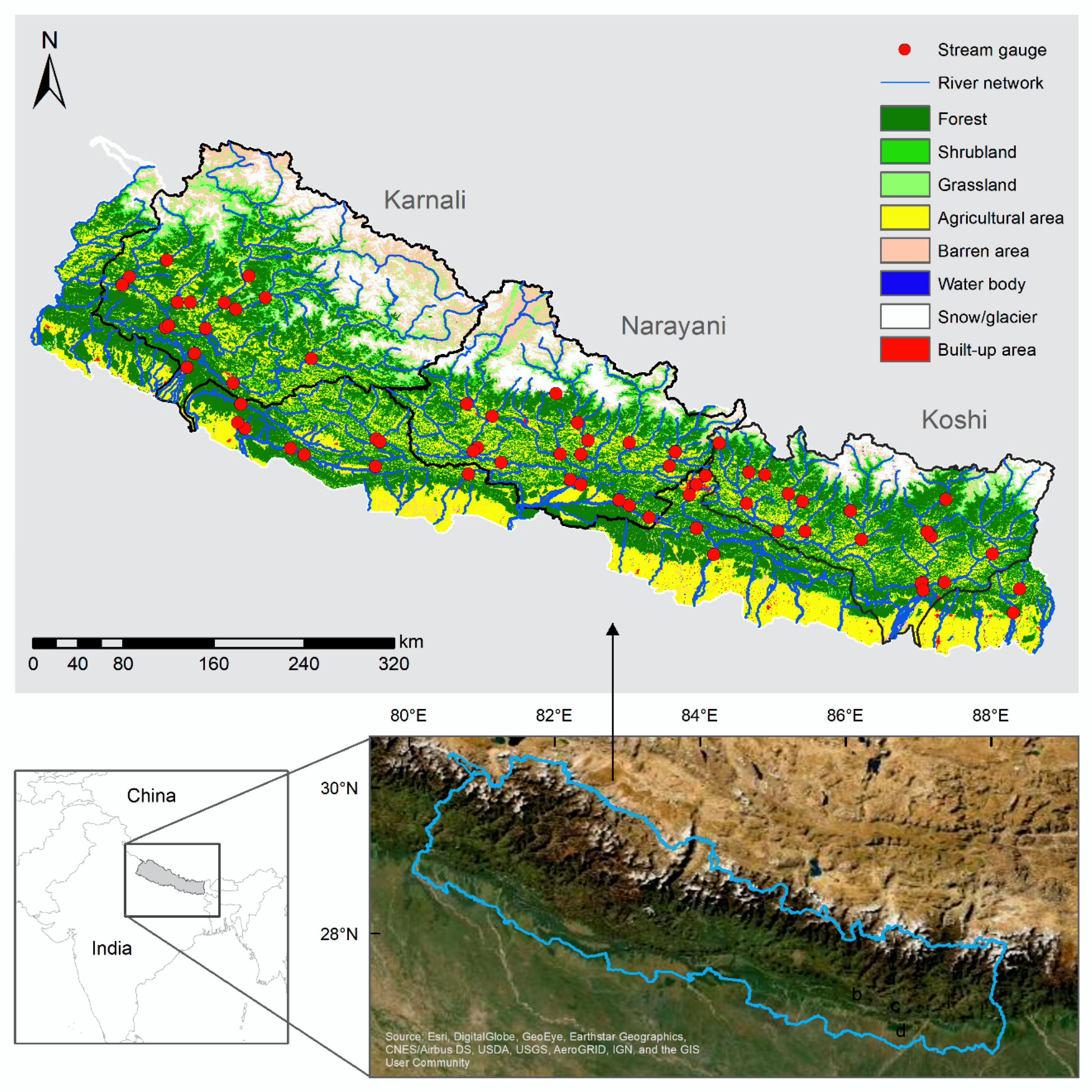
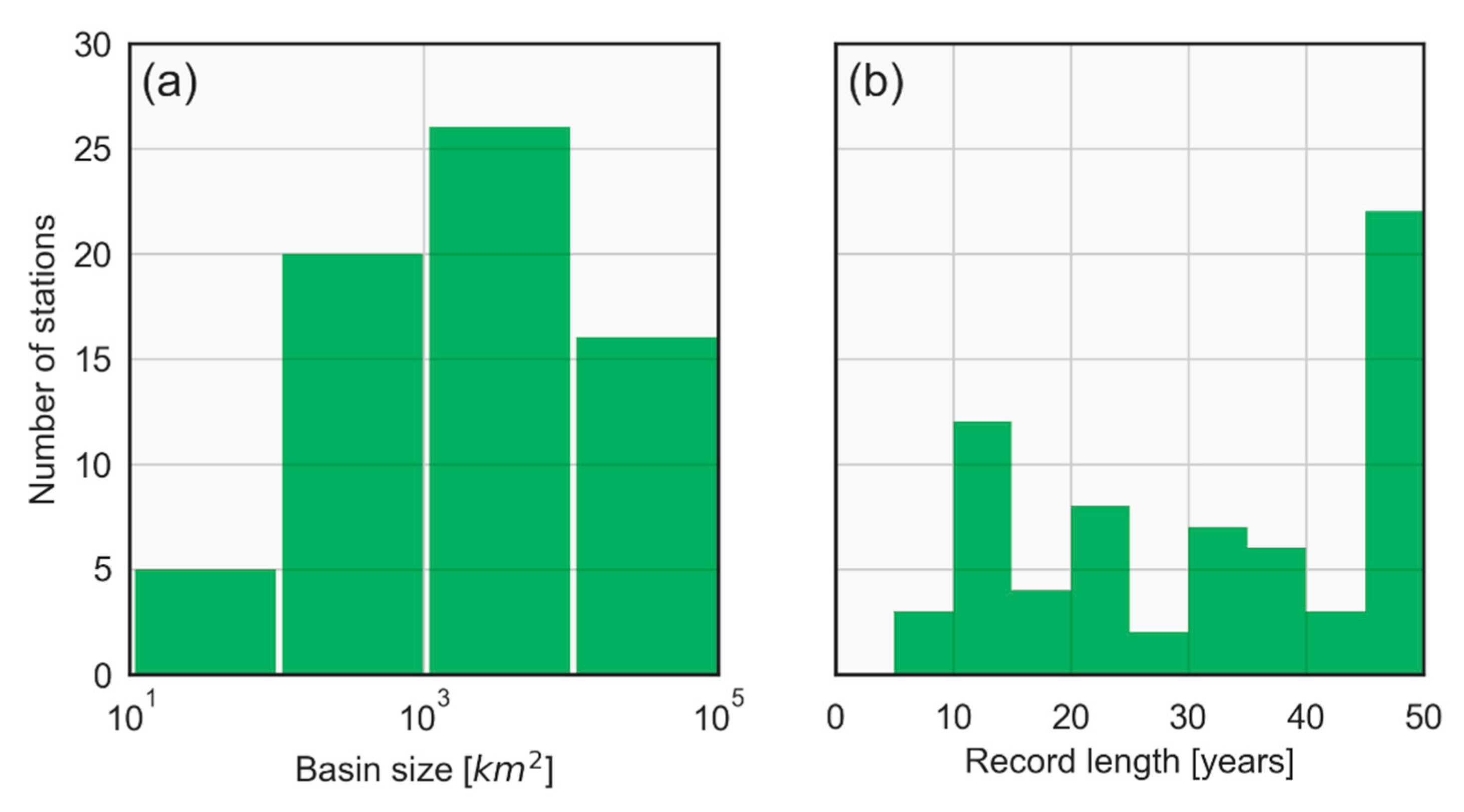
2.1. Study Area and Data

Our domain of interest for this study was Nepal, which is in the central part of Himalayan mountain range. The total area of Nepal is about 147,520 km², located approximately between 80°03′–88°12′ E and 26°21′–30°26′ N (Figure 1). The topographic elevation ranges from 8848m (elevation of Mt. Everest) in the north to 70m in the south above mean sea level featuring diverse climatic conditions varying from polar to tropical [28]. Forest (39.1%), agriculture (29.8%), barren (10.7%) and snow/glaciers (8.2%) are the major land cover types in Nepal [29]. Most of the climate variability in Nepal is attributed to the high reliefs of river catchments e.g., [4]. The climate in Nepal is dominated by a southwestern monsoon (June–September) that originates from the Bay of Bengal and about 80% of precipitation in Nepal occurs only in the monsoon season [30]. The months of October–November occasionally experience post-monsoon rainfall, November–March typically remains dry, and April–May experiences pre-monsoon rainfall [4,5,9,31]. The summer monsoon is more active in the eastern part of Nepal as the monsoon enters and departs from that region, and the winter monsoon is more active in the western region because of the influence of western disturbances [28]. The average annual precipitation (1990–2010) ranges from ~270 mm to ~5500 mm [32]. The consequent runoff during the monsoon accounts for 70%–90% of the annual water balance, as shown in [33].

Most rivers in Nepal drain from north to south and eventually to the Ganges River in India. The rivers in Nepal can be broadly categorized into five major river systems: Karnali, Narayani, Koshi, Mahakali, and the southern and Mahabharat rivers [33]. The former four river systems are combinations of rain- and snow-fed rivers, while the latter river system mostly comprise mid-size rivers, such as the Mechi, Kankai, Kamala, Bagmati, Babai and West Rapti, mostly fed by rainfall and characterized by frequent flash floods [33]. The Karnali, Gandaki and Koshi river systems highlighted in Figure 1 represent about two-thirds of the area of Nepal. These river systems show variability in their hydroclimatic conditions, in addition to the topographic characteristics such as average basin slope and snow cover. In this study, we used historic daily streamflow data at stream gauges stations (red dots in Figure 1) monitored by the DHM across Nepal. Daily streamflow data is the highest-resolution data publicly available from the DHM. It corresponds to the mean values of three readings recorded daily at 8 AM, 12 noon and 4 PM, local time. The streamflow data across stations span between 1962 and 2010, with varying record lengths. Thirty-eight stations have more than 30 years of historical daily streamflow records (Figure A1, Appendix A). We screened the stream gauge stations based on the availability criteria of at least 10 years of streamflow records and at least fair quality data categorized by DHM. The stations that are not shown within the three major river systems correspond to the rivers of the southern and Mahabharat river systems. In total, we used streamflow data from 65 unregulated stream gauge stations. The corresponding basin size varies from ~17 to ~54,100 km², with more than half of the stations monitoring catchments greater than 1000 km² (Figure A1, Appendix A). Note that the hydropower projects built in some of these rivers are run-off-river schemes, which typically do not store the water.

2.2. Experimental Design

Several persistence-based forecast approaches have been discussed in den Dool [19], Wu and Dickinson [23] and Ghimire and Krajewski [25]. Here, we present three of these approaches to generate the reference (benchmark) forecasts in the time domain and evaluate them; these are simple persistence, streamflow climatology and anomaly persistence. Our experimental setup mostly follows the methods outlined in Ghimire and Krajewski [19]. If t represents the time of observation of streamflow Q(t), the forecast for lead time Δt is given by

$$Q\left(t+\Delta t\right)=Q\left(t\right)$$

(1)

Note that the forecasts are generated for the entire streamflow time-series in the records for 65 stream gauge stations in Nepal. While considering the entire time-series, we account for the interannual variability of streamflow.

Here, we use the “climatology” as the average of streamflow on record at time t. The corresponding forecast for lead time Δt is given by

$$Q\left(t+\Delta t\right)=\frac{{{\displaystyle \sum }}_{i=1}^{n}Q\left(t+\Delta t\right)}{n}$$

(2)

where Q(t + Δt) refers to the streamflow at time t + Δt from previous years of record and n refers to the number of years in record.

The anomaly persistence forecast scheme assumes that streamflow anomalies persist over the lead time Δt. The anomalies are computed with respect to the climatology. The anomalies at t and t + Δt i.e., Q′(t) and Q′(t + Δt), respectively, are computed as

$$Q{}^{\prime }\left(t\right)=Q\left(t\right)-clim\left(t\right)$$

(3)

$$Q{}^{\prime }\left(t+\Delta t\right)=Q\left(t+\Delta t\right)-clim\left(t+\Delta t\right)$$

(4)

where clim(t) and clim(t + Δt) are climatology forecasts obtained from Equation (2) at t and t + Δt, respectively. The Equations (3) and (4) yield the forecast at t + Δt as

$$Q\left(t+\Delta t\right)=Q\left(t\right)-clim\left(t\right)+clim\left(t+\Delta t\right)$$

(5)

The forecasts computed in Equations (1)–(5) use the entire streamflow time-series in record, i.e., at least 10 years of streamflow data. Here, we are also interested in exploring the forecast skill associated with the direct runoff component of streamflow. In other words, we computed forecast skill from persistence-based approaches for the rainfall-runoff events. Acknowledging the fact that the separation of runoff components from baseflow is not easy, we used the automated separation technique used by the United States Geological Survey (USGS) called the hydrograph separation program (HYSEP) [34]. The HYSEP employs three methods to separate storm flow from baseflow in the hydrograph: fixed interval, sliding interval, and local minimum. The duration of the surface runoff is computed empirically by

$$K=A^{0.2}$$

(6)

where K is the number of days after which the surface runoff stops and A is the upstream drainage area of the basin in sq. miles [34]. The interval used to separate the storm flow is 2K*, which should be the nearest odd integer to 2K. The hydrograph separation starts one interval, i.e., 2K* days, before the start of the date selected for the start of the separation, while it ends 2K* days after the selected date. For further details of the separation technique, refer to Sloto and Crouse [34]. Figure A2 of the Appendix A shows the demonstration of storm flow separation across two river basins (small and large scales) using the sliding interval method.

2.3. Evaluation Metrics

We used several standard hydrologic forecast evaluation measures to evaluate the forecasts described in Section 2.2. The metrics we computed were Kling–Gupta efficiency (KGE), mean absolute error (MAE), normalized MAE (nMAE), timing of the hydrographs (T_H) and peak difference (PD). The KGE comprises three components: Pearson’s correlation coefficient (r), variance ratio (α) and mean ratio (β) (refer to [35]). It is given by

$$KGE=1-\sqrt{{\left(r-1\right)}^2+{\left(\alpha -1\right)}^2+{\left(\beta -1\right)}^2}$$

(7)

where $\alpha =\frac{{\sigma }_f}{{\sigma }_o} and \beta =\frac{{\mu }_f}{{\mu }_o}$. σ_f and σ_o correspond to the standard deviations of forecasts and observed streamflow, respectively. μ_f and μ_o correspond to the means of forecasts and observed streamflow, respectively. The ideal value of KGE is equal to 1, which can be obtained when all three components attain values of 1. For example, if the values of α and β are close to 1, the corresponding KGE is dominated by the correlation component. By construction, the KGE associated with the persistence-based forecasts is dominated by correlation. When the mean of the observations is used as a benchmark, the frontier of the KGE separating between the good model and the bad model is equal to −0.41 see [36]. In our discussion, we primarily focus on the KGE.

We compute the MAE associated with the forecasts as below:

$$MAE=\frac{{\displaystyle \sum }\left|Q_f-Q_o\right|}{N}$$

(8)

where Q_f is the streamflow forecast, Q_o is the observation and N is the number of data pairs. For fair comparison across the basin scales, we normalize MAE by the upstream drainage area to compute nMAE. The hydrograph timing (T_H) is computed as the number of hours a hydrograph requires to be shifted so that the cross-correlation between the forecasts and the observations is maximized. By construction, T_H is close to the lead time of the forecast. The peak difference (PD) in percentage is computed as

$$PD=\frac{pea{k}_f-pea{k}_o}{N}\times 100$$

(9)

where peak_f and peak_o are peaks of the forecast and the observations, respectively.

3. Results

In this section, we present key results from our experiment evaluating persistence-based reference forecasts at 65 stream gauge stations in the Himalayan region in Nepal. First, we present results for three major river systems (basin-wise forecasts), and then for the entire region (regional forecasts).

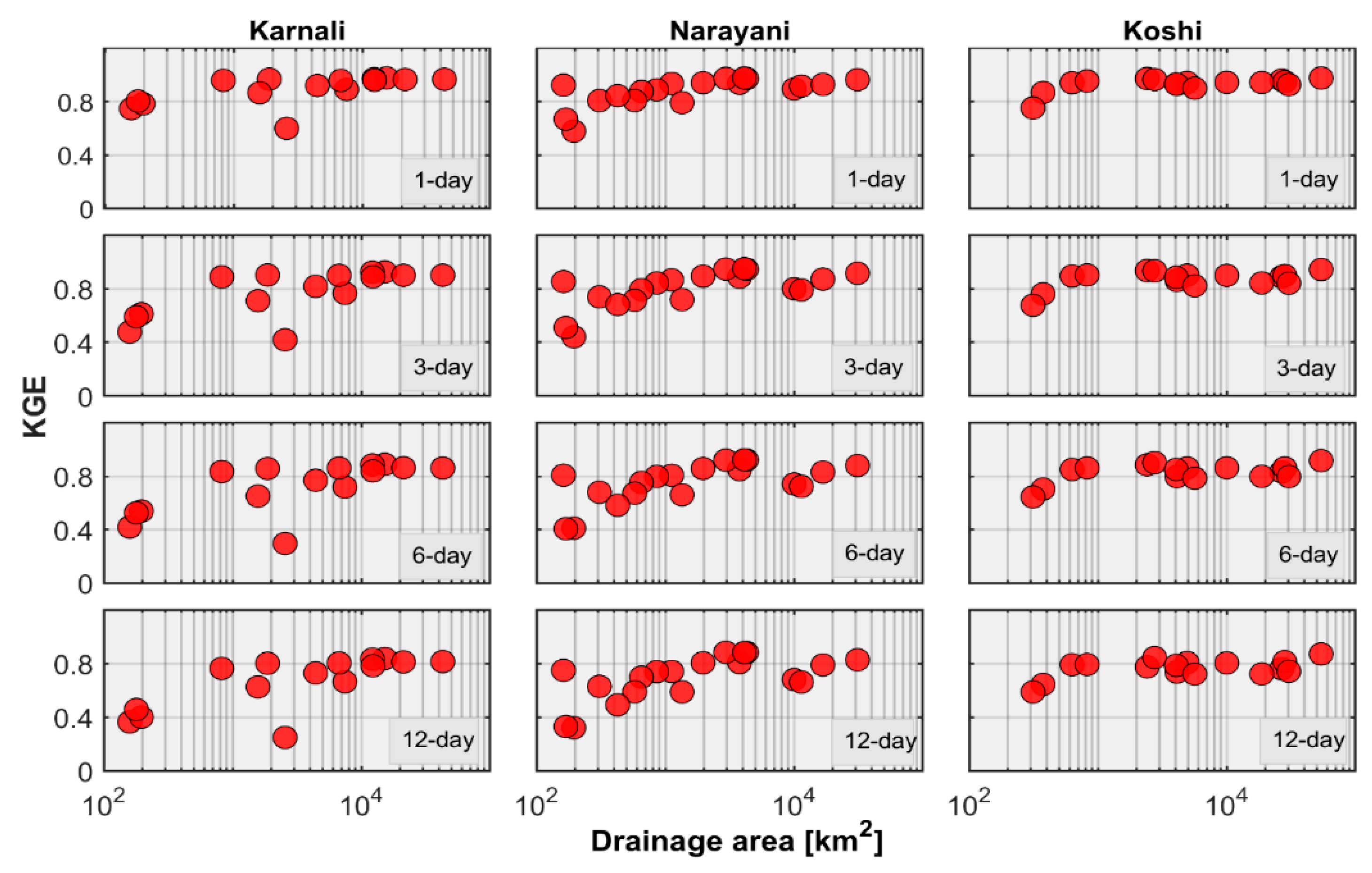
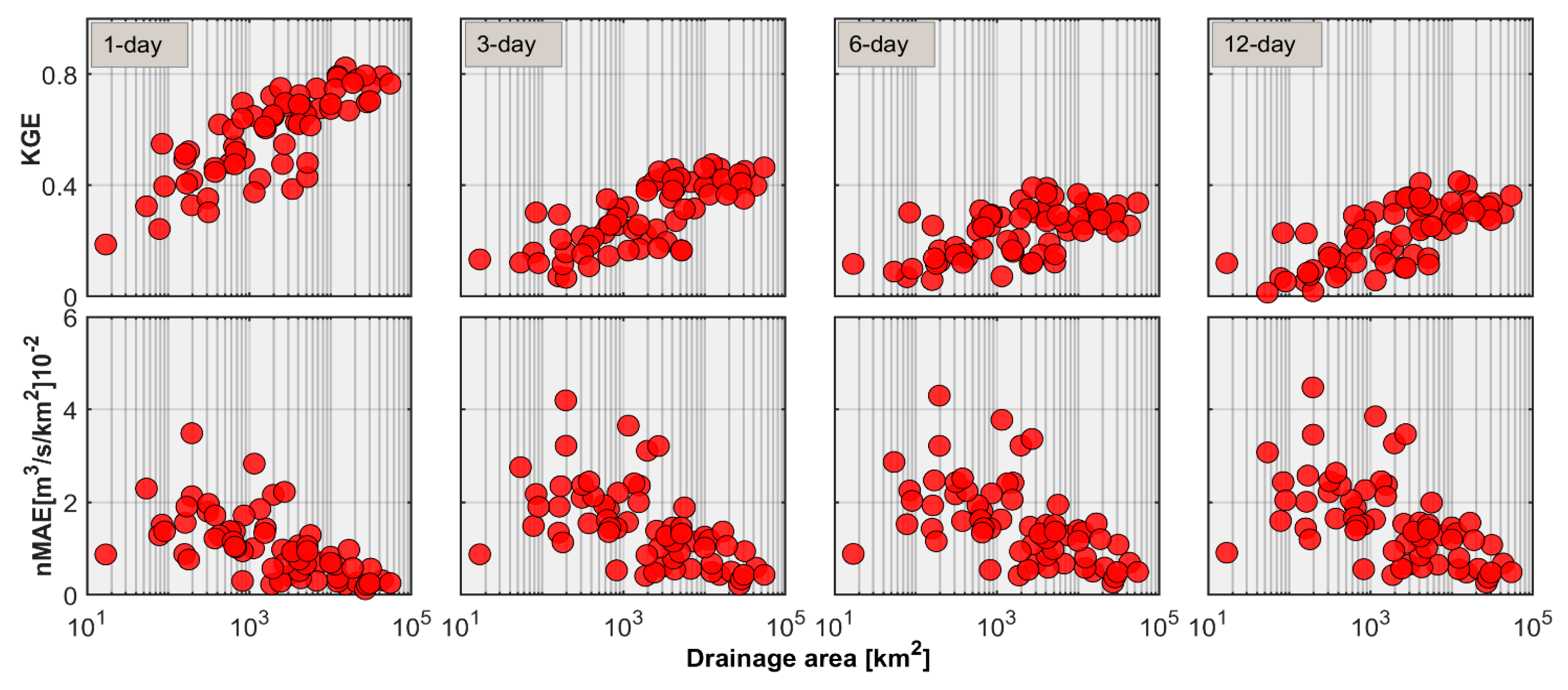
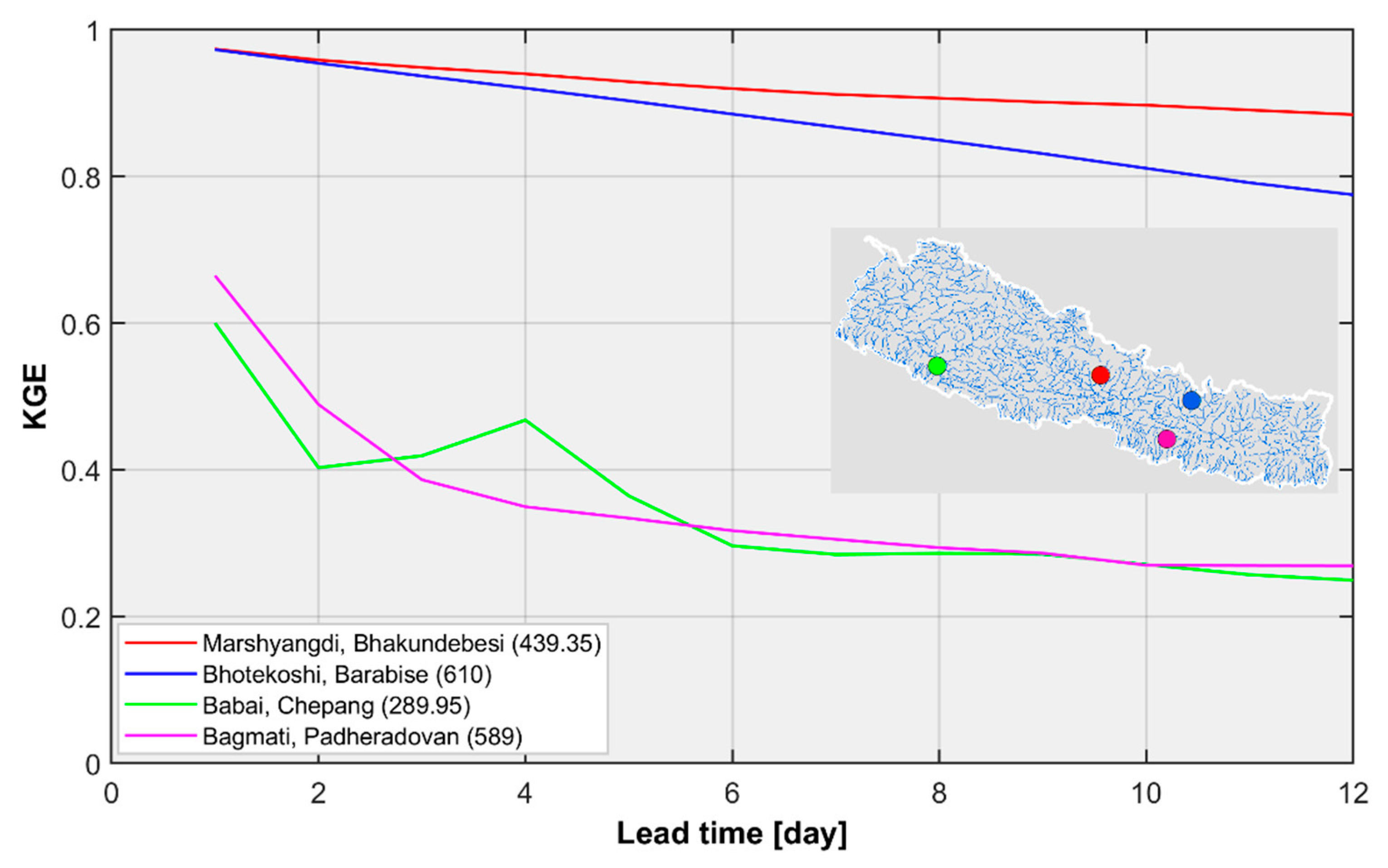
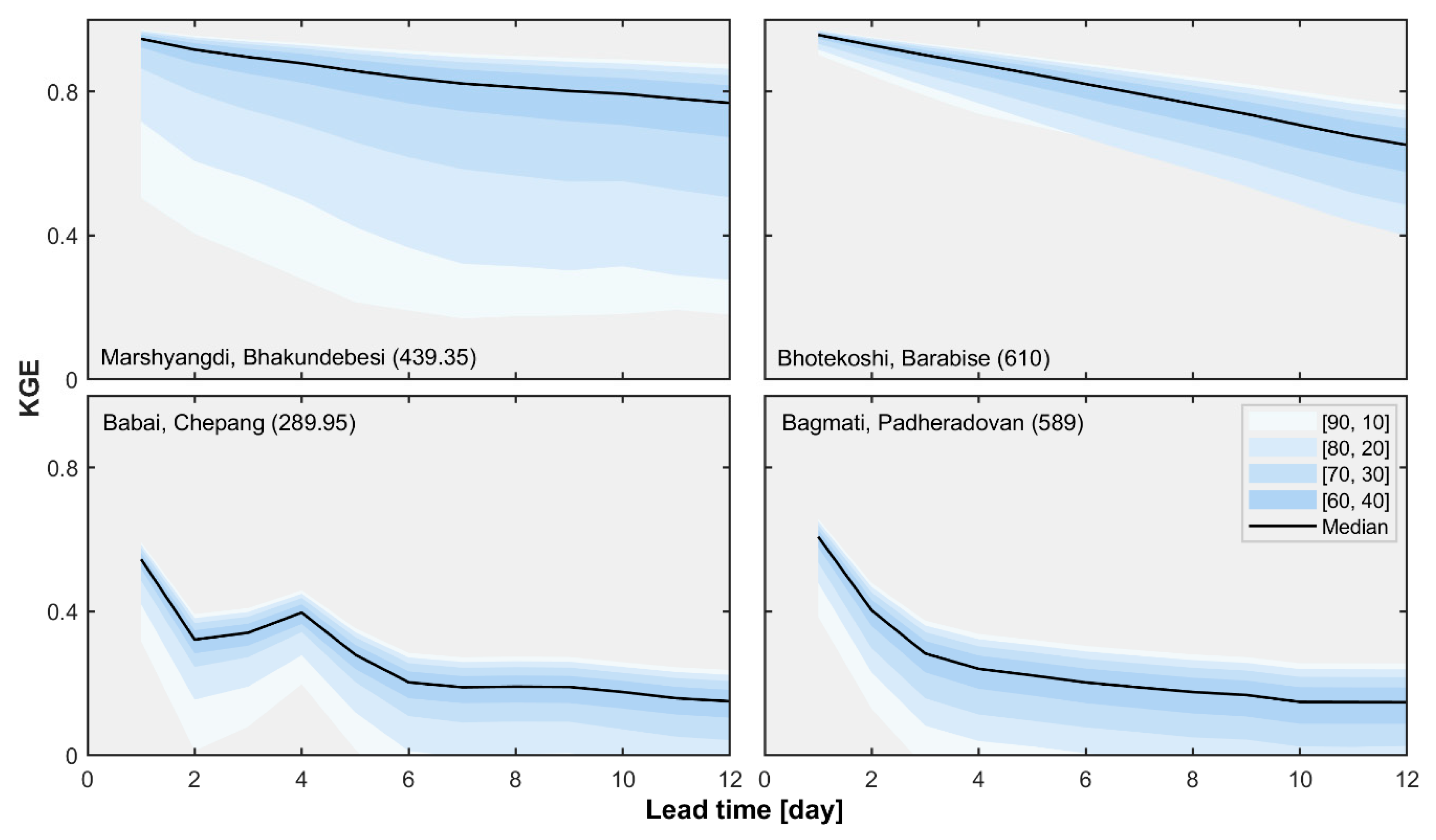
3.1. Basin-Wise Forecasts

Our notion behind exploring basin-wise forecast skill is due to the variability of snow/glacier cover, storage conditions and hydroclimatic conditions across three major river basins. In Figure 2, we show the variability of the KGE metric with drainage area for three major river systems of Nepal (Karnali, Narayani and Koshi) across forecast lead times of 1, 3, 6 and 12-days. The result corresponds to the simple persistence forecasts. For simple persistence forecasts, the KGE is dominated by the correlation component r. For all three basins across most of the stations, KGE > 0.8 for the lead time of 1-day. The stronger relationship between the KGE and basin size emerges with the increasing forecast lead times. Note that the pattern is not as strong in the Koshi river basin, but the KGE values are relatively higher across basin scales. In addition, there are not many smaller monitored basins in the Koshi river system to exactly decide on the pattern relative to other two river systems. The overall results across three river systems clearly show a strong spatio-temporal dependence of simple persistence-based forecast skill.

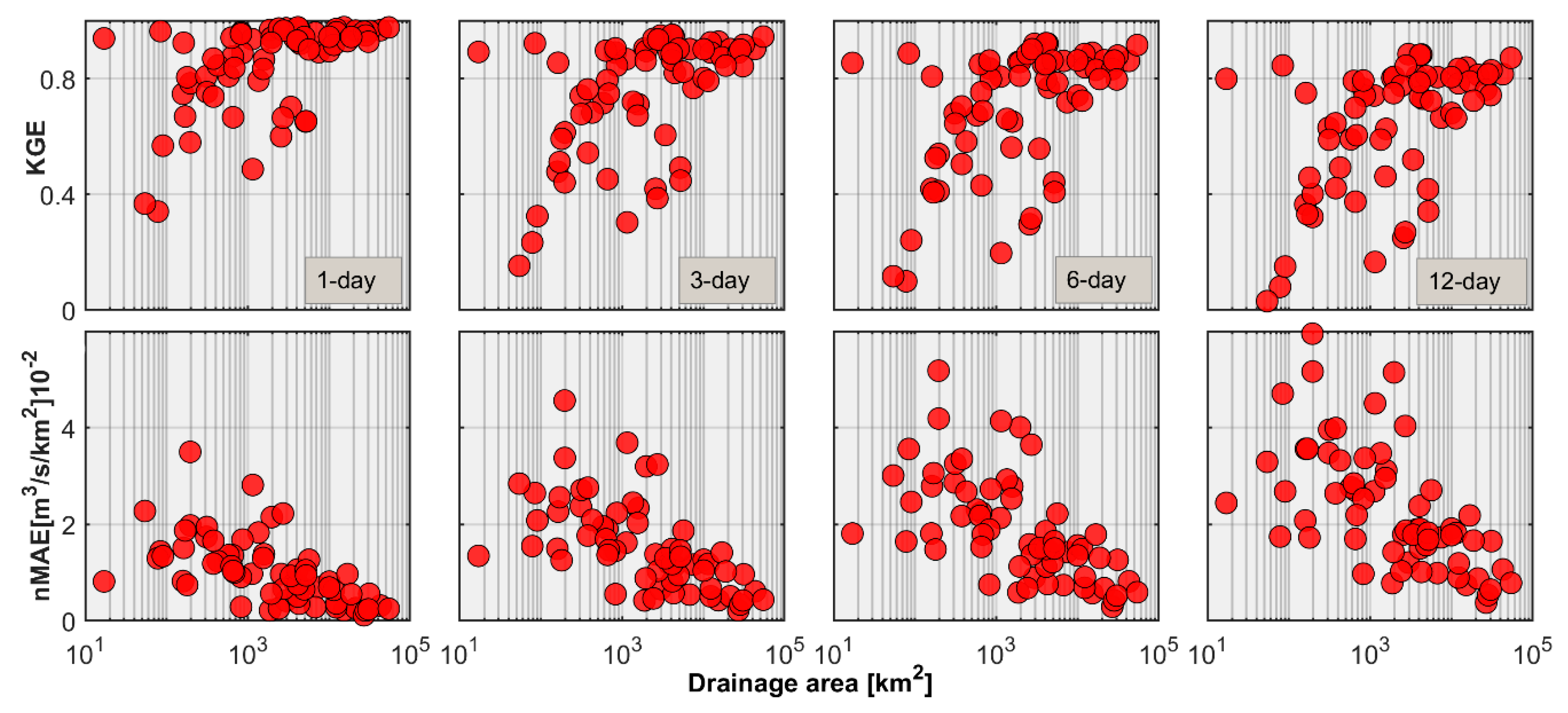
3.2. Regional Streamflow Forecasts

The results from basin-wise forecasts show that no distinct pattern of forecast skill emerges across major river systems in Nepal. Therefore, we decided to pool all stations from three major river systems, including the mid-sized river stations from other river basins (see Figure 1), and refer to their forecasts as regional forecasts. In Figure 3, we present results in terms of two skill metrics, i.e., KGE (first row) and nMAE (second row), based on simple persistence forecasts (Equation (1)). The relationship between the KGE and basin size is more prominent for pooled stations across lead times of the forecast. There are, however, few stations which diverge from the overall pattern of the KGE observed in the basin-wise forecast evaluation. We explore the forecast performance associated with these stations separately (see Figure A3, Appendix A). We find that their forecast skills show more variability and decay much faster with forecast lead times. In addition, these stations are mostly mid-sized river basins associated with the intermittent flow regime. We present the detailed discussion on the origin of their forecast skill later. Note that basins > 1000 km² show relatively higher forecast skill (KGE~0.7) even at the lead time of 12 days. The values of nMAE also depict similar dependence with basin size as the KGE. The values of nMAE show a much stronger relationship with basin scale at shorter lead times, while starting to diverge at longer lead times particularly for small basin scales of size < 1000 km². By construction, PD for the simple persistence forecast is close to 0. In addition, by construction, PD for the climatology-based forecasts does not vary with lead times (see Figure A4, Appendix A). The corresponding median value of PD across basins in Nepal is about −76% (underestimation of the peak). For anomaly persistence, however, the median values of PD across basins range from about −1.5% to −3% at lead times of 1 day to 12 days, respectively (see Figure A4, Appendix A). Note that climatology-based forecasts show sizable a dependence of PD on basin size, while this is not apparent for anomaly persistence-based forecasts.

In this section, we evaluate the forecast performance associated with various reference forecast schemes described in Section 2. Here, we present the one-to-one comparison of forecast skill in terms of KGE (first row) and nMAE (second row) between these schemes in Figure 4. Apparently, persistence-based forecasts outperform climatology-based forecasts at shorter lead times across all basin scales. Both simple persistence and climatology-based forecasts perform similarly for longer lead times. Anomaly persistence, however, performs similarly with simple persistence for shorter lead times, while it outperforms simple persistence for longer lead times at smaller basin scales (also see Figure 5). Note that climatology is an integral component of anomaly persistence forecasts. Therefore, the improved skill of anomaly persistence at longer lead times and smaller basin scales could be attributed to the improved performance of climatology-based forecasts at longer lead times.

From the real-time streamflow forecasting point of view, it would be more informative to explore how KGE evolves over time across basin scales. In Figure 5, we show that the evolution of KGE skill is associated with three methods across four nested basins in the Karnali river system (refer inset). In addition to the apparent strong dependence of KGE with basin scales, the temporal evolutive pattern of KGE shows variability across basin scales. For example, the smallest basin (A~159 km²) depicts the sharp drop in the KGE metric up to lead time of four days and remains stable from thereon. However, as the basin size increases, the rate of decrease of the KGE metric becomes slower. The other important observation is that up to about four days of lead time, both persistence-based forecast schemes outperform climatology-based forecasts. After four days of lead time, the difference between climatology and anomaly persistence-based forecast skill is negligible. Note, however, that the difference in KGE between simple persistence and other two forecast schemes shows systematic decrease with the increasing basin scales.

The results presented above are associated with the entire streamflow time-series. In other words, the forecast skills computed originate from the contribution of both baseflow and stormflow. However, the intrinsic question is whether we can achieve similar forecast performance for the storm flow (i.e., direct runoff component of hydrographs). In Figure 6, we present the forecast performance based on simple persistence for the direct runoff obtained using HYSEP described in Section 2. As we demonstrate through stormflow hydrographs in Figure A5, Appendix A, at a lead time of one day, the simple persistence-based forecasts are essentially delayed by one day. In other words, the timing of forecast hydrographs and the timing of the extreme event peak are delayed by one day, while preserving the magnitude of the peak of the hydrograph. Note the damping of smaller rainfall-runoff event stormflows in the smaller nested basin (see a, Figure A5, Appendix A) by the river network aggregation process at the larger basin (see b, Figure A5, Appendix A). The resulting pattern of both KGE and nMAE with basin scales is similar to the one presented before. Notably, reasonable KGE could be achieved for a one-day-ahead stormflow forecast, while showing significant decline for longer lead times. Note that the basins of size > 1000 km² still show KGE > 0.3 for 12 days ahead forecast, illustrating the potential of using it as reference forecast for the evaluation of stormflow forecasts particularly at short-range.

As we highlighted in Section 2, our region predominantly contains rivers in the perennial flow regime (snow/glacier fed). There are, however, some rivers originating in the southern plains of Nepal which are predominantly in the intermittent flow regime. Since we established the fact that forecast skill shows strong spatial scale dependence, it would be of interest to the forecasting community to explore the dependence on the flow regimes. The ideal comparison would be to evaluate forecasts conditional on the basin scale. We identified four basins of a size of ~2500 km²; two perennial river basins in northern Nepal and the other two intermittent river basins in southern Nepal (see inset of Figure 7). Figure 7 demonstrates the evolution of KGE (simple persistence-based) with lead times for these four basins. A distinct pattern of KGE evolution emerges. The perennial rivers depict higher forecast performance with gradual decline in the forecast performance with forecast horizon (lead time) while the intermittent rivers show sharp decline in the forecast performance with forecast horizon. Since intermittent rivers are mostly driven by rainfall-runoff events, their forecast skill evolution shows similar behavior elucidated by the results in Figure 6. Note a sudden spike of KGE for the Babai river at four days of lead time. Though it is hard to point out explicitly the reason, one could attribute it to the ability of four days ahead forecast to capture two consecutive historic floods (separated by 4 days) in the year 2015.

It is extremely important for forecasters to achieve good predictability of higher flow quantiles for flood preparedness and mitigation efforts. For the same four basins, we evaluate the forecast performance associated with the different streamflow quantiles. We refer to flow quantiles as flow threshold. Figure 8 shows the evolution of KGE across lead times for various flow quantiles. KGE reported here is computed for the streamflow forecasts exceeding the corresponding flow quantile. Note that as the flow quantile increases, the sample size used to compute the forecast skill systematically decreases. Given that we evaluate the forecast skill using the continuous streamflow time-series in record, we consider the sample size to be enough for the evaluation. Clearly, the KGE for the intermittent rivers (lower panel) shows sharp decline for the higher flow quantiles. The perennial rivers (upper panel), however, depict much better forecast performance even for the higher flow quantiles at longer lead times. However, of the two, the Marshyangdi basin at Bhakundebesi, shows relatively faster decline in the performance of flows exceeding 60th percentile. As Ghimire and Krajewski [19] highlighted, this variability in KGE could be explained by the difference in their river network geometries, typically explained by the network width function see [37,38] for detail. Explicit attribution is beyond the scope of this paper.

4. Discussion

A clear signature emerging out of our persistence-based streamflow forecasts skill is its strong spatio-temporal dependence. Our results substantiate it further. The results from Figure 3 and Figure 6 demonstrate that significant contribution to the persistence-based forecast skill is from the baseflow contribution. In other words, the contribution from snowpack (snow/glacier), groundwater and storage in the contributing catchments plays an important role in the streamflow hydrographs, particularly for the perennial rivers in the Himalayan region of Nepal. Typically, the streamflow predictability at small basin scales is more tied to the rainfall than the large basin scales. We highlighted this fact through our results for the intermittent rivers. The perennial rivers, however, receive sizable contributions from the base flow relative to the rainfall even in the small basin scales, hence the relatively good forecast skill. Moreover, the persistence-based forecast derives skill from the memory of the system, in this case river catchments. The larger the basin scales, the longer the memory of the catchments, and hence the long-range persistence. We show from our results that higher forecast skill (KGE > 0.7) could be achieved for a basin size larger than 1000 km², even at a longer forecast horizon. Another important contribution to the skillful forecasts of larger basins at longer lead times is from the water transport in the river network, where the streamflow aggregation process controls the shape of the streamflow fluctuations [27,39,40,41]. In addition to the land surface (e.g., catchment) memory, the streamflow predictability has a strong connection to the persistence in the land surface initial hydrologic conditions (e.g., soil moisture, groundwater, current streamflow and snowpack) [42,43,44], providing the main source for the skillful streamflow forecasts.

The dependence of forecast skill depicted in this study with the basin size and forecast lead times is consistent with the results presented in Ghimire and Krajewski [19]. Given a large number of glacierized basins in the region, as opposed to agricultural watersheds used in the study of Ghimire and Krajewski [19], more stations depict higher streamflow forecast skill. For instance, at a lead time of one day, we show a median value of KGE of about 0.92 in the region, compared to the median value of KGE of about 0.78 presented in their study. Therefore, our results demonstrate a clear implication of persistence-based forecasts for the real-time streamflow forecasting in the Himalayan region. Our illustration of reasonably good streamflow forecast skill across spatial and temporal scales provides a reliable benchmark (reference) to evaluate the efficacy of the operational real-time streamflow forecasting. Particularly for the larger basin scales, we are able to show that it is difficult for many operational mechanistic hydrologic models to outperform persistence-based forecast skills. Any operational forecasting scheme that can aptly depict forecast skill better than the three-reference forecast schemes presented in this study, can be considered skillful. We are able to show quantitatively that it can serve as a skillful reference for the evaluation of real-time flood forecasts (higher flow quantiles) up to the medium range for perennial rivers while up to the short-range for the intermittent rivers. Our findings clearly show that persistence-based forecast scheme, anomaly persistence in particular, could provide skillful reference forecasts for the evaluation of current operational streamflow forecasting systems in the Himalayan country of Nepal. Moreover, it could provide guidance to the flood related decision-making process, especially in the short-medium forecast range.

5. Conclusions

In this study, we explored the utility of persistence-based forecasting schemes to benchmark the real-time streamflow forecasting system in the Himalayan region of Nepal. We used the daily streamflow data at 65 stream gauge stations monitored by the DHM, Nepal, to generate the forecasts and evaluate the associated skills in the short-to-medium forecast horizon. To this end, we employed three reference forecast schemes: (i) simple persistence, (ii) streamflow climatology and (iii) anomaly persistence. Based on the results from this study, we could reach at following conclusions:

▪

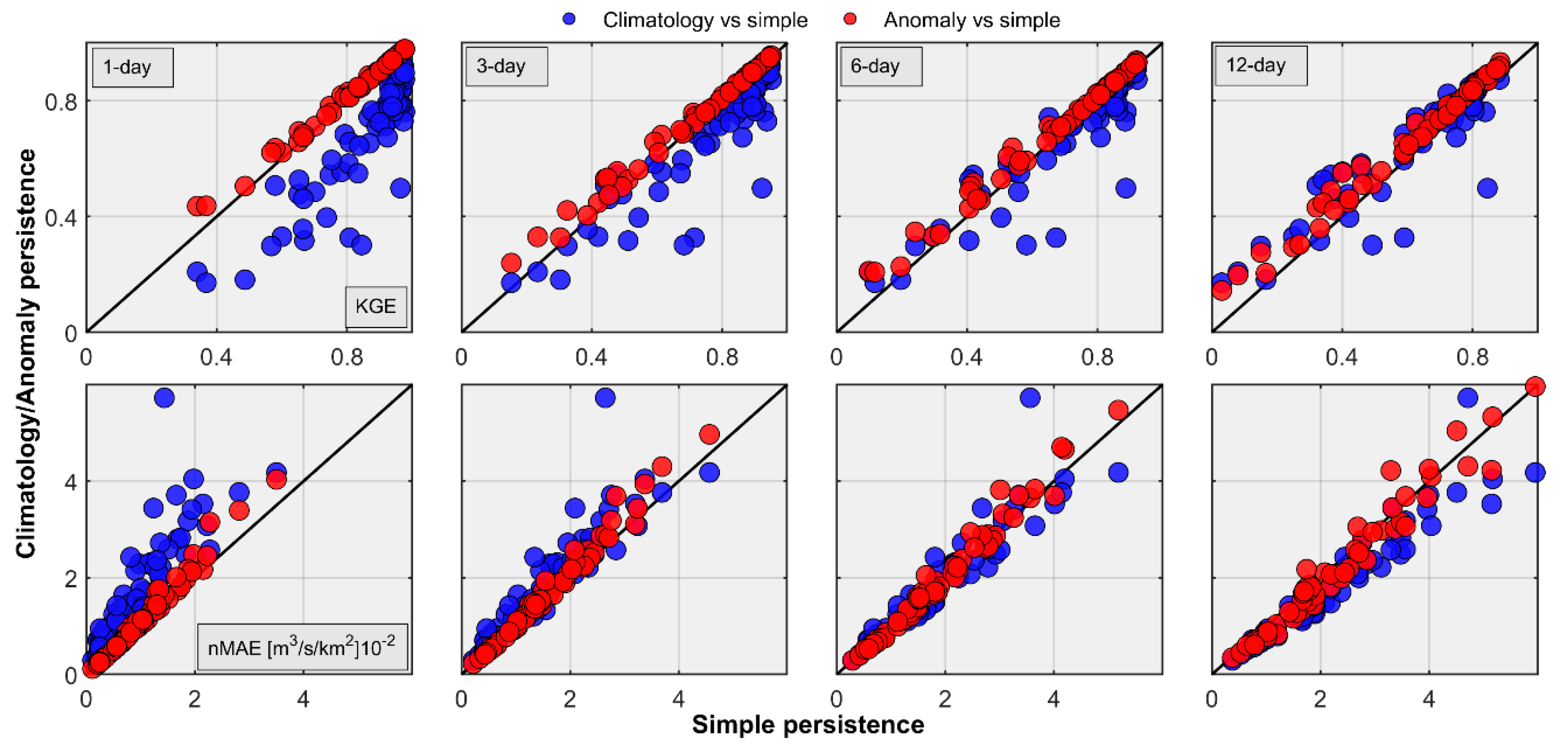
Persistence-based forecast skill shows strong dependence with the basin scale and forecast lead time. Anomaly persistence forecasts outperform others at small basin scales and longer lead times and hence can be a better selection for benchmarking the real-time streamflow forecasting system in the Himalayan region of Nepal.

▪

The forecast skill shows strong dependence with the flow regime and flow threshold. The verification results show higher forecast skill for perennial rivers over intermittent rivers and moderate flow quantiles over high flow quantiles.

This study highlights the fact that a persistence-based forecast scheme is difficult to outperform using many mechanistic hydrologic models, particularly for larger basin scales in the Himalayan region. The findings from this study have implications for evaluating real-time streamflow forecasts from the operational forecasting system across basin scales and lead times in this region. Moreover, it provides insights on designing the streamflow monitoring network for future applications.

Our study, however, is not without limitations. We did not account for the measurement uncertainty associated with streamflow observations. We considered the published streamflow data to be within the acceptable limit of observational uncertainty. We did not account for the uncertainty associated with the rating curves. Moreover, we could not perform the sub-daily forecast skill evaluation due to the unavailability of published sub-daily streamflow observations. We expect that the analysis using sub-daily streamflow data will not lead to a significantly different inference regarding the forecasting performance of persistence-based systems, which we could explore further in our future research.

References

1. Palash, W.; Jiang, Y.; Akanda, A.S.; Small, D.L.; Nozari, A.; Islam, S. A Streamflow and Water Level Forecasting Model for the Ganges, Brahmaputra, and Meghna Rivers with Requisite Simplicity. J. Hydrometeorol. 2018, 19, 201–225. [Google Scholar] [CrossRef]
2. Pellicciotti, F.; Buergi, C.; Immerzeel, W.W.; Konz, M.; Shrestha, A.B. Challenges and Uncertainties in Hydrological Modeling of Remote Hindu Kush-Karakoram-Himalayan (HKH) Basins: Suggestions for Calibration Strategies. Mt. Res. Dev. 2012, 32, 39–50. [Google Scholar] [CrossRef]
3. Sharma, S.; Siddique, R.; Reed, S.; Ahnert, P.; Mendoza, P.; Mejia, A. Relative effects of statistical preprocessing and postprocessing on a regional hydrological ensemble prediction system. Hydrol. Earth Syst. Sci. 2018, 22, 1831–1849. [Google Scholar] [CrossRef] [Green Version]
4. Gurung, D.R.; Giriraj, A.; Aung, K.S.; Shrestha, B.; Kulkarni, A.V. Snow-Cover Mapping and Monitoring in the Hindu Kush-Himalayas; The International Centre for Integrated Mountain Development: Lalitpur, Nepal, 2011; pp. 1–44. [Google Scholar]
5. Khadka, D.; Babel, M.S.; Shrestha, S.; Tripathi, N.K. Climate change impact on glacier and snow melt and runoff in Tamakoshi basin in the Hindu Kush Himalayan (HKH) region. J. Hydrol. 2014, 511, 49–60. [Google Scholar] [CrossRef]
6. Paudel, K.P.; Andersen, P. Monitoring snow cover variability in an agropastoral area in the Trans Himalayan region of Nepal using MODIS data with improved cloud removal methodology. Remote Sens. Environ. 2011, 115, 1234–1246. [Google Scholar] [CrossRef]
7. Mukherji, A.; Molden, D.; Nepal, S.; Rasul, G.; Wagnon, P. Himalayan waters at the crossroads: Issues and challenges. Int. J. Water Resour. Dev. 2015, 31, 151–160. [Google Scholar] [CrossRef] [Green Version]
8. Bhattarai, B.C.; Regmi, D. Impact of Climate Change on Water Resources in View of Contribution of Runoff Components in Stream Flow: A Case Study from Langtang Basin, Nepal. J. Hydrol. Meteorol. 2016, 9, 74–84. [Google Scholar] [CrossRef] [Green Version]
9. Dhami, B.; Himanshu, S.K.; Pandey, A.; Gautam, A.K. Evaluation of the SWAT model for water balance study of a mountainous snowfed river basin of Nepal. Environ. Earth Sci. 2018, 77, 1–20. [Google Scholar] [CrossRef]
10. Government of Nepal Ministry of Energy Water Resources and Irrigation; Department of Hydrology and Meteorology. Standard Operating Procedure for Flood Early Warning System in Nepal; Department of Hydrology and Meteorology: Kathmandu, Nepal, 2018.
11. Gautam, D.K.; Phaiju, A.G. Community Based Approach to Flood Early Warning in West Rapti River Basin of Nepal. J. Integr. Disaster Risk Manag. 2013, 3, 155–169. [Google Scholar] [CrossRef]
12. Smith, P.J.; Brown, S.; Dugar, S. Community-based early warning systems for flood risk mitigation in Nepal. Nat. Hazards Earth Syst. Sci. 2017, 17, 423–437. [Google Scholar] [CrossRef] [Green Version]
13. Budimir, M.; Donovan, A.; Brown, S.; Shakya, P.; Gautam, D.; Uprety, M.; Cranston, M.; Sneddon, A.; Smith, P.; Dugar, S. Communicating Complex Forecasts for Enhanced Early Warning in Nepal. Geosci. Commun. Discuss. 2019, 1–32. [Google Scholar] [CrossRef] [Green Version]
14. Liu, Y.; Gupta, H.V. Uncertainty in hydrologic modeling: Toward an integrated data assimilation framework. Water Resour. Res. 2007, 43, 1–18. [Google Scholar] [CrossRef]
15. Sharma, S.; Siddique, R.; Balderas, N.; Fuentes, J.D.; Reed, S.; Ahnert, P.; Shedd, R.; Astifan, B.; Cabrera, R.; Laing, A.; et al. Eastern U.S. verification of ensemble precipitation forecasts. Weather Forecast. 2017, 32, 117–139. [Google Scholar] [CrossRef]
16. Pappenberger, F.; Scipal, K.; Buizza, R. Hydrological aspects of meteorological verification. Atmos. Sci. Lett. 2008, 9, 43–52. [Google Scholar] [CrossRef]
17. Kayastha, R.B.; Steiner, N.; Kayastha, R.; Mishra, S.K.; Forster, R.R. Comparative Study of Hydrology and Icemelt in Three Nepal River Basins Using the Glacio-Hydrological Degree-Day Model ( GDM ) and Observations From the Advanced Scatterometer. Front. Earth Sci. 2020, 7, 1–13. [Google Scholar] [CrossRef] [Green Version]
18. WRI Aqueduct Global Flood Risk Country Rankings. 2015. Available online: https://www.wri.org/resources/data-sets/aqueduct-global-flood-risk-country-rankings (accessed on 29 June 2020).
19. Ghimire, G.R.; Krajewski, W.F. Exploring Persistence in Streamflow Forecasting. J. Am. Water Resour. Assoc. 2020, 56, 542–550. [Google Scholar] [CrossRef]
20. Mittermaier, M.P. The Potential Impact of Using Persistence as a Reference Forecast on Perceived Forecast Skill. Weather Forecast. 2008, 23, 1022–1031. [Google Scholar] [CrossRef]
21. Bennett, J.C.; Robertson, D.E.; Shrestha, D.L.; Wang, Q.J. Selecting reference streamflow forecasts to demonstrate the performance of NWP-forced streamflow forecasts. In Proceedings of the 20th International Congress on Modelling and Simulation, Adelaide, Australia, 1–6 December 2013; pp. 2611–2617. [Google Scholar]
22. Ghimire, G.R.; Jadidoleslam, N.; Krajewski, W.F.; Tsonis, A.A. Insights On Streamflow Predictability Across Scales Using Horizontal Visibility Graph Based Networks. Front. Water 2020. accepted for publication. [Google Scholar]
23. van den Dool, H. Empirical Methods in Short-Term Climate Prediction; Oxford University Press: Oxford, UK, 2007; ISBN 0-19-920278-8/978-0-19-920278-2. [Google Scholar]
24. Fraedrich, K.; Ziehmann-Schlumbohm, C. Predictability Experiments with Persistence Forecasts in a Red-noise Atmosphere; Royal Meteorological Society: Reading, UK, 1994; ISBN 0035-9009. [Google Scholar]
25. Wu, W.; Dickinson, R.E. Warm-season rainfall variability over the U.S. Great Plains and its correlation with evapotranspiration in a climate simulation. Geophys. Res. Lett. 2005, 32, 215. [Google Scholar] [CrossRef]
26. Pagano, T.; Garen, D. A Recent Increase in Western U.S. Streamflow Variability and Persistence. J. Hydrometeorol. 2005, 6, 173–179. [Google Scholar] [CrossRef] [Green Version]
27. Krajewski, W.F.; Ghimire, G.R.; Quintero, F. Streamflow Forecasting without Models. J. Hydrometeorol. 2020, in press. [Google Scholar]
28. Karki, R.; Talchabhadel, R.; Aalto, J.; Baidya, S.K. New climatic classification of Nepal. Theor. Appl. Climatol. 2016, 125, 799–808. [Google Scholar] [CrossRef]
29. Uddin, K.; Shrestha, H.L.; Murthy, M.S.R.; Bajracharya, B.; Shrestha, B.; Gilani, H.; Pradhan, S.; Dangol, B. Development of 2010 national land cover database for the Nepal. J. Environ. Manag. 2015, 148, 82–90. [Google Scholar] [CrossRef]
30. Shrestha, M.L. Interannual variation of summer monsoon rainfall over Nepal and its relation to Southern Oscillation Index. Meteorol. Atmos. Phys. 2000, 75, 21–28. [Google Scholar] [CrossRef]
31. Mool, P.K.; Wangda, D.; Bajracharya, S.R.; Joshi, S.P.; Kunzang, K.; Gurung, D.R. Inventory of Glaciers, Glacial Lakes and Glacial Lake Outburst Floods: Monitoring and Early Warning Systems in the Hindu Kush-Himalayan Region—Bhutan; International Centre for Integrated Mountain Development: Khumaltar, Nepal, 2001. [Google Scholar]
32. DHM, N. Climate Normals; The Department of Hydrology and Meteorology: Kathmandu, Nepal, 2010.
33. Gautam, M.R.; Acharya, K. Streamflow trends in Nepal. Hydrol. Sci. J. 2012, 57, 344–357. [Google Scholar] [CrossRef]
34. Sloto, R.a.; Crouse, M.Y. Hysep: A Computer Program for Streamflow Hydrograph Separation and Analysis; Water-Resources Investigations Report 96-4040; U.S. Geological Survey: Reston, VA, USA, 1996; p. 54.
35. Gupta, H.V.; Kling, H.; Yilmaz, K.K.; Martinez, G.F. Decomposition of the mean squared error and NSE performance criteria: Implications for improving hydrological modelling. J. Hydrol. 2009, 377, 80–91. [Google Scholar] [CrossRef] [Green Version]
36. Knoben, W.J.M.; Freer, J.E.; Woods, R.A. Technical note: Inherent benchmark or not? Comparing Nash-Sutcliffe and Kling-Gupta efficiency scores. Hydrol. Earth Syst. Sci. Discuss. 2019, 23, 4323–4331. [Google Scholar] [CrossRef] [Green Version]
37. Rodriguez-Iturbe, I.; Rinaldo, A. Fractal River Basins: Chance and Self-Organization; Cambridge University Press: Kolkata, India, 1997; ISBN 0521004055. [Google Scholar]
38. Perez, G.; Mantilla, R.; Krajewski, W.F. The influence of spatial variability of width functions on regional peak flow regressions. Water Resour. Res. 2018, 54, 7651–7669. [Google Scholar] [CrossRef]
39. Ayalew, T.B.; Krajewski, W.F.; Mantilla, R. Connecting the power-law scaling structure of peak-discharges to spatially variable rainfall and catchment physical properties. Adv. Water Resour. 2014, 71, 32–43. [Google Scholar] [CrossRef]
40. Ayalew, T.B.; Krajewski, W.F.; Mantilla, R.; Small, S.J. Exploring the effects of hillslope-channel link dynamics and excess rainfall properties on the scaling structure of peak-discharge. Adv. Water Resour. 2014, 64, 9–20. [Google Scholar] [CrossRef]
41. Ayalew, T.B.; Krajewski, W.F.; Mantilla, R. Analyzing the effects of excess rainfall properties on the scaling structure of peak discharges: Insights from a mesoscale river basin. Water Resour. Res. 2015, 51, 3900–3921. [Google Scholar] [CrossRef]
42. Arnal, L.; Wood, A.W.; Stephens, E.; Cloke, H.L.; Pappenberger, F. An efficient approach for estimating streamflow forecast skill elasticity. J. Hydrometeorol. 2017, 18, 1715–1729. [Google Scholar] [CrossRef]
43. Harrigan, S.; Prudhomme, C.; Parry, S.; Smith, K.; Tanguy, M. Benchmarking ensemble streamflow prediction skill in the UK. Hydrol. Earth Syst. Sci. 2018, 22, 2023–2039. [Google Scholar] [CrossRef] [Green Version]
44. Wood, A.W.; Pagano, T.; Roos, M. Tracing The Origins of ESP, HEPEX Blog. 2016. Available online: https://hepex.inrae.fr/tracing-the-origins-of-esp/ (accessed on 29 June 2020).
Figure 1. Location of the study domain, Nepal. The white patches in the terrain map (not to scale) depict the snow cover (Nepal Himalaya). The land cover is from Uddin et al. [29]. The red dots represent stream gauge stations monitored by the Department of Hydrology and Meteorology (DHM), Nepal.
Forecasting 02 00013 g001
Figure 2. Relationship between the Kling–Gupta Efficiency (KGE) and drainage area across three major basins in Nepal. The columns show the Karnali, Narayani and Koshi river basins while the rows show lead times of 1, 3, 6 and 12 days, respectively.
Forecasting 02 00013 g002
Figure 3. Relationship of skill metrics with drainage area for the entire Nepal. The columns show 1, 3, 6 and 12 day lead times, while the rows show Kling–Gupta efficiency (KGE) and normalized mean absolute error (nMAE), respectively.
Forecasting 02 00013 g003
Figure 4. One-to-one relationship of skill metrics between climatology and simple persistence-based forecasts (blue), and between anomaly persistence-based forecasts and simple persistence-based forecasts (red). The columns show 1, 3, 6 and 12 day lead times, while the rows show Kling–Gupta efficiency (KGE) and normalized mean absolute error (nMAE), respectively.
Forecasting 02 00013 g004
Figure 5. Evolution of KGE metric with lead time across increasing basin scales (ad) shown in the inset. The panels show the KGE comparison between three methods: simple persistence, anomaly persistence and climatology.
Forecasting 02 00013 g005
Figure 6. Relationship of skill metrics with drainage area for event-based streamflow. The columns show 1, 3, 6 and 12 day lead times, while the rows show Kling–Gupta efficiency (KGE) and normalized mean absolute error (nMAE), respectively.
Forecasting 02 00013 g006
Figure 7. Evolution of Kling-Gupta efficiency (KGE) metric with lead time. The lines in the top (red and blue) represent snow-fed river basins while the lines in the bottom (green and magenta) represent intermittent river basins. Note that all four river basins are of a similar size of ~2500 km2.
Forecasting 02 00013 g007
Figure 8. Percentile plots showing the evolution of Kling–Gupta efficiency (KGE) with lead time for four river basins described in Figure 7. Each percentile refers to the KGE computed for streamflow forecasts exceeding corresponding percentile flow. For example, 90th percentile KGE represents the KGE computed for streamflow forecasts >90th percentile flow. The envelope corresponds to each 10th quantile on either side of the median flow. The higher and lower flow quantiles shown in the interval correspond to the lower and upper bounds of the envelope, respectively. For example, the interval [90, 10] corresponds to the KGE computed for 90th and 10th percentile flows, respectively.
Forecasting 02 00013 g008