
A Stochastic Estimation Framework for Yearly Evolution of Worldwide Electricity Consumption


Department of Data Science & Artificial Intelligence, Faculty of Information Technology, University of Petra, Amman 1196, Jordan
Forecasting 2021, 3(2), 256-266; https://0-doi-org.brum.beds.ac.uk/10.3390/forecast3020016
Submission received: 7 February 2021
/
Revised: 24 March 2021
/
Accepted: 29 March 2021
/
Published: 1 April 2021
(This article belongs to the Section Power and Energy Forecasting)
Abstract
:The determination of electric energy consumption is remarked as one of the most vital objectives for electrical engineers as it is highly essential in determining the actual energy demand made on the existing electricity supply. Therefore, it is important to find out about the increasing trend in electric energy demands and use all over the world. In this work, we present a prediction scheme for the progression of worldwide aggregates of cumulative electricity consumption using the time series of the records released annually for the net electricity use throughout the world. Consequently, we make use of an autoregressive (AR) model by retaining the best possible autoregression order recording the highest regression accuracy and the lowest standardized regression error. The resultant regression scheme was proficiently employed to regress and forecast the evolution of next-decade data for the net consumption of electricity worldwide from 1980 to 2019 (in billion kilowatt-hours). The experimental outcomes exhibited that the highest accuracy in regressing and forecasting the global consumption of electricity is 95.7%. The prediction results disclose a linearly growing trend in the amount of electricity issued annually over the past four decades’ observation for the global net electricity consumption dataset.
1. Introduction
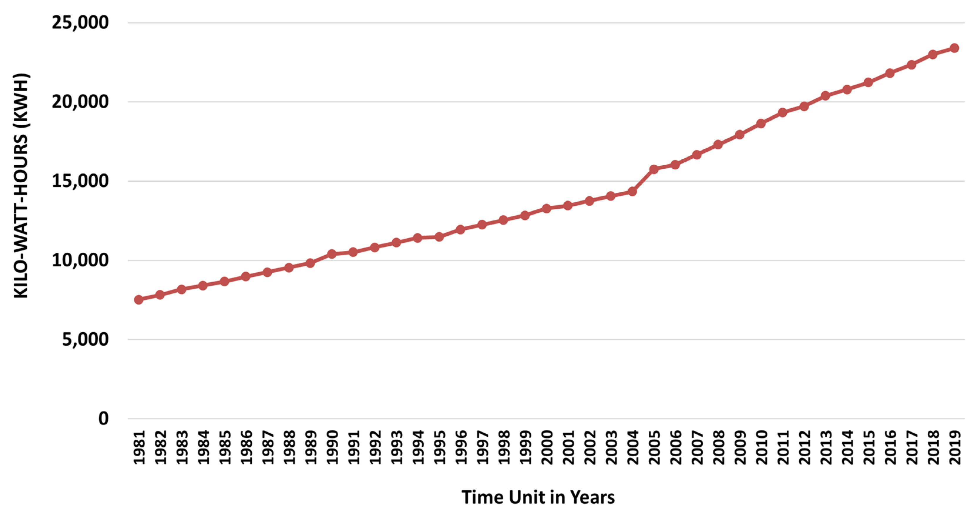
Electricity consumption is an imperative commercial indicator and holds a substantial responsibility in developing the energy advancement strategy for every country [1]. Worldwide electric energy consumption grew from 7323 TWh in 1980 to 23.4 TWh in 2019 [2]. Normally, countries with greater populations consume extra electric power. For instance, China and the United States are among the highest per capita consumers of electricity in the world, consuming 4.55 and 12.6 MWh, respectively, in 2017 [3]. However, Canada is one of the highest consumers of electricity at 14.3 MWh per capita, despite having a population of about 36 million residents. Per capita consumption of electricity can vary widely due to electricity rates, appliance penetration, market saturation, and heating and cooling. However, the accumulated amounts of global electric energy consumption have been observed and collected in time-based data items over the past four decades. To illustrate the data distribution of the given time series, Figure 1 shows the actual dataset of the annual releases of worldwide past statistics of the worldwide cumulative electric energy consumption releases between 1980 and 2019 [4,5]. In 2019, the world’s electricity consumption amounted to approximately 23.4 trillion kWh. One quadrillion watts is approximately equal to one petawatt. Indeed, in 2019, the worldwide consumption of electrical energy increased at a markedly slower rate than the previous years as a result of the slowdown in economic progression and more moderate temperatures in several large countries [5].
Certainly, the determination of the electricity consumption trend is observed as one of the most essential targets in electrical power engineering as it is highly essential for environmental engineering and information technology [6]. Consequently, it is essential to find out about the increasing tendency of the statistics of worldwide electric energy consumption. Generally speaking, a time-series technique can be used to analyze the deposition rate of electricity consumption. However, an extraordinarily powerful autoregressive signal technique can be used as a modeling and processing technique to predict the trend. The parametric regression processes have been largely employed as multidisciplinary tools for time-series regression, interpolation, and extrapolation. Examples of employing the parametric regression model in time-series regression and estimation can be found in [7,8,9,10,11,12,13,14,15]. Therefore, the work of this paper employs the parametric regression method to develop an estimation scheme for the aforementioned annual reports of electricity consumption rates based on the data collected from the previous time sequences with optimal forecasting accuracy.
Recently, several signal prediction techniques, including multivariate analysis methods and artificial intelligence techniques [16,17,18,19,20,21], have been commonly suggested to cope with the dependence of electricity consumption projection on a large number of chronological records and training samples to attain accurate projections [22,23]. Moreover, some related statistical methodologies require the records to match specific statistical assumptions like following a normal distribution [24]. Hence, to build a forecasting scheme for electricity consumption, a prediction process is required to perform well using a small number of past records that may not meet any statistical assumptions [25,26]. In this research, we make use of the autoregression system (AR process) to redevelop and then examine the dataset of the yearly launch for net electric energy consumption of the preceding four decades (1980–2019) by exploiting the best possible regression accuracy with the lowest possible accumulative regression error. Particularly, the key contributions of this work can be summarized as follows:
- We develop an autoregression process scheme that preserves an optimal degree of regression and prediction accuracy with minimum modeling error for the collected electricity data records.
- We analyze the experimental findings of the original dataset in conjunction with the forecasted datasets to demonstrate the importance and efficiency of the established scheme.
The remainder of this paper is organized as follows: Section 2 defines the regression scheme using autoregression method. Section 3 depicts and analyzes the experimental findings by contemplating a number of situations. Finally, Section 4 provides the inferences and remarks for the proposed work and findings.
2. Autoregressive AR(p) Process Modeling
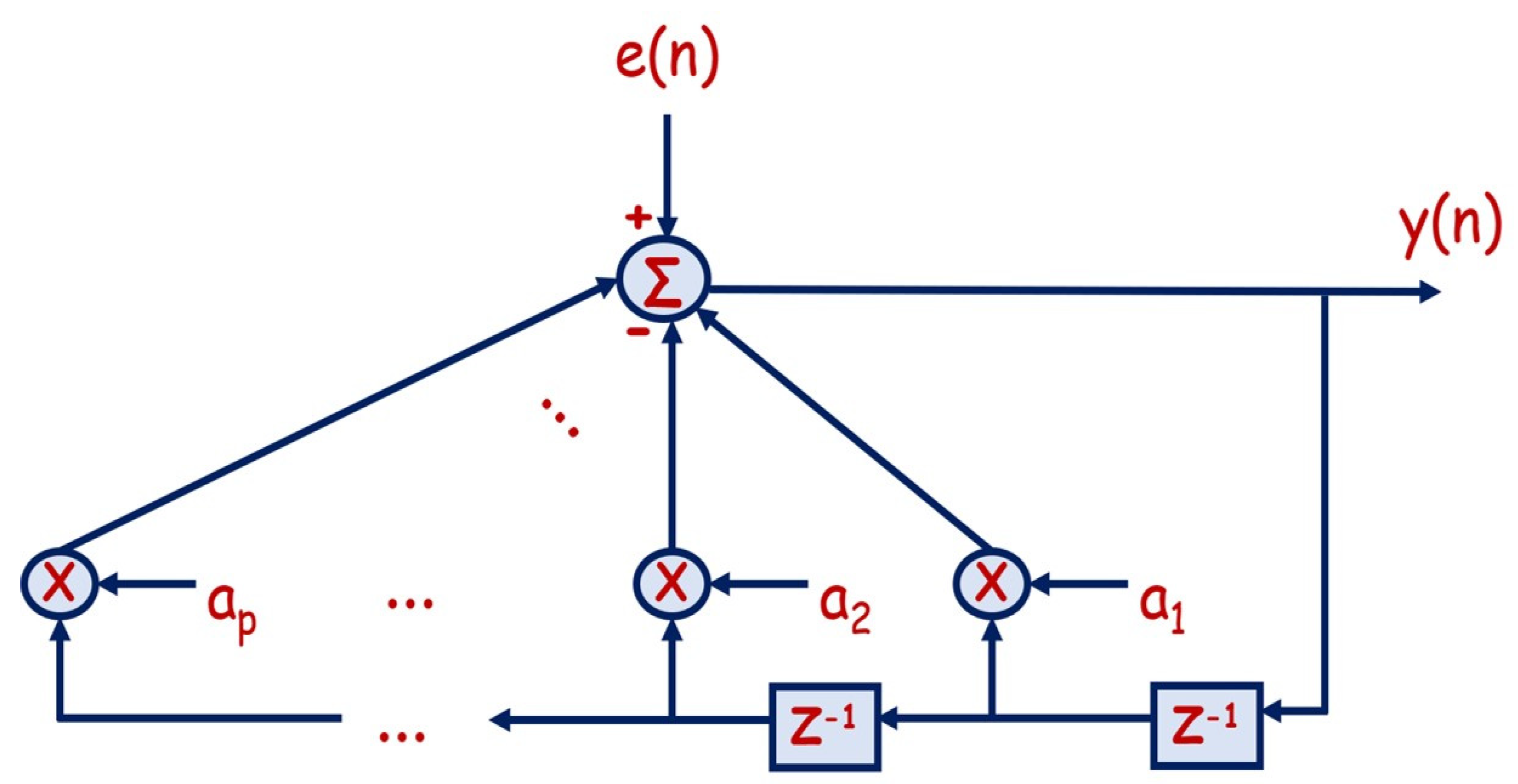
The autoregressive (AR) model is a parametric approach for signal (i.e., time-series/ data points) spectrum modeling and estimation [27]. It can be used to grant a linear framework to approximate the signal dynamics over time and predict (forecast) the momentary future behavior based totally on previous conduct of the time series. This could be accomplished by means of employing the time-series regression and estimation strategies on the current time-sequence statistics against one or more previous values in the equal series. In ), the value p is known as the model order for the autoregressive process. For example, an would be a “first-order autoregressive process” in which the outcome variable of technique at some factor in time t is related only to time durations at t-1 solely (i.e., the value of the variable at one period apart). For the second-order process, the consequence variable of technique at time t is associated solely with periods at t-1 and t-2 (i.e., the value of the variable at two durations apart) and so on. The widespread structure of the AR model can be realized as illustrated in Figure 2.
According to Figure 2, the mathematical expression of the AR process can be derived for any order as follows:
- The first-order AR process is obtained with one parameter according to the following formula:
- The second-order AR process is obtained with two parameters according to the following formula:
- The pth order AR process is obtained with parameters according to the following formula:where y(n) is the original dataset, is the estimated dataset, and e(n) is the accumulative autoregression error. Actually, to maintain the best autoregression process for dataset interpolation and extrapolation/estimation, the optimum autoregression order needs to be reached, which can be attained only when the accumulative autoregression/perdition error is minimized. Consequently, solving the computational minimization problem for the accumulative autoregression error can lead to computing the parameters for the autoregression process using autocorrelation function (ACF) Ryy(k) as follows:
For better understanding, let us consider the third-order AR process (), which is obtained with three parameters according to the following formula:
To develop this third-order model, one needs to find the parameters a1, a2, and a3. Therefore, we need to expand j to 1, 2, and 3 and apply them as follows:
Then, we come up with a system of equations with three unknowns: a1, a2, a3. Such an algebraic system can be solved using several numerical methods such as using the matrix system known as the Toeplitz matrix [28]. The obtained system can subsequently be applied for both time-series regression and estimation.
Nonetheless, the appropriate order for the autoregression process varies amongst the time-series records since it principally depends on the diversity of interpretations through the time-series records in addition to the extent of linearity along with the data records of the time-series itself [29]. Figure 3 illustrates the block diagram for the autoregression modeling methodology steps from scattered data points to the regularized predicted data points. As shown in the illustration, the data points are supplied into the parametric scheme for the interpolation process using the highest relevant regression order and therefore commissioned to foresee/extrapolate the forthcoming developments of the interpolated dataset [29].
3. Electricity Consumption Estimation Schemes
Autoregression process is a recursive parameter-oriented method for time-series/dataset regression and estimation. The basic idea of such a parametric scheme is that process is obtained by a means of a stochastic difference equation via developing the regression process parameters that fulfill the ultimate modeling order for each dataset record. Definitely, the process with the smallest error value and suitable design cost is the primary model (i.e., it is preferable to choose the model with the lowest regression order that maximizes the regression confidence while minimizing the complexity of the system). In order to accomplish this, one should investigate and analyze the relationship between the various regression process orders with respect to their subsequent accumulative regression error values. In this work, we have developed an autoregression system using MATLAB to reproduce the time-series data-records for the yearly publication of the aforementioned electricity consumption dataset.
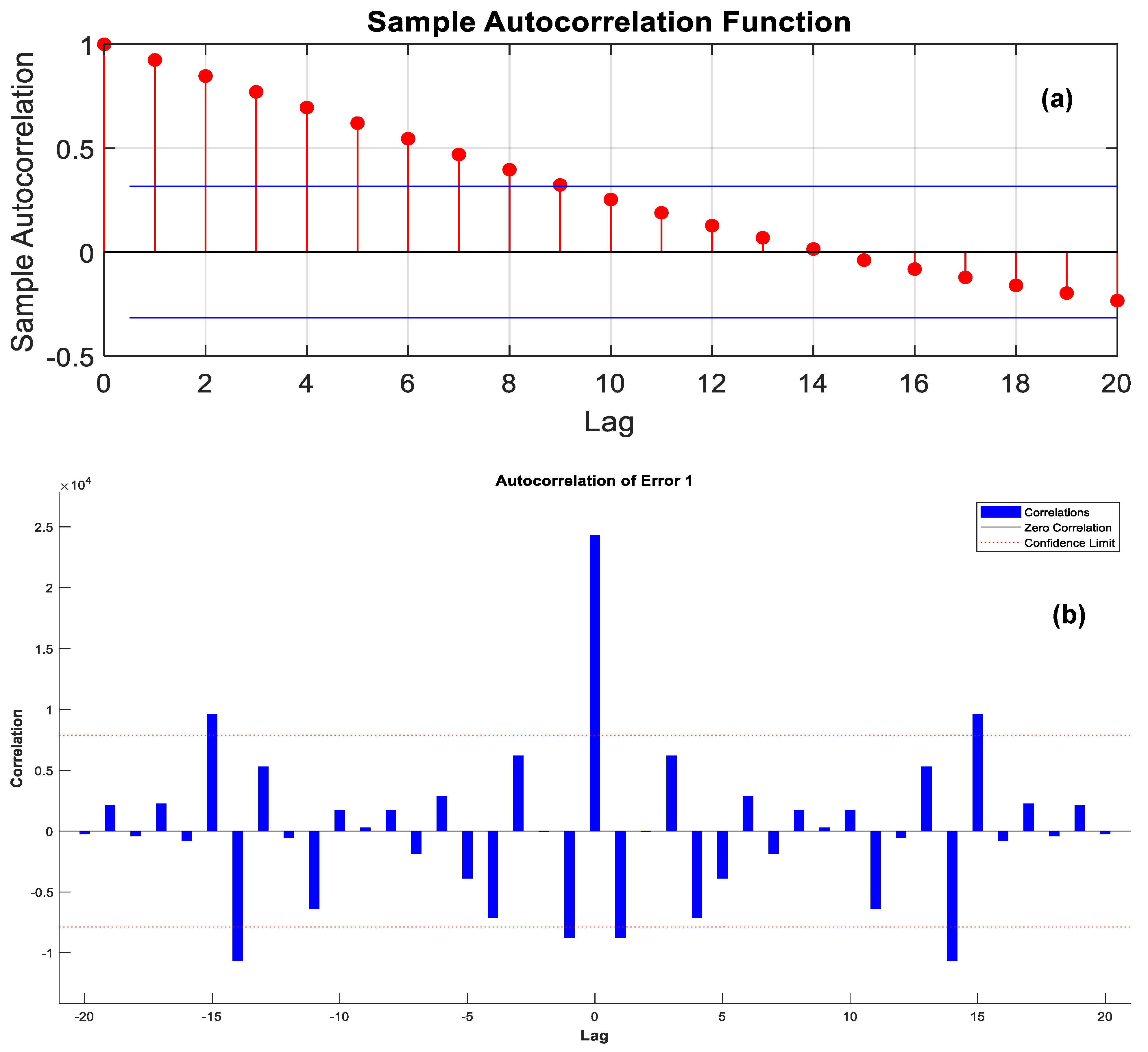
Initially, the linear time series for the worldwide electricity consumption should be statistically, visually, or algebraically checked for the unit root nonstationarity [30]. In this paper, we have visually assessed the stationarity by inspecting the plots of the sample autocorrelation function (ACF). According to Figure 4a, the downward sloping of the plot indicates a unit root process. The lengths of the line segments on the ACF plot gradually decay, and this pattern continues for increasing lags. This behavior indicates a nonstationary series. As a result, we have applied the detrending and differencing transformations that can be used to address nonstationarity due to a trending mean [31]. According to this methodology, the resultant data looks stationary, as illustrated in the plot of the sample autocorrelation function (ACF) of Figure 4b.
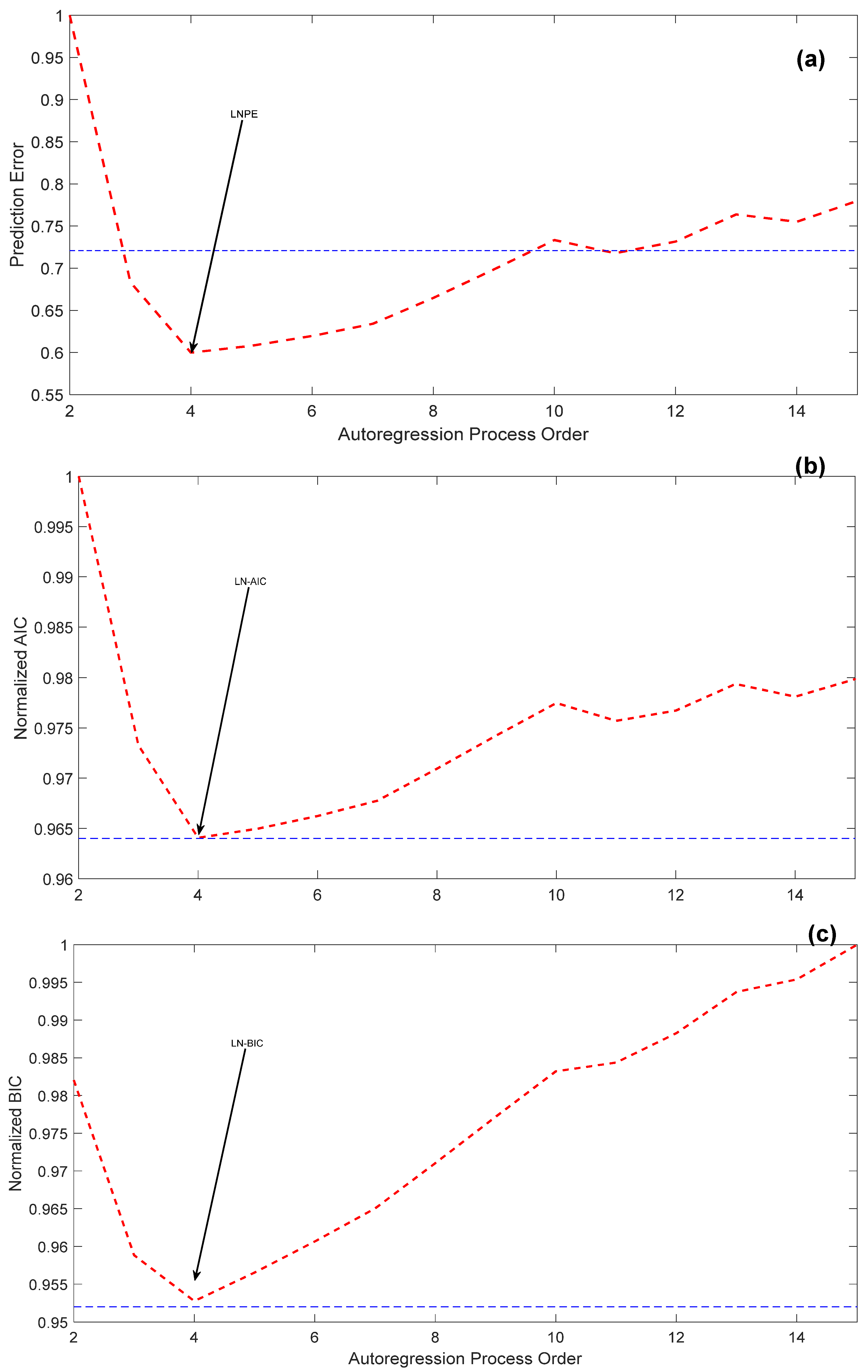
In the previous sections, we presented the genuine datasets of the yearly issues for electric energy consumption using the past data-records from 1980 to 2019. In terms of time-series reliability, we have to choose the best regression order for the AR process by illustrating the acquisitive autoregression error values vs. the autoregression order values to select the greatest order that diminishes the estimation error and lessens the design complexity as well. The cumulative (final) autoregression/prediction error can be computed using various error calculation techniques such as via the evaluation of normalized final prediction error using () for each regression order value. Therefore, the relationships among various regression/prediction order-numbers in opposition to final regression/prediction error (FPE), Akaike information criterion (AIC), and Bayesian information criterion (BIC) [32] are illustrated in Figure 4. Besides, the figure demonstrates the determination process for the best regression order number using the least accumulated error of the three measures. As a result, the fourth autoregression process order, i.e., , has been selected as the most appropriate scheme to regress and forecast the wide variety of electricity amounts’ time series as it resembles the least normalized prediction error (LNPE), least normalized Akaike information criterion (LN-AIC), and Bayesian information criterion (LN-BIC) [33]; it can reproduce the common quantity of electricity time series with highest regression confidence percentage () of more than 95.7% for the most fulfilling model order, see Figure 5.
Figure 6 demonstrates the data-records correlation for the given time series by visualizing the original time series vs. the regressed time series using process along with the regression error per sample. According to this illustration, the time-series regression for the given-dataset indicators is very specific and very close to the original dataset indicators, including a very insignificant discrepancy. The reason for having such a high level of data matching is the large degree of linearity between the data-points of the original time series. This clearly illustrates the influence of the autoregression scheme, and hence, this process can be employed to forecast the subsequent decade with extreme accuracy, peaking at 95.7% for the presented time series.
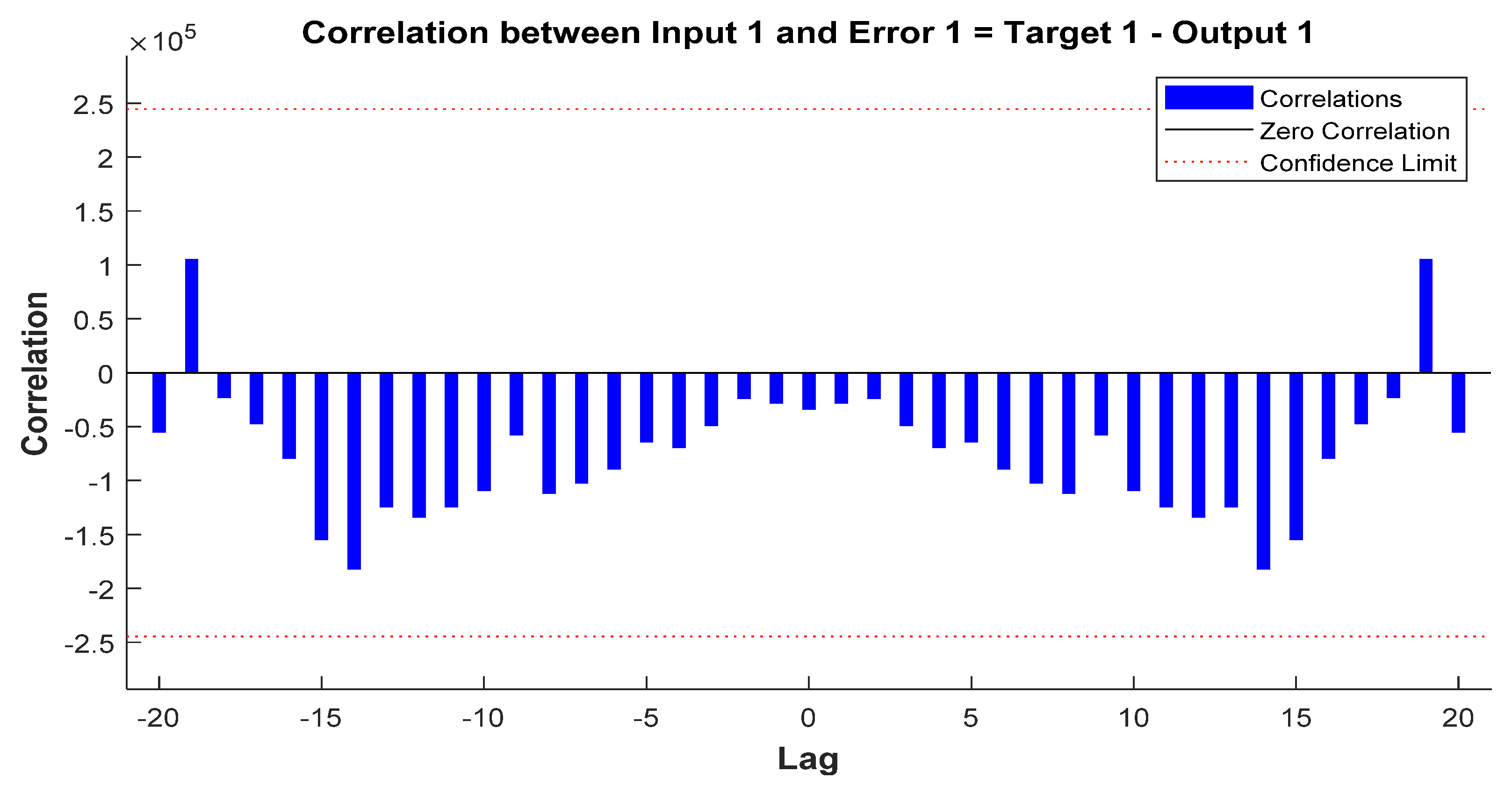
Besides, the cross-correlation function () that calculates the degree of similarity among two different signals (datasets), i.e., the dataset x and the shifted versions of a dataset y, can be used as a metric to measure the similarity between the original datasets and the regressed datasets for the aforementioned datasets. Figure 7 illustrates the input cross-correlation functions ) between the actual dataset and the regressed dataset for the electricity consumption dataset. According to the figure, the results of the reveal a high level of similarity for the examined dataset throughout the actual datasets with additional similarity spans. The simulated results appear as autocorrelation figures because the estimation models for each time sequence are fairly accurate and unique, mainly for the net electricity consumption dataset. Nonetheless, the results in Figure 6 demonstrate nonsignificant variations among the data points of the original signal values and the reproduced data points of the autoregressive process for the plot of yearly quantities of net electricity consumption which acquired lesser accuracy proportions for the regression process percentage, especially between 2005 and 2008.
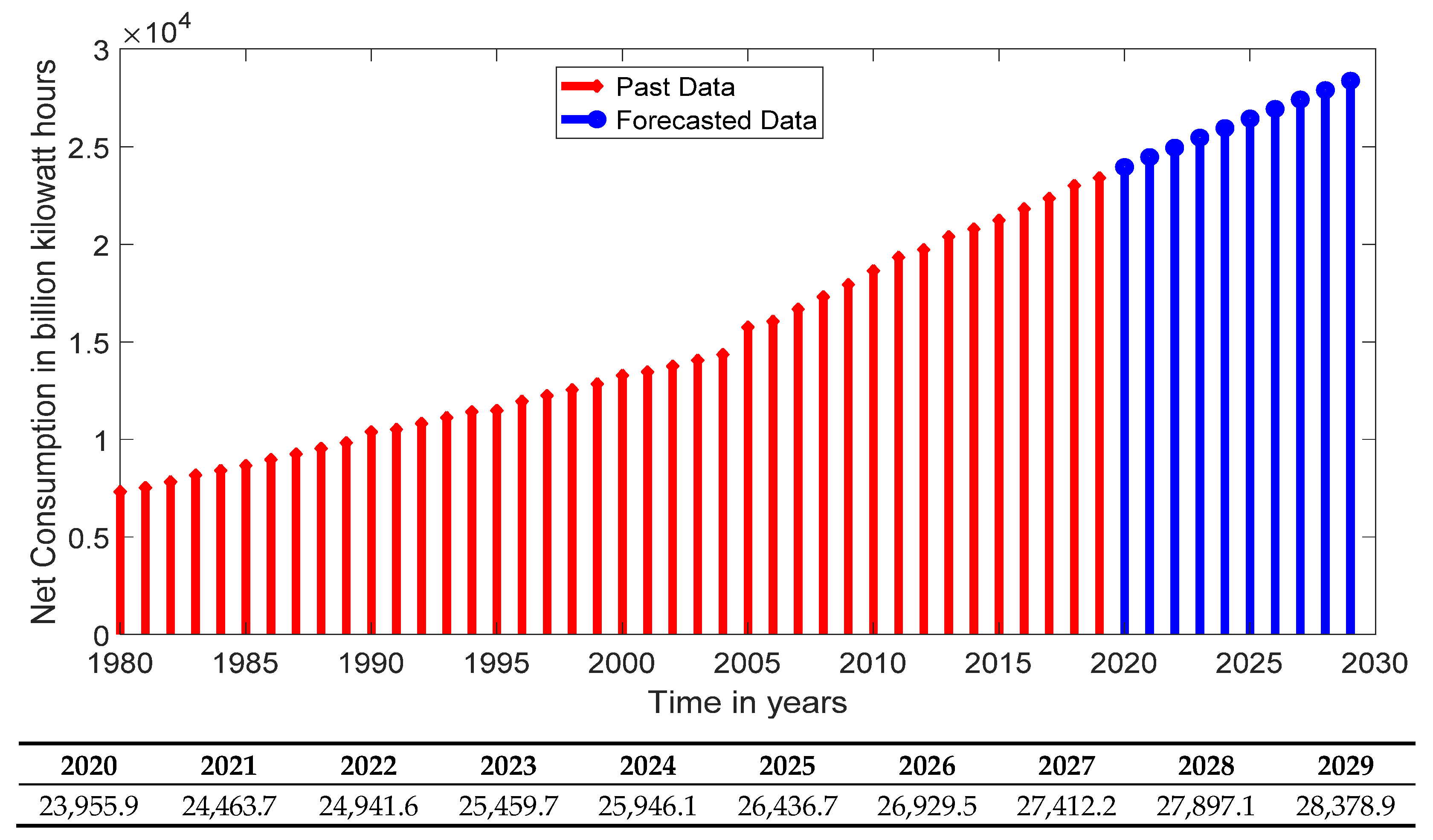
Lastly, as the resultant optimum regression process has exhibited a delicate signal prediction tool with high regression confidence percentage (RCP), we can confidently apply the resultant regression process to forecast the possible near-term forthcoming numbers for the yearly published globally accumulated amounts of electric energy consumption time series. Figure 8, along with its corresponding table, provides the potential projection of the yearly numbers for the subsequent decade (2020–2029) for the abovementioned dataset records. Accordingly, it appears that global electricity consumption will continue to grow in a linear tendency, reaching 26.4 trillion kWh in 2025 and 28.4 trillion kWh in 2029.
4. Conclusions
An autoregressive (AR) model has been developed to predict the progression of global electricity consumption using the time series of the net electricity use records released annually. The proposed system makes use of the optimum order number of the AR model derived at the lowest estimation error percentage with peak modeling accuracy. Consequently, the experimental outcomes indicated that the optimum AR modeling orders to model and forecast the provided time-series signal have verified a significant stage of confidence with a prediction self-confidence of 95.6%. As a result, the developed system has been effectively employed to forecast the forthcoming decade (2020–2029) of the growth in worldwide annual use/demand of electricity in kilowatt-hours. Accordingly, the progression ratio of the global electricity consumption amounts showed a linear increasing tendency.
Funding
This research received no external funding.
Conflicts of Interest
The author declares no conflict of interest.
References
- Liu, Z.Y. Global Energy Internet; China Electric Power Press: Beijing, China, 2015. [Google Scholar]
- International Energy Agency-IEA. Electricity Information: Overview; Statistics Report; International Energy Agency-IEA: Paris, France, 2020. [Google Scholar]
- Sönnichsen, N. Electricity consumption worldwide in 2017, by select country (in terawatt hours). Statista 2020, 21–40. [Google Scholar]
- Sönnichsen, N. Net consumption of electricity worldwide from 1980 to 2017(in billion kilowatt hours). Statista 2020. [Google Scholar]
- Enerdata. Global Energy Statistical Yearbook 2020: Electricity Domestic Consumption. Energy Rep. 2020, 6, 1973–1991. [Google Scholar]
- Liu, Z. Global Energy Development: The Reality and Challenges. In Global Energy Interconnection; Elsevier BV: Amsterdam, The Netherlands, 2015; pp. 1–64. [Google Scholar]
- Abu-Al-Haija, Q.; Smadi, M.A. Parametric prediction study of global energy-related carbon dioxide emissions. In Proceedings of the 2020 International Conference on Electrical, Communication, and Computer Engineering (ICECCE), Kuala Lumpur, Malaysia, 12–13 June 2020; Institute of Electrical and Electronics Engineers (IEEE): Piscataway, NJ, USA, 2020; pp. 1–5. [Google Scholar]
- Huang, J.; Korolkiewicz, M.; Agrawal, M.; Boland, J. Forecasting solar radiation on an hourly time scale using a Coupled AutoRegressive and Dynamical System (CARDS) model. Sol. Energy 2013, 87, 136–149. [Google Scholar] [CrossRef]
- Abu-Al-Haija, Q.; Mao, Q.; al Nasr, K. Forecasting the Number of Monthly Active Facebook and Twitter Worldwide Users Using ARMA Model. J. Comput. Sci. 2019, 15, 499–510. [Google Scholar] [CrossRef] [Green Version]
- Lydia, M.; Kumar, S.S.; Selvakumar, A.I.; Kumar, G.E.P. Linear and non-linear autoregressive models for short-term wind speed forecasting. Energy Convers. Manag. 2016, 112, 115–124. [Google Scholar] [CrossRef]
- Abu-Al-Haija, Q.; Tawalbeh, L. Autoregressive Modeling and Prediction of Annual Worldwide Cybercrimes for Cloud Environments. In Proceedings of the 2019 10th International Conference on Information and Communication Systems (ICICS), Irbid, Jordan, 11–13 June 2019; Institute of Electrical and Electronics Engineers (IEEE): Piscataway, NJ, USA, 2019; pp. 47–51. [Google Scholar]
- Abadi, A.; Rajabioun, T.; Ioannou, P.A. Traffic Flow Prediction for Road Transportation Networks with Limited Traffic Data. IEEE Trans. Intell. Transp. Syst. 2014, 16, 1–10. [Google Scholar] [CrossRef]
- Abu-Al-Haija, Q.; Al Nasr, K. Supervised Regression Study for Electron Microscopy Data. In Proceedings of the 2019 IEEE International Conference on Bioinformatics and Biomedicine (BIBM), San Diego, CA, USA, 18–21 November 2019; Institute of Electrical and Electronics Engineers (IEEE): Piscataway, NJ, USA, 2019; pp. 2661–2668. [Google Scholar]
- Ruiz, L.G.B.; Cuéllar, M.P.; Calvo-Flores, M.D.; Jiménez, M.D.C.P. An Application of Non-Linear Autoregressive Neural Networks to Predict Energy Consumption in Public Buildings. Energies 2016, 9, 684. [Google Scholar] [CrossRef] [Green Version]
- Abu-Al-Haija, Q.; al Nasr, K. Forecasting Model for the Annual Growth of Cryogenic Electron Microscopy Data. In Lecture Notes in Computer Science; Metzler, J.B., Ed.; Springer: Berlin/Heidelberg, Germany, 2020; Volume 12029, pp. 147–158. [Google Scholar]
- Nogales, F.; Contreras, J.; Conejo, A.; Espinola, R. Forecasting next-day electricity prices by time series models. IEEE Trans. Power Syst. 2002, 17, 342–348. [Google Scholar] [CrossRef]
- Costa, A.M.; Franca, P.M.; Lyra, C. Two-level network design with intermediate facilities: An application to electrical distribution systems. Omega 2011, 39, 3–13. [Google Scholar] [CrossRef]
- Tutun, S.; Chou, C.-A.; Canıyılmaz, E. A new forecasting framework for volatile behavior in net electricity consumption: A case study in Turkey. Energy 2015, 93, 2406–2422. [Google Scholar] [CrossRef]
- Abdoos, A.; Hemmati, M.; Abdoos, A.A. Short term load forecasting using a hybrid in-telligent method. Knowl. Based Syst. 2015, 76, 139–147. [Google Scholar] [CrossRef]
- Hu, Y.-C. Electricity consumption prediction using a neural-network-based grey forecasting approach. J. Oper. Res. Soc. 2017, 68, 1259–1264. [Google Scholar] [CrossRef]
- Abu-Al-Haija, Q.; Tarayrah, M.; Enshasy, H.M. Time-Series Model for Forecasting Short-term Future Additions of Renewable Energy to Worldwide Capacity. In Proceedings of the IEEE 2020 International Conference on Data Analytics for Business and Industry: Way Towards a Sustain-able Economy (ICDABI), Sakheer, Bahrain, 26–27 October 2020. [Google Scholar]
- Wang, C.H.; Hsu, L.C. Using genetic algorithms grey theory to forecast high technology industrial output. Appl. Math. Comput. 2008, 195, 256–263. [Google Scholar] [CrossRef]
- Pi, D.; Liu, J.; Qin, X. A Grey Prediction Approach to Forecasting Energy Demand in China. Energy Sources Part A Recov. Util. Environ. Eff. 2010, 32, 1517–1528. [Google Scholar] [CrossRef]
- Lee, Y.S.; Tong, L.I. Forecasting energy consumption using a grey model improved by incorporating genetic programming. Energy Convers. Manag. 2011, 52, 147–152. [Google Scholar] [CrossRef]
- Feng, S.J.; Ma, Y.D.; Song, Z.L.; Ying, J. Forecasting the Energy Consumption of China by the Grey Prediction Model. Energy Sources Part B Econ. Plan. Policy 2012, 7, 376–389. [Google Scholar] [CrossRef]
- Li, D.C.; Chang, C.J.; Chen, C.C.; Chen, W.C. Forecasting short-term electricity consumption using the adaptive grey-based approach—An Asian case. Omega 2012, 40, 767–773. [Google Scholar] [CrossRef]
- Proakis, J.G.; Manolakis, D.K. Digital Signal Processing. In Pearson, 4th ed.; Prentice-Hall: Englewood Cliffs, NJ, USA, 2007; ISBN 100131873741. Available online: https://www.pearson.com/us/higher-education/program/Proakis-Digital-Signal-Processing-4th-Edition/PGM258227.html (accessed on 22 March 2019).
- Gray, R.M. Toeplitz and Circulant Matrices: A Review. Found. Trends Commun. Inf. Theory 2005, 2, 155–239. [Google Scholar] [CrossRef]
- Al-Nasr, K.; Abu-Al-Haija, Q. Forecasting the Growth of Structures from NMR and X-Ray Crystallography Experiments Released Per Year. J. Inf. Knowl. Manag. 2020, 19, 2040004. [Google Scholar] [CrossRef]
- Palachy, S. Detecting stationarity in time series data. Medium Towards Data Sci. 2019, 9, 53. [Google Scholar]
- Box, G.E.P.; Jenkins, G.M.; Reinsel, G.C. Time Series Analysis: Forecasting and Control, 3rd ed.; Prentice Hall: Englewood Cliffs, NJ, USA, 1994. [Google Scholar]
- Brownlee, J. Probabilistic Model Selection with AIC, BIC, and MDL; in Probability; Machine Learning Mastery: San Francisco, CA, USA, 2019. [Google Scholar]
- Niedwiecki, M.; Cioek, M. Akaike’s final prediction error criterion revisited. In Proceedings of the 40th International Conference on Telecommunications and Signal Processing (TSP), Barcelona, Spain, 5–7 July 2017. [Google Scholar]
Figure 1.
The overall growth in net consumption of electricity worldwide from 1980 to 2019 (in billion kilowatt-hours).
Figure 1.
The overall growth in net consumption of electricity worldwide from 1980 to 2019 (in billion kilowatt-hours).

Figure 2.
The hardware realization of autoregressive model where Z−1 is the time shift (delay) operator; is the target model signal to be described and predicted by model; is a prediction noise (error); and a1, a2, …, ap are polynomial coefficients for model which are derived according to the model order.

Figure 3.
The structure chart for the time-series modeling approach illustrating the modeling procedure steps from scattered data points to the regularized predicted data points.
Figure 3.
The structure chart for the time-series modeling approach illustrating the modeling procedure steps from scattered data points to the regularized predicted data points.

Figure 4.
Assessment of stationarity of a time series using sample autocorrelation function (ACF) for (a) the original time series (nonstationary) and (b) the transformed time series (stationary).
Figure 4.
Assessment of stationarity of a time series using sample autocorrelation function (ACF) for (a) the original time series (nonstationary) and (b) the transformed time series (stationary).

Figure 5.
(a) Relationship between normalized prediction error and the regressing scheme order. (b) Relationship between Akaike information criterion (AIC) and the regressing scheme order. (c) Relationship between Bayesian information criterion (BIC) and the regressing scheme order.
Figure 5.
(a) Relationship between normalized prediction error and the regressing scheme order. (b) Relationship between Akaike information criterion (AIC) and the regressing scheme order. (c) Relationship between Bayesian information criterion (BIC) and the regressing scheme order.

Figure 6.
Time-series regression fit curves for the aforementioned dataset using the best possible regression order: (a) original vs. target curve; (b) regression errors (per sample).
Figure 6.
Time-series regression fit curves for the aforementioned dataset using the best possible regression order: (a) original vs. target curve; (b) regression errors (per sample).

Figure 7.
The cross-correlation functions (CCFs) for the aforementioned dataset using the best possible regression order.
Figure 7.
The cross-correlation functions (CCFs) for the aforementioned dataset using the best possible regression order.

Figure 8.
The anticipated figures for the forthcoming decade of the aforementioned dataset. Based on the statistics illustrated in the figure, the evolution ratio of the electric energy consumption numbers exhibits a linearly expanding development.
Figure 8.
The anticipated figures for the forthcoming decade of the aforementioned dataset. Based on the statistics illustrated in the figure, the evolution ratio of the electric energy consumption numbers exhibits a linearly expanding development.

Publisher’s Note: MDPI stays neutral with regard to jurisdictional claims in published maps and institutional affiliations. |
© 2021 by the author. Licensee MDPI, Basel, Switzerland. This article is an open access article distributed under the terms and conditions of the Creative Commons Attribution (CC BY) license (https://creativecommons.org/licenses/by/4.0/).
Share and Cite
MDPI and ACS Style
Abu Al-Haija, Q. A Stochastic Estimation Framework for Yearly Evolution of Worldwide Electricity Consumption. Forecasting 2021, 3, 256-266. https://0-doi-org.brum.beds.ac.uk/10.3390/forecast3020016
AMA Style
Abu Al-Haija Q. A Stochastic Estimation Framework for Yearly Evolution of Worldwide Electricity Consumption. Forecasting. 2021; 3(2):256-266. https://0-doi-org.brum.beds.ac.uk/10.3390/forecast3020016
Chicago/Turabian StyleAbu Al-Haija, Qasem. 2021. "A Stochastic Estimation Framework for Yearly Evolution of Worldwide Electricity Consumption" Forecasting 3, no. 2: 256-266. https://0-doi-org.brum.beds.ac.uk/10.3390/forecast3020016