Modeling and Forecasting Daily Hotel Demand: A Comparison Based on SARIMAX, Neural Networks, and GARCH Models

Abstract

Overnight forecasting is a crucial challenge for revenue managers because of the uncertainty associated between demand and supply. However, there is limited research that focuses on predicting daily hotel demand. Hence, this paper evaluates various models’ of traditional time series forecasting performances for daily demand at multiple horizons. The models include the seasonal naïve, Holt–Winters (HW) triple exponential smoothing, an autoregressive integrated moving average (ARIMA), a seasonal autoregressive integrated moving average (SARIMAX) with exogenous variables, multilayer perceptron (MLP) artificial neural networks model (ANNs), an sGARCH, and GJR-GARCH models. The dataset of this study contains daily demand observations from a hotel in a US metropolitan city from 2015 to 2019 and a set of exogenous social and environmental features such as temperature, holidays, and hotel competitive set ranking. Experimental results indicated that under the MAPE accuracy measure: (i) the SARIMAX model with external regressors outperformed the ANN-MLP model with similar external regressors and the other models, in every one horizon except one out of seven forecast horizons; (ii) the sGARCH(4, 2) and GJR-GARCH(4, 2) shows a superior predictive accuracy at all horizons. The results performance is evaluated by conducting pairwise comparisons between the different model’s distribution of forecasts using Diebold–Mariano and Harvey–Leybourne–Newbold tests. The results are significant for revenue managers because they provide valuable insights into the exogenous variables that impact accurate daily demand forecasting.

1. Introduction

Over the past several years, the rapid development of information technology has been instrumental in the growth of demand in the hospitality sector. The new marketplace is becoming more competitive, which causes pricing pressure on the traditional service industries as the market supply increases. Moreover, with this increase in prominent destinations supply, and the number of new accommodation listings beyond the traditional purchasing options (e.g., sharing accommodation), new challenges on overnight demand related to forecasting have been created. These new business models brought dramatic changes to the sales processes. Consequently, forecasting demand as an essential function for the hospitality industry stakeholders has developed new interesting forecasting models. To this point, although accurate forecasting is a critical component that affects revenue maximization when selecting a specific model, the model choice within forecasting is crucial in itself. For example, a reduction of the forecasting error might generate incremental revenue.

This study focuses on forecasting overnight demand by studying approaches to predict daily demand. Recent literature, see [1,2,3], has looked at various techniques to examine the accuracy of hotel occupancy forecasts. Historically, each recommended method demonstrates drawbacks [4] since many estimates use historical patterns to predict future estimation. At the same time, the market challenges the standards for determining forecasting techniques and accuracy indicators, the length of the forecast horizon, and the level of accuracy uncertainty [5]. This leads to strong irregularity, along with seasonal patterns. The overnight demand exhibits variant arrival behavior that may contain outliers due to factors such as promotions, holidays, and citywide events. In this context, the different types of datasets often incorporate daily, intra-week, weekly, monthly, and even intra-year irregular behavior that provides curves with trend and seasonality. Therefore, daily demand structures are influenced by the strong effects of outliers, which, adjusting and transforming to simplify the pattern, can often lead to a more accurate forecast.

The models employed in most of the existing hospitality and tourism literature for the demand modeling and forecasting purposes include the vector autoregressive models (VAR and VECM) or Bayesian technique (BVAR), autoregressive moving average (ARIMA), exponential smoothing (ETS), time-varying parameter models (TVP), TBATS, choice modeling, and, recently, more advanced machine learning (ML) models (see [3,6,7,8,9,10,11,12,13,14,15,16]). Genuinely, in modeling, seasonality is usually examined by the seasonal autoregressive integrated moving average (SARIMA) model, which has been proven to have better performance [5]. There is applied research on forecasting daily or intraday high-frequency data in the operation of call centers and finance (see [17,18]). Call centers face daily high call volumes, while arrival calls demonstrate complex trends and seasonal cycles [19]. Nowadays, consumer behavior and market observations justifying those daily forecasting procedures should be adjusted to trends and demand variations incorporating data that strongly affect demand. Hotel demand exhibits high trends and seasonal patterns with an annual seasonal pattern influenced by external factors, and from a first view, traditional hotel revenue management forecasting is no longer entirely applicable. Likewise, daily hotel demand exhibits several seasonal effects such as weekly pattern, intra-week, and weekend pattern with a period of seven days and low, medium. Therefore, due to the nature of complexity, there is limited research on the hotel demand topic while employing high-frequency daily data.

This paper aims to form an understanding for revenue managers of the existing forecasting methods and reveal what can be implemented in practice. A short theoretical outline about the implemented forecasting methods will be represented in detail to show the revenue managers that only a small portion is implemented in the daily hotel operations. This shows the gap present between the theory and practice used in the hotel operation. Therefore, due to the great interest in advanced forecasting models, the goal is to measure how successful neural network models (ANN), seasonal ARIMAX (SARIMAX), GARCH (sGARCH), and Glosten–Jagannathan–Runkle GARCH (GJR-GARCH) models perform comparably to simple alternatives. Asymmetric GARCH models such the GJR-GARCH [20] have shown superior predictive out-of-sample performance. We evaluate the performance of these models with alternative prediction approaches, including a seasonal naïve method, a Holt–Winters (HW) triple exponential smoothing model, and an autoregressive integrated moving average (ARIMA) model. In addition, we implement exogenous indicators (temperature, holidays, and hotel competitive set ranking) to the SARIMAX and the multilayer perceptron (MLP) model, a neural network model (ANN). Moreover, we conduct pairwise comparisons between the different model’s distribution of forecasts using Diebold and Mariano (1995) [21] and Harvey–Leybourne–Newbold (1997) [22].

We recall that demand levels typically exhibit multiple fluctuations daily due to the strong effects of the exogenous indicators. Accurate forecasts are essential for revenue managers as the entire hotel operation of each department depends heavily on their estimations of demand and prices. Hence, an analysis of specific metrics has been introduced to measure forecast accuracy, namely, the Mean Absolute error (MAE), the Root Mean Square Error (RMSE), and the Mean Absolute Percentage Error (MAPE). Mainly, we evaluate if the improvements achieved in the empirical results will indicate more robust predictions for the overnight demand as the revenue management team relies on accuracy improvements. Lastly, we considered the ANN-MLP as the benchmark forecasting model; thus, we measure the accuracy along each model forecasts using the Relative Mean Absolute Percentage Error (rMAPE) and the Relative Root Mean Square Error (rRMSE) measure. More specifically, we evaluate if the proposed model will confirm the literature, implying the effectiveness of neural network models towards comparative statistical models. A dataset of 1484 daily demand observations from a major hotel throughout December 2015 to December 2019 is examined. Our results show that the multilayer perceptron neural network model, including exogenous variables, is not favorable compared to the SARIMAX model, including the same exogenous variables such as temperature, holidays, competitive set ranking, or the GARCH models.

The study results can be summarized as follows: (i) the SARIMAX model with external regressors is generally favorable and yields better results than the other models, including the ANN-MLP model with similar external regressors, in every one horizon except one out of seven forecast horizons; and (ii) the sGARCH-sttd and GJR-GARCH-sged shows a superior predictive accuracy at all horizons. Both GARCH models have a high predictive ability at the short and long horizons.

The paper is organized as follows: Section 2 presents a short review of the current literature, while Section 3 follows an explanation of the model estimation and analysis of the study results, highlighting the applied techniques and further discussion. Finally, Section 4 summarizes the paper’s conclusions and possible future research.

2. Evaluation of Forecasting Methods

Before describing the empirical study results of the dataset, this chapter outlines the various forecasting methods employed in the study. It provides an explanation and details of each method. This is an empirical study, and it is crucial to show to the revenue managers how the forecasting methods have developed and evolved during the last several years and the advantages and disadvantages of each method.

Different types of econometric models are frequently employed to perform demand forecasting. The traditional methods of quantitative forecasting include the time-series domain, which is a set of observations generated sequentially in time and can be described by its stationarity (mean, variance, and autocorrelation function) [23,24]. Forecasts made at t time are needed at some future time $t+l$, that is, at lead time l, which vary with each problem and properties on an objective to obtain a probability accuracy small as possible based upon the actual and forecasted values [23].

In particular, several methods have been proposed in the hotel forecasting literature. Traditional time-series models such as exponential smoothing, moving averages, and regression and more advanced models such as ARIMA in various forms have been applied for forecasting and are well proved to be efficient. These statistical models usually exercise historical databases; however, the outcome is under the prerequisite that selects the appropriate parameters. In light of the advanced algorithm modeling, artificial neural networks (ANN) have shown impressive results in developing forecasting models for other industries; hence, we also implement this study.

2.1. Seasonal Naïve Method

The seasonal naïve approach is an advanced naïve benchmark model for forecasting series with highly seasonal data. It states that each forecast should be equal to the last observed value from the same season. The forecast for time $T+h$ is written as ${\widehat{y}}_{T+h}=y_{T+h-m}$, where $y_T$ is the demand at the hotel at period $T=1\cdots ,n$, h is the forecast horizon, m is the seasonal period, and ${\widehat{y}}_T$ is the forecasted demand [24]. For example, with daily data, the forecast for all future days within a specific month value equals the last observed similar monthly day value. Even nowadays, the naïve method is the most applicable method in the hospitality industry, referred to by revenue managers as the “Same day, last year” forecasting approach. A recent study by [3] indicated that the performance of the naïve approach was corresponding similarly to advance methods in all cases.

2.2. Holt–Winters’ Triple Exponential Smoothing

The exponential smoothing (ETS) approaches are utilized to model time series various components such as the trend, cycle, seasonal, and irregular or error (E) components [25]. ETS is an extension to the moving average method except that it is forecasting using a weighted average of all past values. The choice of the proper ETS model is determined by information criteria, such as the Akaike Information Criterion (AIC). For ETS models, AIC is defined as $\mathrm{AIC}=-2log\left(L\right)+2k$, where L is the likelihood of the model and k is the total number of parameters.

Although the ETS framework refers to the three components: error, trend, and seasonality, fitting a model with a daily seasonal cycle would need to be highly optimized, which leads to high optimization challenges. The Holt–Winters method is an extended exponential smoothing method for the time series dataset, including trends and multiple seasonal cycles. There are two types of seasonality, that is, additive and multiplicative. Ref. [26] proposed a Holt–Winters exponential smoothing designed to capture triple seasonal cycles, which are used in this paper:

$${\ell }_x=\alpha (y_x-s_{x-L})+(1-\alpha )({\ell }_{x-1}+b_{x-1})\hspace{1em}\hspace{1em}\mathrm{level}$$

(1)

$$b_x=\beta ({\ell }_x-{\ell }_{x-1})+(1-\beta )b_{x-1}\hspace{1em}\hspace{1em}\hspace{1em}\hspace{1em}\hspace{1em}\hspace{1em}\mathrm{trend}$$

(2)

$$s_x=\gamma (y_x-{\ell }_x)+(1-\gamma )s_{x-L}\hspace{1em}\hspace{1em}\hspace{1em}\hspace{1em}\hspace{1em}\mathrm{seasonal}$$

(3)

$${\widehat{y}}_{x+m}={\ell }_x+m{b}_x+s_{x-L+1+(m-1)}\hspace{1em}\hspace{1em}\hspace{1em}\hspace{1em}\hspace{1em}\mathrm{forecast}$$

(4)

where y is the observation, ℓ, b, and s model the respective series components of level, trend, and seasonality at time x and $\widehat{y}$ is the forecast for m periods ahead. The value of the parameters $\alpha$, $\beta$, and $\gamma$ are estimated from the fitting of the smoothing equation with the training data.

2.3. ARIMA

The Autoregressive Integrated Moving Average (ARIMA) model expresses an ARMA linear model class in statistical forecasting, even though exponential smoothing models are built on a capture of the trend and seasonality in the data [18], with ARIMA models defining stationary, non-stationary, and seasonal processes of order ($p,d,q$).

A common barrier in adopting Autoregressive Integrated Moving Average (ARIMA) models for forecasting is that the order selection process is usually treated as subjective and challenging to apply [24]. In this context, there have been several attempts to automate ARIMA modeling in the last years. Specifically, in the hospitality industry, seasonality also produces significant sales volatility. As a result, the forecasting procedures include the autoregressive integrated moving average (ARIMA) process as:

$$(1-{\varphi }_{1}B)(1-{\Phi }_1{B}^4)(1-B)(1-B^4)y_t=(1+{\theta }_{1}B)(1+{\mathsf{\Theta }}_1{B}^4){\epsilon }_t,$$

(5)

In the ARIMA model, to deal with multiple seasonality, external regressors need to be added [27]. In addition, to incorporate multiple seasonality Fourier terms, various external regressors are added to the ARIMA model, where $N_t$ is an ARIMA process:

$$y_t=\alpha +\sum _{i=1}^M\sum _{k=1}^{K_i}[\alpha sin\left(\frac{2\pi kt}{p_i}\right)+\beta cos\left(\frac{2\pi kt}{p_i}\right)]+N_t,$$

(6)

In this study, we have determined seasonality while considering external variables. A SARIMA model with external regressors is referred to as SARIMAX $(p,d,q){(P,D,Q)}_s$, where $p,d$ and q are the order of AR autocorrelation, the degree of difference, and the order of the moving average part, respectively, extended by $P,D$ and Q to handle seasonality, which is referred to as the seasonal part of the model, and s is the number of periods per season [28]. Moreover, we consider s = 7 because the period is one (1) week. SARIMAX models’ general form can be modeled as:

$${\varphi }_p\left(B\right){\mathsf{\Phi }}_p\left(B^s\right){\nabla }^d{\nabla }_s^D{y}_t={\beta }_k{x}_{k,t^{{}^{\prime }}}+{\theta }_q\left(B\right){\mathsf{\Theta }}_Q\left(B^s\right){\epsilon }_t,$$

(7)

where B refers to the backward shift operator $B^j$$z_t=z_{t-j}$, the integer s is the seasonal period, $x_{k,t^{{}^{\prime }}}$ is the vector including the kth explanatory input variables at time t, and ${\beta }_k$ is the coefficient value of the kth exogenous input variable. ${\nabla }^d$ and ${\nabla }_s^D$ are the non-seasonal and seasonal difference operators of order d and D, respectively.

ARIMA models can be fitted to both seasonal and non-seasonal data. Seasonal ARIMA demands a more detailed specification of the model composition. Therefore, before determining the estimation of the time series models, we performed the augmented Dickey–Fuller (ADF) [29] test, which could determine whether the dataset series are stationary; if the series is non-stationary, a data transformation is necessary. The ADF statistic is obtained by $\Delta x_t={\alpha }_0+b_0{x}_{t-1}+{\displaystyle \sum _{i=1}^k}{c}_0\Delta x_{t-1}+w_t$ where $\Delta$ is the difference operator, ${\alpha }_0$, $b_0$, and $c_0$ are coefficients to be estimated, and x is the variable whose time series properties are examined and w is the white-noise error term. In addition, the null and the alternative hypotheses are respectively $b_0$ = 0 (series is non-stationary) and $b_0$ < 0 (series is stationary). The ADF test results indicates that the data are non-stationary (7-day seasonality) with p-value being 0.076690, test statistic = −2.684889, Lag order = 24. Therefore, to generate a robust model estimation of the SARIMAX models, we should differentiate our variables, including the exogenous. Following the differentiation, we conclude that the process is stationary; thus, the null hypothesis is rejected at the 1% level.

In order to supplement the above, we followed the methodology by computing a Kwiatkowski–Phillips–Schmidt–Shin (KPSS) test (KPSS Level = 2.665255, Truncation lag parameter = 22, p-value = 0.01). In addition, we followed the methodology by [30] by computing an Osborn, Chui, Smith, and Birchenhall (OCSB) test of seasonality [31] to determine whether it needs seasonal differencing. Test statistic: −22.7428, 5% critical value: −1.6662 Lag order 7 was selected using AIC. Finally, we employed the Shapiro–Wilk (SW) test for normality, showing that none of the variables are normally distributed [32]. The determination method of the seasonal (P, D, Q) and non-seasonal (p, d, q) terms was based mainly on specific information criteria (AIC). In addition, the autocorrelation function (ACF) and partial autocorrelation function (PACF) plots were also observed and could help us determine the orders we choose in ARMA; therefore, the most fitting candidate models were selected.

2.4. Artificial Neural Network

Artificial Neural Networks (ANN) describe a fundamental class of nonlinear models. The big-data era and computational capacity have been successfully implemented into the advancement of the ANN model forecasting applications for the estimation of demand [33]. An empirical application of ANNs has demonstrated satisfactory forecasting performance with evidence mainly published in other industries than in hospitality. Therefore, ANN models have been popular in forecasting literature in various industries, with several examples coming from electricity forecasting and forecasting tourism demand between the researchers. Specifically, in hotel demand literature, the work by [34] has been one of the earliest using such models. Several ANN models have been applied to tourism and hotel forecasting practices. For a detailed presentation of an overview, the reader is referred to work by [35], which is a review of published studies from 2007 to 2015 on tourism and hotel demand modeling and forecasting methods, including studies in the neural network’s method. Nevertheless, the studies focused on hotel demand are relatively limited in employing the ANN model in relation to tourism studies.

This section and the rest of the paper focus on the most common type of ANN model, a feedforward neural network, the Multilayer Perceptrons (MLP). The MLP networks contain a set of inputs (${\rho }_i\cdots {\rho }_n$), three or more layers of neurons with a nonlinear activation function while being used in a variety of problems, especially in forecasting because of their inherent capability of arbitrary input–output mapping [33]:

$${\widehat{y}}_t={\beta }_0+\sum _{h=1}^H{\beta }_{h}g\left({\gamma }_{0i}+\sum _{i=1}^I{\gamma }_{hi}{\rho }_i\right),$$

(8)

where ${\widehat{y}}_t$ is the output vector at time t, I refers to the inputs ${\rho }_i$ number, as lags of the series, and H indicates the hidden nodes number in the neural network. The weights $w=(\beta ,\gamma )$, with $\beta =[{\beta }_1,\cdots ,{\beta }_H]$ and $\gamma =[{\gamma }_{11},\cdots ,{\gamma }_{H1}]$ are for the hidden and output layer, respectively. Similarly, the ${\beta }_0$ and ${\gamma }_{0i}$ are the biases of each node, while $g(·)$ is the transfer function, which might be either the sigmoid logistic or the tanh activation function.

In the first steps to prepare a forecast using ANNs modeling, we need to determine the applicable input variables, hidden layers, and nodes number, and select a suitable database. Finally, the neural network is trained by modifying the network is hidden and output weights to reduce the output errors on a set of training data.

2.5. GARCH Models

The ARCH (autoregressive conditional heteroscedasticity) introduced by Engle (1982) [36] and the GARCH (generalized autoregressive conditional heteroscedasticity) family of models proposed by Bollerslev (1986) [37] have been extensively utilized in the field of financial modeling to model the volatility of financial returns. The GARCH model is a continuation of the ARCH model that supports the conditional variance to change over time as a function of past errors leaving the unconditional variance constant [37]. In the hospitality industry, the application is limited to a few studies to model the demand for hotel rooms. For example, Divino and McAleer (2010) [38] used the generalized ARCH (GARCH) and the exponential GARCH to estimate the increased rate of daily arrivals to Peru. Among these studies, for example, the GARCH and Glosten–Jagannathan–Runkle GARCH (GJR-GARCH) volatility models have been applied to estimate monthly international tourism arrivals in Chan et al. (2005), Shareef and McAleer (2008), and Liang (2014) (see [39,40,41]).

A GARCH(m,s) model extends the ARCH model with a recursive term on ${\widehat{\sigma }}_t^2$:

$${\widehat{\sigma }}_t^2=\widehat{\omega }+\sum _{i=1}^m{\widehat{\alpha }}_i{w}_{t-i}^2+\sum _{j=1}^s{\widehat{\beta }}_j{\widehat{\sigma }}_{t-j}^2$$

(9)

where m is the model order, and $\omega >0,{\alpha }_i\ge 0,{\beta }_j\ge 0$ were the parameters with unconditional variance given ${\sum }_{i=1}^m{\alpha }_i+{\sum }_{j=1}^s{\beta }_j\le 1.$

The Glosten–Jagannathan–Runkle GARCH (GJR-GARCH) model assumes a specific parametric form for this conditional heteroskedasticity. Specifically, the ${ϵ}_t$ GJR-GARCH indicates ${ϵ}_t={\sigma }_t{z}_t$, where $z_t$ is standard Gaussian and:

$${\sigma }_t^2=\omega +(\alpha +\gamma I_{t-1}){ϵ}_{t-1}^2+\beta {\sigma }_{t-1}^2$$

(10)

$$I_{t-1}:=\left\{\begin{array}{c}0\mathrm{if}{r}_{t-1}\ge \mu \hfill \\ 1\mathrm{if}{r}_{t-1}<\mu \hfill \end{array}\right.$$

(11)

The common restrictions on the parameters are $\omega ,\alpha ,\gamma ,\beta >0$. The GARCH model is a restricted version of the GJR-GARCH, with $\gamma =0$. We have chosen the best model (p and q) using the Akaike Information Criterion (AIC).

3. Empirical Evaluation and Results

3.1. Forecasting Specification and Dataset

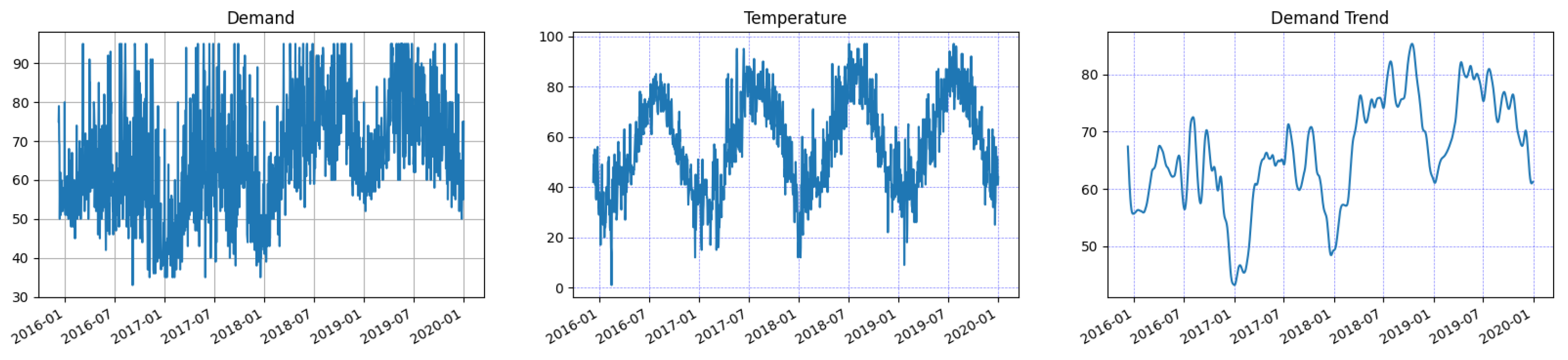
The dataset of this study contains daily demand observations for a major hotel in a US metropolitan city (Boston) over the period of 9 December 2015 to 31 December 2019. The study covers a period of 211 weeks and 4 days, including overnight demand and a set of exogenous social and environmental features (weekday, holidays, temperature, and competitive hotel ranking). Figure 1 exhibits periodic behavior of seven periods within the week and a yearly cycle. We divided the dataset into two segments, one employed for fitting the model and another for testing the out-of-sample performance following an approximate ratio of 94:6. The training set (i.e., 1391 days from 9 December 2015 to 29 September 2019) and the test set (i.e., 93 days from 29 September 2019 to 31 December 2019). We used the test set data from the end of September 2019 to December 2019 for testing the various forecasting model’s performance. The forecast horizon to observe the demand is defined from 1 to 28 days ahead forecast. In

Table 1. Descriptive statistics for dataset (December 2015–December 2019).

	n	Mean	sd	Median	Min	Max	Skew	Kurtosis	se	SW(p)
Demand	1484	66.90	14.10	66.43	33.67	95.00	0.10	−0.59	0.37	<0.01
Temperature	1484	57.44	18.66	57.00	1.90	97.00	−0.03	−0.87	0.48	<0.01
Holidays	1484	0.17	0.38	0.00	0.00	1.00	1.74	1.02	0.01	<0.01
Compsetrank	1484	4.90	2.53	5.00	1.00	10.00	−0.21	−1.16	0.07	<0.01

Note:. sd: Standard Deviation; min: Minimum; max: Maximum; skew: Skewness; se: Standard Error; SW: Shapiro–Wilk Test. Demand in %; Temperature in Fahrenheit scale.

, we report some descriptive statistics for the dataset.

In addition, to measure the accuracy of the forecasting methods, an analysis of specific metrics has been applied: the Mean Absolute error (MAE), the Root Mean Square Error (RMSE), and the Mean Absolute Percentage Error (MAPE):

$$\mathrm{MAE}=\frac{1}{h}\sum _{j=1}^h\left|y_{t+j}-{\widehat{y}}_{t+j}\right|,$$

(12)

$$\mathrm{RMSE}=\sqrt{\frac{1}{h}{\displaystyle \sum _{j=1}^h}{\left(y_{t+j}-{\widehat{y}}_{t+j}\right)}^2},$$

(13)

$$\mathrm{MAPE}=\frac{1}{h}\sum _{j=1}^h\frac{y_{t+j}-{\widehat{y}}_{t+j}}{y_{t+j}},$$

(14)

The principal means of forecasting accuracy to assess hotel demand performance, and the easiest to interpret, is the mean absolute percentage error (MAPE). RMSE is a scale-dependent measure that compares errors of different calculation models for the same forecast dataset and the eventual outcomes, while MAE is popular because of its simplicity to understand.

Finally, because we compare each model to the ANN-MLP Neural network technique, which is considered the benchmark forecasting model, we measure the accuracy of the forecasts using the Relative Root Mean Square Error (rRMSE) and the Relative Mean Absolute Percentage Error (rMAPE) measure. This way, we present a direct benchmarking between the different forecasting models to the chosen benchmarking model:

$$\mathrm{Relative}\mathrm{Root}\mathrm{Mean}\mathrm{Square}\mathrm{Error}:\mathrm{rRMSE}=\frac{{\mathrm{RMSE}}_{Metho{d}_a}}{{\mathrm{RMSE}}_{Metho{d}_b}}$$

(15)

$$\mathrm{Relative}\mathrm{Mean}\mathrm{Absolute}\mathrm{Percentage}\mathrm{Error}:\mathrm{rMAPE}=\frac{{\mathrm{MAPE}}_{Metho{d}_a}}{{\mathrm{MAPE}}_{Metho{d}_b}}$$

(16)

To measure the performance of ANN-MLP forecasts, we denote the MAPE of ANN-MLP as a denominator for all evaluations. For example, the rMAPE measure is based on relative errors, and it is not scale-dependent. Therefore, when rMAPE > 1, Method 2 is more accurate; when rMAPE < 1, the opposite is true, while, if rMAPE = 1, methods are equally accurate [42].

Moreover, to assess the statistical significance of improvements in each forecast’s forecasting accuracy, we conducted the test of predictive accuracy proposed by Diebold and Mariano (1995) [21]. Although Diebold and Mariano’s test is considered an essential measurement of forecast comparisons, it becomes less accurate for longer forecast horizons. Therefore, [22] proposed a modified Diebold–Mariano test, the Harvey–Leybourne–Newbold (HLN) test that applies to forecasts beyond one step ahead and establishes a more robust approach to assessing the differences between the performance of forecasts distribution.

3.2. Working with Outliers and Seasonality

Forecasting models can capture different types of trends or seasonal patterns. Therefore, we should examine seasonality, stationarity, and autocorrelations to propose an appropriate time series forecasting model based on specified criteria. However, forecasting models can also be affected by the magnitude outliers that produce irregularities with an impact on the state of the fitted model. Ordinarily, hotel demand is presenting with high fluctuations daily. Due to observing seasonality, for example, during the low winter and summer-fall, high season demand produces irregular pick and low patterns.

Moreover, external variables such as citywide events, promotional activities, holidays, and weather conditions can produce irregular patterns because sometimes it is difficult to identify and predict. These irregular variations presented in the form of outliers could bias the model statistics. Systematic detection and estimation to ascertain the outliers’ magnitude in historical trends can smooth the effects of the model re-estimation [43].

It can be seen that, when an outlier is observed, the forecasting model needs to be able to identify and remove such time series outliers. Referring to the work by [44], outliers vary in level or when an outlier occurred. They identified that forecasters during the detection procedure might not be able to identify the type correctly due to the nature of origin. For example, outliers that occurred near the last period of the series can not be empirically determined, and, similarly, if outliers occurred within the range of one or two periods before the forecast origin. In such cases, the behavior of outliers during the detection period, if identified, may or may not be correct.

The occupancy demand time series’s primary characteristic is irregular behavior because of seasonality, trend, and cycle. To treat such irregular curves, if they are present, the data can be seasonally deconstructed. This procedure of extracting the data behavior components is referred to as decomposition. We can decompose the series by employing either an additive or multiplicative model:

$$Y=S_t+T_t+E_t$$

$$Y=S_t\ast T_t\ast E_t$$

where $S_t$ is the seasonal component, T is the trend and cycle, and E is the remaining error. Following the dataset decomposition and, since ARIMA models require a smooth trend series to generate accurate results, further differentiation of the dataset is implemented. We can then determine p, d, and q values to fit the ARIMA model.

Finally, we ran a rolling h-step-ahead forecast, moving the estimation one step ahead of each variable to measure the out-of-sample performance. The one-step-ahead forecast continuously re-estimates the model and provides two-step-ahead forecasts, and the process continues for h periods. Based on these, we forecast the daily demand for one-day ahead prediction and continue two days to 28 days following this rolling approach. Thus, a set of h = 1- to 28-steps-ahead daily forecasts was generated.

3.3. Empirical Study

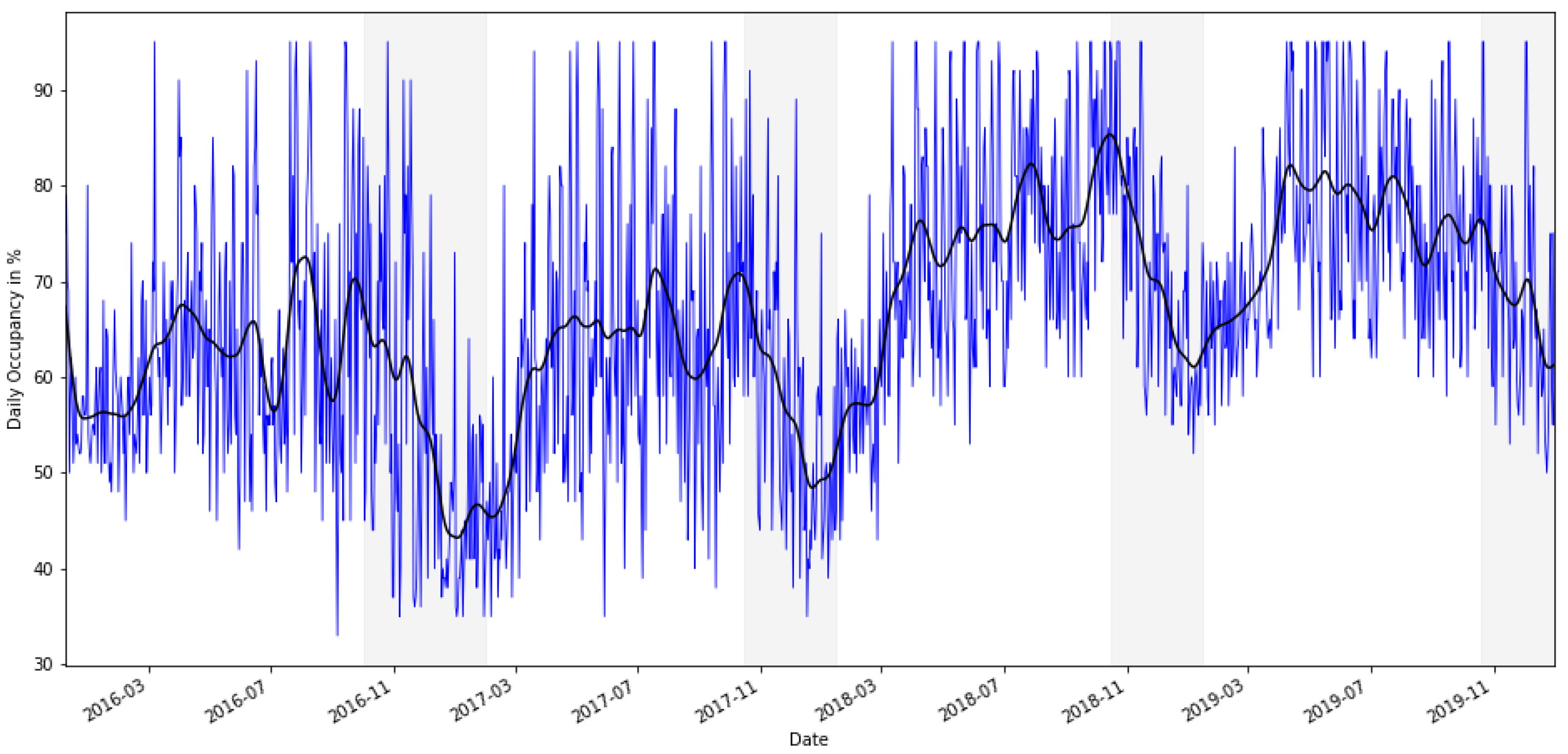
Figure 2 shows the daily demand for the entire dataset over a time period. The results indicate a stable demand over time but with a significant increase trend presented by the black line trend line. The trend shows periodic behavior within a month and year cycle. The overall mean for the monthly occupancy was 66.43% ($\mu$ = 66.43%), and the variance is 1.98%. The shaded periods show a substantial decrease in demand due to the winter period in the city. The period between March 2018 to November 2018 shows a significantly increasing trend compared to the same period last year with an average demand of 65%. The same trend continues in the year 2019. This time is considered as a low season with limited demand in any customer segment. In addition, the mean daily in the day of the week is quite similar on a daily basis, and the ratio between the variance to mean is significantly greater than one (1) every day.

In addition, Figure 1 shows the periodic behavior of temperature comparable to the series demand period. The seasonality displays a similar seasonality pattern with increases and decreases based on each period. It turns out that the temperature variable trend tends to be close to the demand series trend. Temperature is one of the exogenous factors which affects the daily demand.

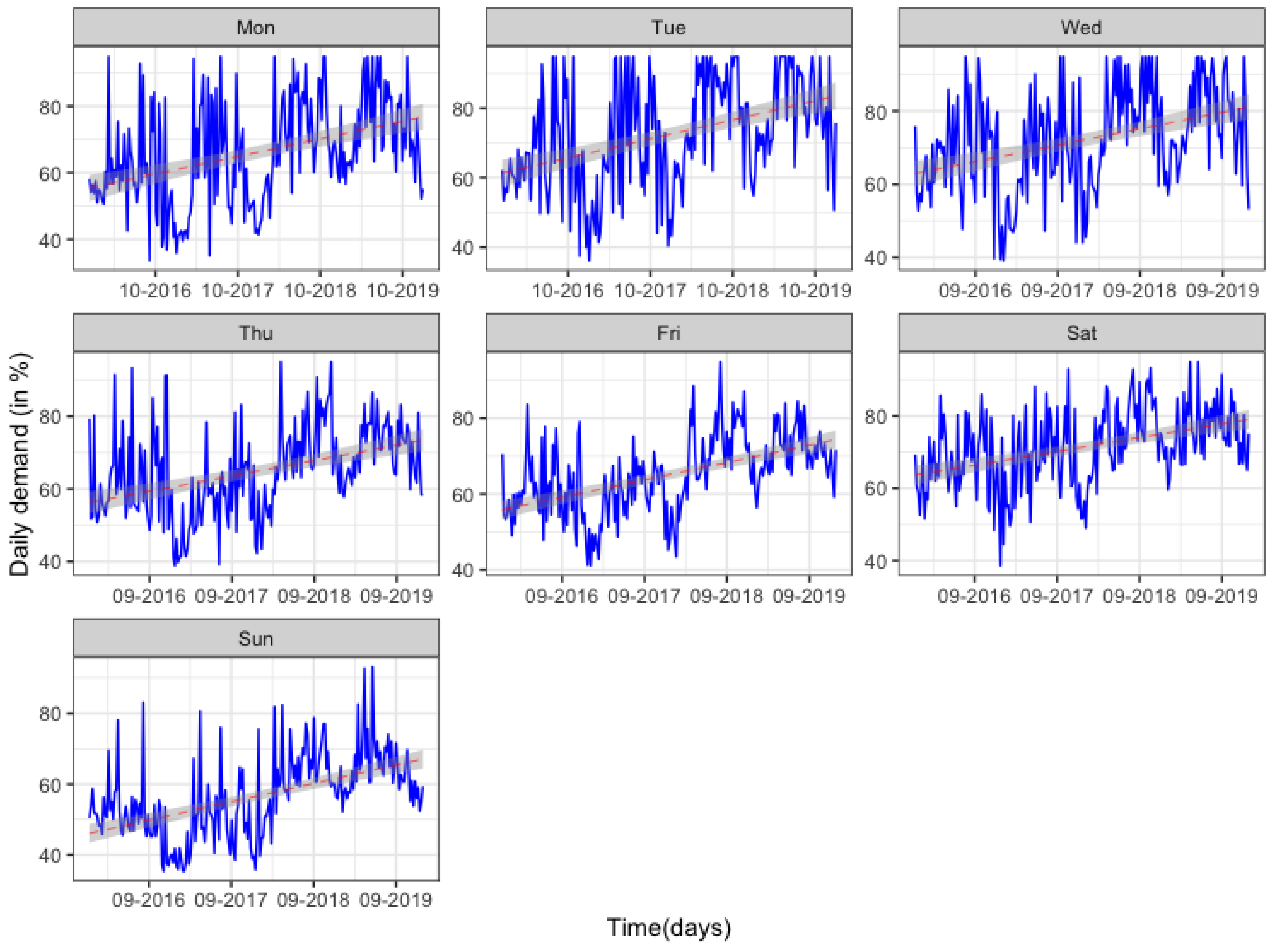
Figure 3 provides the average weekly plot of the dataset on the day of the week. The weekly seasonality indicates intraweek demand patterns. The trend shows demand fluctuation similar to business hotels, where the demand performance is higher in the middle of the week (Tuesday, Wednesday) and adjusted slightly downward on Thursday, while demand on weekends shows a decrease. In addition, the intraday of the week demand shows a considerably similar pattern with dataset demand over time. This pattern suggests that the daily demand is related to hotel type and market segment, corporate retail customers.

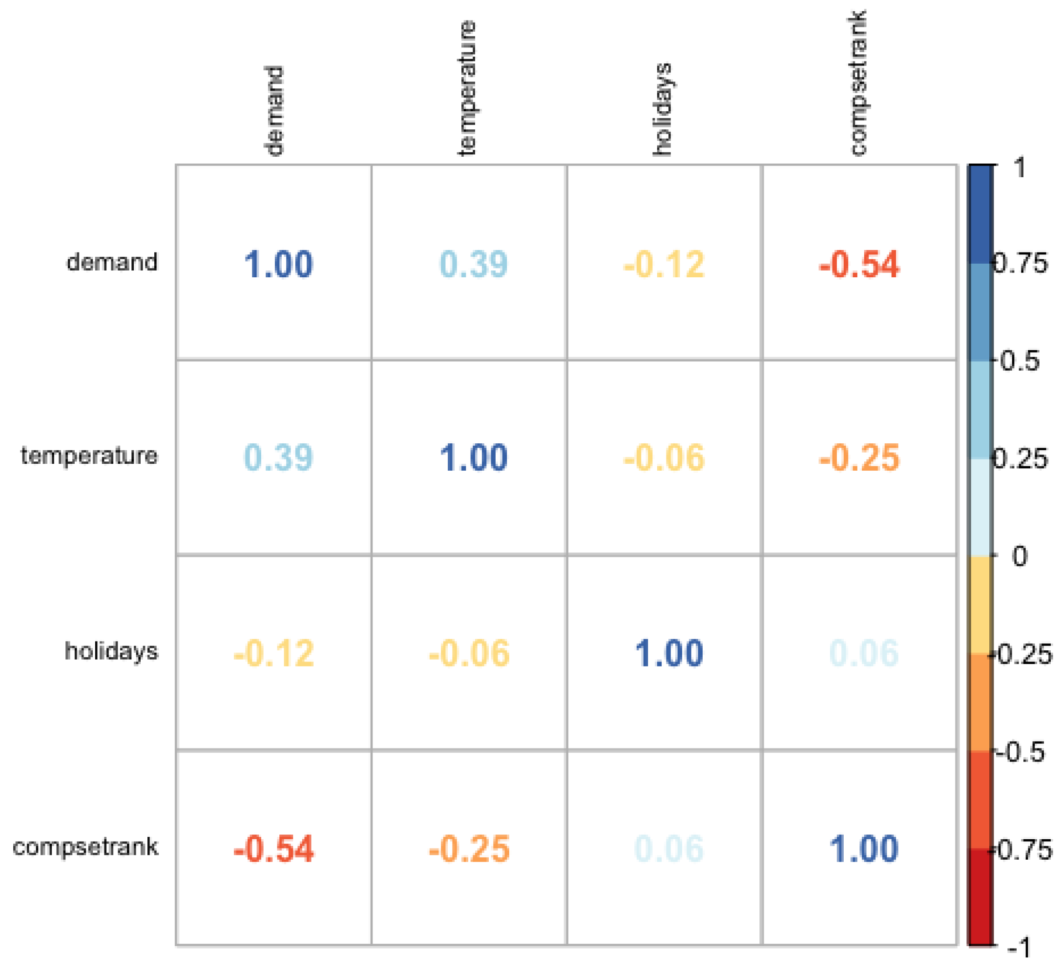
Figure 4 presents the correlation relationship among the dataset variables on each axis. The correlation values range from −1 to +1. The relationship is also symmetrical and diagonal, which can be seen because the same two variables are matched mutually in those squares.

3.4. Forecasting Methods Results

The forecast accuracy results for the four different forecast models are summarized in

Table 2. Forecasting methods’ accuracy.

Accuracy	Forecast	Forecasting Method
Measure	Horizon	SNaïve	HW	ARIMA	SARIMAX	sGARCH-sttd	gjrGARCH-sged	ANN-MLP
MAE	h = 1	6.240	8.005	5.871	8.398	2.000	2.010	3.869
	h = 2	8.650	5.009	6.799	12.131	6.465	6.455	5.269
	h = 3	9.143	6.299	7.220	16.690	5.107	5.087	5.696
	h = 7	12.031	4.354	7.570	9.864	4.761	4.761	6.009
	h = 14	11.681	4.963	7.903	11.572	4.865	4.869	8.632
	h = 21	11.099	6.142	7.535	8.371	6.547	6.537	8.456
	h = 28	11.536	7.328	7.355	12.305	7.133	7.122	8.488
RMSE	h = 1	6.240	8.005	7.313	10.365	2.000	2.010	3.869
	h = 2	7.610	7.505	8.617	14.579	4.929	4.924	4.661
	h = 3	8.199	7.338	9.290	18.866	5.473	5.463	5.054
	h = 7	9.588	7.027	9.664	12.362	5.983	5.980	6.063
	h = 14	11.595	6.562	9.963	14.437	6.042	6.039	7.388
	h = 21	12.274	6.420	9.792	10.288	6.541	6.536	8.059
	h = 28	12.683	6.527	9.201	15.214	7.259	7.251	8.341
MAPE	h = 1	9.905	12.706	12.101	8.159	2.595	2.608	6.005
	h = 2	12.134	7.661	7.379	5.961	7.914	7.902	7.305
	h = 3	12.207	8.716	9.823	5.346	6.363	6.337	7.503
	h = 7	17.781	6.080	8.008	4.146	6.649	6.652	8.374
	h = 14	16.724	6.647	9.405	5.116	6.498	6.507	11.706
	h = 21	15.622	8.100	10.563	5.093	8.213	8.204	11.277
	h = 28	15.997	9.232	11.912	5.988	8.855	8.844	11.210

Note:. MAE: Mean Absolute Error; RMSE: Root Mean Square Error; MAPE: Mean Absolute Percentage Error. MAE, RMSE in points, MAPE in percentage (%).

. An initial review of the forecasting accuracy estimates disclosed that the differences in forecast accuracy within the models are moderate. On the other side, the gap between the first and the last horizon and the remaining forecast horizons (i horizons) generated substantial differences. It is obvious that accuracy measures generate conflicting results not only between the forecasting methods but also within the examined horizons. The model with the highest performance is highlighted in boldface across the horizons. The various forecasting models out of sample performance was measured for multi-step forecasts from 1 to 28 horizons considered necessary for the hotel revenue manager (horizon: 1, 2, 3, 7, 14, 21, 28 days ahead) using a rolling approach.

Results presented in Table 2 show inconsistency along with the forecasting methods and accurate estimates. The above confirms the work of [4], which noted that each model demonstrates drawbacks, besides the criteria for choosing forecasting methods, accuracy measures, and forecast-horizon [5]. The findings indicate that forecasting with the Holt–Winters Seasonal Exponential Smoothing including a trend component and a seasonal component state-space additive model and additive errors with a no Box–Cox transformation was the best model minimized the AIC statistic with parameterization results as $\alpha$ = 0.9590, $\beta$ = 0.0046, $\gamma$ = 0.0324, and AIC = 6178.4534. In addition, the model reported more robust results in MAE and RMSE for four out of seven horizons.

According to the Akaike information criterion (AIC), ARIMA (3, 0, 5) is the best model, whose AIC is 10,784.483. Although the model partially generated promising results, the other forecasting methods such as SARIMAX, Holt–Winters, and, in some cases, the ANN-MLP models outperformed the ARIMA model. The initial analysis further showed that the Seasonal Naïve method was the least accurate approach overall.

Interestingly, the SARIMAX(1, 0, 1)(0, 1, 2, 7) model, whose AIC is 10,143.059, includes the exogenous variables as external regressors, namely temperature weekday, holidays, and competitive set ranking, it turns out that it is the best one. We employed our fitted SARIMAX model on the test set and obtained that the test MAPE is 7.333%, which is significantly more robust than any other proposed model. Table 2 reports that, based on the mean absolute percentage error (MAPE) accuracy, the SARIMAX model outperforms the others while ANN-MLP and Holt–Winters are second best. This is a significant observation considering that the ANN-MLP models are typically regarded as models that outperform most traditional models.

In addition, we considered the multilayer perceptron (MLP) model. In the neural network training, we have tried different models with hidden layers, and the number of hidden neurons ranges from 2 to 12. We run our neural network and generate our parameters multiple times to find hidden layers that generate better accuracy results. Finally, we selected the best model based on the cross-validation error (17.4564) with two hidden layers. In addition, we used all exogenous variables fitted into the ANN-MLP model similar to SARIMAX. We yielded 92.19% classification accuracy in this neural network model using a (7, 2) hidden configuration. We observe that ANN-MLP mostly outperformed all other models according to the RMSE measure for the first four out of seven horizons. It seems that, for short-term horizons (h: 1, 2, 3, 7), the ANN-MLP generates more robust results. Similarly, for MAE and MAPE, the model forms better accuracy on horizons 1 and 3 for the former and horizon 1 for the latter. Table 2 summarizes the indicative ANN model accuracy results on the three measures.

Estimation of the GARCH models was conducted via the AIC criterion. Akaike information criterion (AIC) aims to find the best prediction. For GARCH models, the results are superior to any other models in terms of the accuracy measures, including the ANN-MLP benchmark model at almost every horizon, except between sGARCH-sttd, GJR-GARCH-sged, and SARIMAX models considering the MAPE measure. These findings are in line with Divino and McAleer (2010) [38] that the GARCH models fit the data extremely well, and the estimated models were able to observe the volatility persistence of international tourist arrivals in Peru. The GARCH models are providing better forecasts among each model at h = 1 step-ahead. Moreover, in the long-term forecasts, the GARCH models are significantly better than the Seasonal Naïve, ARIMA, and ANN-MLP models (see Table 2).

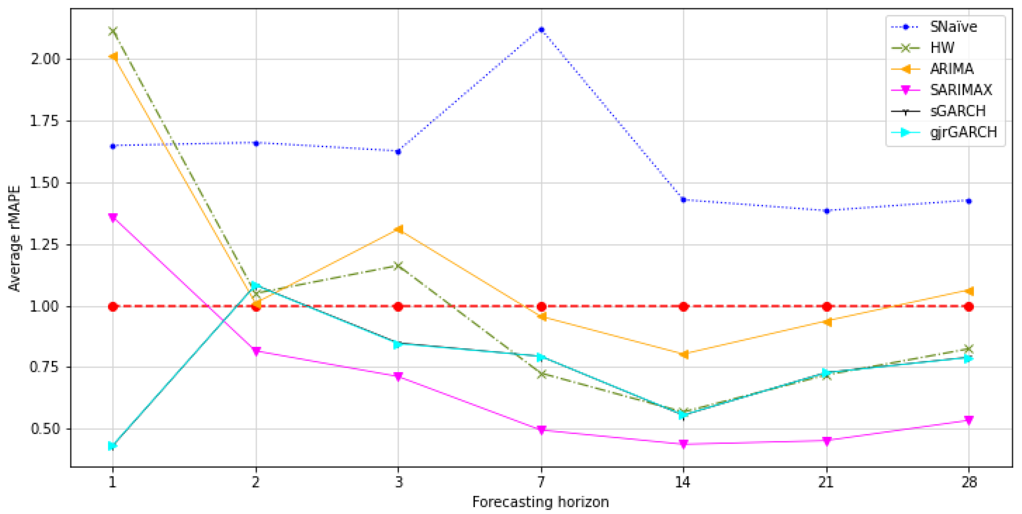
In this context, observations from the average rMAPE revealed that ANN-MLP outperformed the various models only in one (h = 1) out of seven forecast horizons, except the GARCH models while, for the remaining periods, SARIMAX following by the GARCH family models, and partially ARIMA and the Holt–Winters method perform best, verifying that seasonal methods can outperform more advanced as examined by [26]. The overall accuracy for the out-of-sample performance is demonstrated in

Table 3. Average rMAPE of forecasting methods.

Forecasting Method	h = 1	h = 2	h = 3	h = 7	h = 14	h = 21	h = 28
Seasonal Naïve	1.649	1.661	1.627	2.123	1.429	1.385	1.427
HW	2.116	1.049	1.162	0.726	0.568	0.718	0.824
ARIMA	2.015	1.010	1.309	0.956	0.803	0.937	1.063
SARIMAX	1.359	0.816	0.712	0.495	0.437	0.452	0.534
sGARCH-sttd	0.432	1.083	0.848	0.794	0.555	0.728	0.790
gjrGARCH-sged	0.434	1.082	0.845	0.794	0.556	0.727	0.789
ANN-MLP	1.000	1.000	1.000	1.000	1.000	1.000	1.000

. In this study, ANN-MLP performed better between horizon 1 and 7 than the other methods when we compare among other models according to RMSE in Table 2. Figure 5 provides an additional comparison of each model’s results according to rMAPE.

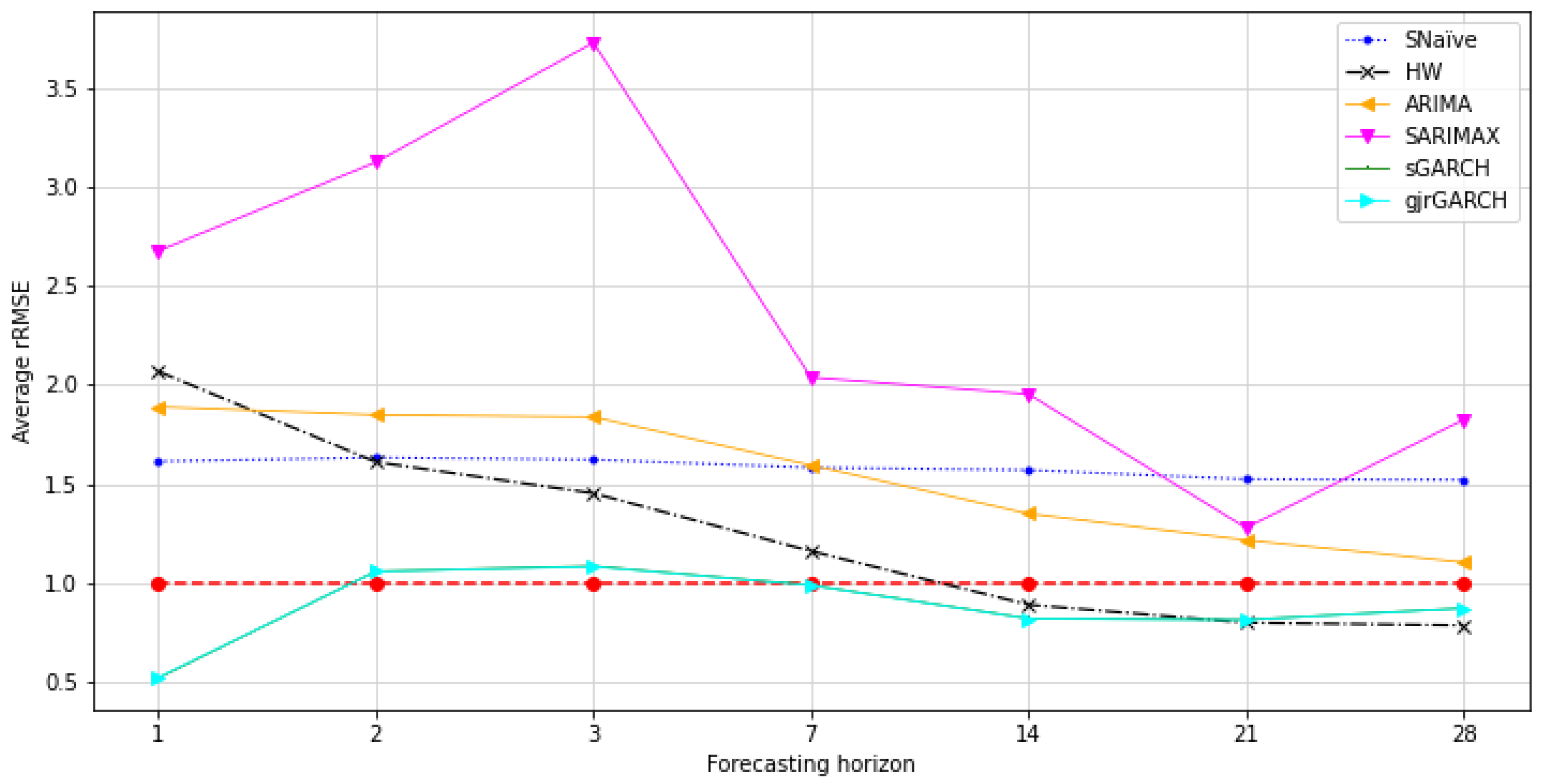
Similarly,

Table 4. Average rRMSE of forecasting methods.

Forecasting Methods	h = 1	h = 2	h = 3	h = 7	h = 14	h = 21	h = 28
Seasonal Naïve	1.613 **${}^{,•}$	1.633 *	1.622 **${}^{,•}$	1.582 **${}^{,‡}$	1.570 ***${}^{,†}$	1.523 ***${}^{,†}$	1.520
HW	2.069	1.610 *	1.452 **${}^{,†}$	1.159 ***${}^{,‡}$	0.888	0.797 ***${}^{,†}$	0.783 ***${}^{,†}$
ARIMA	1.890	1.849 *	1.838 ***${}^{,†}$	1.594	1.349	1.215 ***${}^{,†}$	1.103
SARIMAX	2.679 **${}^{,•}$	3.128 **${}^{,•}$	3.733 ***${}^{,†}$	2.039 ***${}^{,†}$	1.954	1.277 ***${}^{,†}$	1.824
sGARCH-sttd	0.517 *	1.057 **${}^{,•}$	1.083 ***${}^{,†}$	0.987 ***${}^{,†}$	0.818	0.812 ***${}^{,†}$	0.870 ${}^{†}$
gjrGARCH-sged	0.520 *	1.056 **${}^{,•}$	1.081 ***${}^{,†}$	0.986 ***${}^{,†}$	0.817	0.811 ***${}^{,†}$	0.869 ***
ANN-MLP	1.000	1.000	1.000	1.000	1.000	1.000	1.000

Note: statistically significant difference between the ANN-MLP forecast and the various forecast models based on the DM test at * p = 0.10, ** p = 0.05, and *** p = 0.01. A statistically significant difference between the distribution of forecasts based on the HLN test at ${}^{•}$ p = 0.10, ${}^{‡}$ p = 0.05, and ${}^{†}$ p = 0.01.

provides an additional comparison of relative accuracy measures of horizons 1 to 28 ahead forecast by the forecasting method according to rRMSE. We assess the out-of-sample forecasts for statistically significant differences using the DM and HLN tests. Figure 6 shows the relevant out-of-sample accuracy while a narrow examination makes it clear that the ANN-MLP forecast based on the raw data outperforms the other models, between horizon 2 to 7, except for the GARCH models for h = 1 and GARCH models for horizons 7 to 28 and the Holt–Winters method for horizons 14, 21, and 28, which are more accurate.

4. Conclusions

In this study, we have examined various forecasting methods for hotel demand. We introduced a framework and its application to estimate the hotel demand based on daily disaggregate data and numerous exogenous variables. Forecasting accuracy is regarded as a significant determinant of the revenue manager’s daily work to revenue maximization. Therefore, it is vital to identify a model which might generate more robust estimation accuracy that is easily applicable. In this study, using empirical results, we examine if the results will indicate more robust predictions for different models, including a SARIMAX model with exogenous variables compared to ANN-MLP and the other statistical models. Moreover, we incorporated symmetric and asymmetric conditional volatility models, GARCH and GJR-GARCH. Following the literature, neural network models tend to outperform forecasts from other forecasting models [45]. To measure the performance achieved by ANN-MLP, we have indicated ANN-MLP as the benchmark model for all evaluations.

Observations from the relative mean absolute percentage error (rMAPE) revealed that SARIMAX outperformed the various models in every seven forecast horizons except for the one-step horizon (h = 1), where ANN generated more robust results. In addition, the GARCH-sttd and GJR-GARCH-sged models showed significant evidence of effectiveness when seeking to forecast daily hotel demand. The empirical results indicated that the models were able to outperform every other one. Specifically, the findings reveal significant gains in accuracy levels when examining the daily demand time series. This confirms the work by Divino and McAleer (2010) [38]. We also found that the Holt–Winters and the ARIMA method perform best in four out of seven horizon periods (horizon: seven to 28), verifying that simple techniques can outperform more advanced [26]. Our results are in line with the study of [4], who indicated that each forecasting method demonstrates drawbacks in addition to the market challenges, the forecasting horizon, and the level of accuracy uncertainty [5].

Finally, hotel demand exhibits several seasonal effects with weekly patterns (intra-week and weekend patterns) with a seven-day, low, medium, and high seasonal pattern with an annual seasonal pattern. Therefore, considering that hotel demand exhibits high trends and seasonal patterns influenced by external factors that impact the performance, this study’s results provide a valuable tool for revenue managers. Therefore, we believe that the empirical results of the SARIMAX, including exogenous factors such as temperature, holidays, competitive set rank, and weekday, or the GARCH models create an enormous potential framework to support revenue management decisions.

The hotel demand market shows substantial volatility daily due to various events; thus, the current study is based on the specific hotel data and location. Hence, using a different dataset and location might boost the model’s performance and provide more accurate estimations. Further work might develop different results by using the same or other forecasting techniques. In addition, the exogenous variables used in the study impact the forecasting accuracy. While some broad qualitative conclusions about the importance of various features and the use of SARIMAX and ANN-MLP in daily demand observations can be drawn from our results, the particular choice of exogenous variables, etc. may not be universally applicable across other studies. Similarly, we might control the number of outliers more efficiently while understanding machine learning algorithms’ limits.

References

- Pan, B.; Yang, Y. Forecasting destination weekly hotel occupancy with big data. J. Travel Res. 2017, 56, 957–970. [Google Scholar] [CrossRef] [Green Version]
- Schwartz, Z.; Uysal, M.; Webb, T.; Altin, M. Hotel daily occupancy forecasting with competitive sets: A recursive algorithm. Int. J. Contemp. Hosp. Manag. 2016, 28, 267–285. [Google Scholar] [CrossRef]
- Pereira, L.N. An introduction to helpful forecasting methods for hotel revenue management. Int. J. Hosp. Manag. 2016, 58, 13–23. [Google Scholar] [CrossRef]
- Van Ryzin, G.J. Future of revenue management: Models of demand. J. Revenue Pricing Manag. 2005, 4, 204–210. [Google Scholar] [CrossRef]
- Oh, C.O.; Morzuch, B.J. Evaluating time-series models to forecast the demand for tourism in Singapore: Comparing within-sample and postsample results. J. Travel Res. 2005, 43, 404–413. [Google Scholar] [CrossRef]
- Witt, S.F.; Witt, C.A. Modeling and Forecasting Demand in Tourism; Academic Press Ltd.: Cambridge, MA, USA, 1992. [Google Scholar]
- Crouch, G.I. The study of international tourism demand: A review of findings. J. Travel Res. 1994, 33, 12–23. [Google Scholar] [CrossRef]
- Law, R. Initially testing an improved extrapolative hotel room occupancy rate forecasting technique. J. Travel Tour. Mark. 2004, 16, 71–77. [Google Scholar] [CrossRef]
- Schwartz, Z.; Cohen, E. Hotel revenue-management forecasting: Evidence of expert-judgment bias. Cornell Hotel Restaur. Adm. Q. 2004, 45, 85–98. [Google Scholar] [CrossRef]
- Li, G.; Song, H.; Witt, S.F. Recent developments in econometric modeling and forecasting. J. Travel Res. 2005, 44, 82–99. [Google Scholar] [CrossRef] [Green Version]
- Wong, K.K.; Song, H.; Chon, K.S. Bayesian models for tourism demand forecasting. Tour. Manag. 2006, 27, 773–780. [Google Scholar] [CrossRef] [Green Version]
- Song, H.; Li, G.; Witt, S.F.; Fei, B. Tourism demand modelling and forecasting: How should demand be measured? Tour. Econ. 2010, 16, 63–81. [Google Scholar] [CrossRef] [Green Version]
- Haensel, A.; Koole, G. Booking horizon forecasting with dynamic updating: A case study of hotel reservation data. Int. J. Forecast. 2011, 27, 942–960. [Google Scholar] [CrossRef]
- Song, H.; Smeral, E.; Li, G.; Chen, J. Tourism forecasting using econometric models. In Trends in European Tourism Planning and Organisation; Costa, C., Panyik, E., Buhalis, D., Eds.; Channel View: Bristol, UK, 2013; pp. 289–309. [Google Scholar]
- Ampountolas, A. Forecasting hotel demand uncertainty using time series Bayesian VAR models. Tour. Econ. 2018, 25, 734–756. [Google Scholar] [CrossRef]
- Ampountolas, A.; Legg, M.P. A segmented machine learning modeling approach of social media for predicting occupancy. Int. J. Contemp. Hosp. Manag. 2021, 33, 2001–2021. [Google Scholar] [CrossRef]
- Shen, H.; Huang, J.Z. Forecasting Time Series of Inhomogeneous Poisson Processes with Application to Call Center Workforce Management. Ann. Appl. Stat. 2008, 2, 601–623. [Google Scholar] [CrossRef]
- Barrow, D.; Kourentzes, N. The impact of special days in call arrivals forecasting: A neural network approach to modelling special days. Eur. J. Oper. Res. 2018, 264, 967–977. [Google Scholar] [CrossRef] [Green Version]
- De Livera, A.M.; Hyndman, R.J.; Snyder, R.D. Forecasting time series with complex seasonal patterns using exponential smoothing. J. Am. Stat. Assoc. 2011, 106, 1513–1527. [Google Scholar] [CrossRef] [Green Version]
- Glosten, L.R.; Jagannathan, R.; Runkle, D.E. On the relation between the expected value and the volatility of the nominal excess return on stocks. J. Financ. 1993, 48, 1779–1801. [Google Scholar] [CrossRef]
- Diebold, F.X.; Mariano, R.S. Comparing predictive accuracy. J. Bus. Econ. Stat. 1995, 13, 253–263. [Google Scholar]
- Harvey, D.; Leybourne, S.; Newbold, P. Testing the equality of prediction mean squared errors. Int. J. Forecast. 1997, 13, 281–291. [Google Scholar] [CrossRef]
- Box, G.E.; Jenkins, G.M. Time series analysis: Forecasting and control. In Holden-Day Series in Time Series Analysis; Holden-Day: Hoboken, NJ, USA, 1976. [Google Scholar]
- Hyndman, R.J.; Athanasopoulos, G. Forecasting: Principles and Practice; OTexts: Melbourne, Australia, 2018. [Google Scholar]
- Hyndman, R.; Koehler, A.B.; Ord, J.K.; Snyder, R.D. Forecasting with Exponential Smoothing: The State Space Approach; Springer Science & Business Media: Berlin/Heidelberg, Germany, 2008. [Google Scholar]
- Taylor, J.W. Triple seasonal methods for short-term electricity demand forecasting. Eur. J. Oper. Res. 2010, 204, 139–152. [Google Scholar] [CrossRef] [Green Version]
- Hyndman, R.J. Forecasting with Long Seasonal Periods. 2010. Available online: https://robjhyndman.com/hyndsight/longseasonality/ (accessed on 12 September 2019).
- Makridakis, S.; Wheelwright, S.; McGee, V. Forecasting: Methods and Applications, 2nd ed.; Wiley: Hoboken, NJ, USA, 1983. [Google Scholar]
- Dickey, D.A.; Fuller, W.A. Distribution of the Estimators for Autoregressive Time Series With a Unit Root. J. Am. Stat. Assoc. 1979, 74, 427–431. [Google Scholar]
- Hyndman, R.; Khandakar, Y. Automatic Time Series Forecasting: The forecast Package for R. J. Stat. Softw. Artic. 2008, 27, 1–22. [Google Scholar] [CrossRef] [Green Version]
- Osborn, D.R.; Chui, A.P.; Smith, J.P.; Birchenhall, C.R. Seasonality and the order of integration for consumption. Oxf. Bull. Econ. Stat. 1988, 50, 361–377. [Google Scholar] [CrossRef]
- Shapiro, S.S.; Wilk, M.B. An analysis of variance test for normality (complete samples). Biometrika 1965, 52, 591–611. [Google Scholar] [CrossRef]
- Zhang, G.; Patuwo, B.E.; Hu, M.Y. Forecasting with artificial neural networks:: The state of the art. Int. J. Forecast. 1998, 14, 35–62. [Google Scholar] [CrossRef]
- Law, R. Room occupancy rate forecasting: A neural network approach. Int. J. Contemp. Hosp. Manag. 1998, 10, 234–239. [Google Scholar] [CrossRef]
- Wu, D.C.; Song, H.; Shen, S. New developments in tourism and hotel demand modeling and forecasting. Int. J. Contemp. Hosp. Manag. 2017, 29, 507–529. [Google Scholar] [CrossRef]
- Engle, R.F. Autoregressive conditional heteroscedasticity with estimates of the variance of United Kingdom inflation. Econom. J. Econom. Soc. 1982, 50, 987–1007. [Google Scholar] [CrossRef]
- Bollerslev, T. Generalized autoregressive conditional heteroskedasticity. J. Econom. 1986, 31, 307–327. [Google Scholar] [CrossRef] [Green Version]
- Divino, J.A.; McAleer, M. Modelling and forecasting daily international mass tourism to Peru. Tour. Manag. 2010, 31, 846–854. [Google Scholar] [CrossRef]
- Chan, F.; Lim, C.; McAleer, M. Modelling multivariate international tourism demand and volatility. Tour. Manag. 2005, 26, 459–471. [Google Scholar] [CrossRef]
- Shareef, R.; McAleer, M. Modelling international tourism demand and uncertainty in Maldives and Seychelles: A portfolio approach. Math. Comput. Simul. 2008, 78, 459–468. [Google Scholar] [CrossRef] [Green Version]
- Liang, Y.H. Forecasting models for Taiwanese tourism demand after allowance for Mainland China tourists visiting Taiwan. Comput. Ind. Eng. 2014, 74, 111–119. [Google Scholar] [CrossRef]
- Hyndman, R.J.; Koehler, A.B. Another look at measures of forecast accuracy. Int. J. Forecast. 2006, 22, 679–688. [Google Scholar] [CrossRef] [Green Version]
- Lin, H.L.; Liu, L.M.; Tseng, Y.H.; Su, Y.W. Taiwan’s international tourism: A time series analysis with calendar effects and joint outlier adjustments. Int. J. Tour. Res. 2011, 13, 1–16. [Google Scholar] [CrossRef]
- Chen, C.; Liu, L.M. Joint estimation of model parameters and outlier effects in time series. J. Am. Stat. Assoc. 1993, 88, 284–297. [Google Scholar]
- Claveria, O.; Monte, E.; Torra, S. A new forecasting approach for the hospitality industry. Int. J. Contemp. Hosp. Manag. 2015, 27, 1520–1538. [Google Scholar] [CrossRef] [Green Version]
Figure 1.
Daily totals for demand and temperature.
Figure 2.
Hotel daily total demand.
Figure 3.
Day of the week demand for the entire data set.
Figure 4.
Dataset variables’ correlation.
Figure 5.
Average rMAPE of forecasting methods.
Figure 6.
Average rRMSE of Forecasting Methods.