On the Autoregressive Time Series Model Using Real and Complex Analysis

Abstract

The autoregressive model is a tool used in time series analysis to describe and model time series data. Its main structure is a linear equation using the previous values to compute the next time step; i.e., the short time relationship is the core component of the autoregressive model. Therefore, short-term effects can be modeled in an easy way, but the global structure of the model is not obvious. However, this global structure is a crucial aid in the model selection process in data analysis. If the global properties are not reflected in the data, a corresponding model is not compatible. This helpful knowledge avoids unsuccessful modeling attempts. This article analyzes the global structure of the autoregressive model through the derivation of a closed form. In detail, the closed form of an autoregressive model consists of the basis functions of a fundamental system of an ordinary differential equation with constant coefficients; i.e., it consists of a combination of polynomial factors with sinusoidal, cosinusoidal, and exponential functions. This new insight supports the model selection process.

1. Introduction

The increasing digitalization of all areas of society and the economy is leading to ever greater volumes of data. Many of these data are time series; i.e., they have a time component by which they can be ordered. When analyzing time series—with the aim of predicting future values or gaining knowledge about the underlying, generating process—mathematical model building plays a crucial role.

In general, two types of models can be distinguished: domain-specific models on the one hand and general-purpose models on the other. As a rule of thumb, domain-specific models are preferable for corresponding (domain) problems. This rule corresponds to the principle of using existing knowledge, especially if this information is already reflected in the mathematical model. For example, when modeling radioactive decay [1] or the endemic development of a pandemic [2], a domain-specific model is a good starting point for data analysis. If this background knowledge about the domain and the use-case is not available or if this knowledge should not be used, general purpose models can be used for prediction. Many of these general purpose models exist and are explained in standard textbooks [3].

In mathematical modeling and model building, it is important that essential properties of a model are reflected in the data. If the data contradict the character of a model, the quality of the model-based prediction suffers; e.g., if the model has a linear relationship, although the data rather correspond to a parabola, a contradiction is given and the model is at most to be used with caution or is to be rejected. However, this decision assumes that all essential characteristics of a model are known and are not a black box. It is in this context that this article should be seen: the following sections describe the autoregressive model for time series. The characteristics of the model are usually interpreted using stochastic model building; this article shows a novel, different, analytical approach through the derivation of a closed form and thus reveals additional important model properties. In detail, the closed form of an autoregressive model consists of a combination of polynomial factors with sinusoidal, cosinusoidal, and exponential functions. This new insight supports the model selection process.

2. Related Work: The Autoregressive Model

Definition 1.

A time series is a sequence of pairs $(x_i,y_i)$ that consist of a time component $x_i$ and an arbitrary component $y_i$. To allow for the possibly unpredictable nature of future observations, it is natural to suppose that each observation is a realized value of a certain random variable [4]. The time component can be continuous $x_i\in \mathbb{R}$ or discrete $x_i\in \mathbb{Z}$. If the context describes the timing implicitly—e.g., by a regular sampling in fixed intervals—the time component may be omitted.

The distinction between discreteness and continuity can be approached in various ways. John L. Bell explains “To be continuous is to constitute an unbroken or uninterrupted whole, like the ocean or the sky. A continuous entity—a continuum—has no `gaps’. Opposed to continuity is discreteness: to be discrete is to be separated, like the scattered pebbles on a beach or the leaves on a tree. Continuity connotes unity; discreteness, plurality” [5]. In addition to mathematical definitions and philosophical considerations [6], applied mathematics adds a pragmatic perspective: in many cases, organizational, practical, or technical conditions determine whether a variable can be considered discrete or continuous. This article does not make a strict distinction between continuous and discrete, but uses both interpretations in parallel.

In order to capture and analyze a time series mathematically, a mathematical model is required. A time series model for the observed data is a specification of the joint distributions of a sequence of random variables [4]. This article refers exclusively to the autoregressive (AR) model. According to Judy L. Klein, the AR-model originated in the 1920s and was first applied by Udny Yule in his 1927 analysis of the time-series behavior of sunspots [7].

Definition 2.

The autoregressive model AR$\left(p\right)$ determines the value of a process at an arbitrary time step t using a linear combination of the p-last values:

$$y_t={\varphi }_1·y_{t-1}+{\varphi }_2·y_{t-2}+\dots +{\varphi }_p·y_{t-p}+{\epsilon }_t$$

(1)

The number p is called the order of the AR model.The weights ${\varphi }_i$ of the linear combination are the model parameters. They are considered to be constant. Furthermore, an AR model assumes that this process is superimposed by white noise; i.e. the ${\epsilon }_t$ are assumed to be uncorrelated with each other in time and identically distributed, with an expected value of zero and finite variance. This model is abbreviated as AR$\left(p\right)$.

Many definitions additionally require that the process described by AR $\left(p\right)$ is stationary. This results in further conditions on the coefficients ${\varphi }_i$, which are not a focus of the following considerations of this article.

The application of the AR$\left(p\right)$ model to describe a given time series

$$\dots ,y_{t-3},y_{t-2},y_{t-1},y_t,y_{t+1},y_{t+2},y_{t+3},\dots$$

(2)

raises several questions. Two of these questions concern the global structure of the model:

• Is the AR$\left(p\right)$ model in principle able to describe characteristic properties of the time series (2); in other words, is the AR$\left(p\right)$ model in principle suitable?
• If it is suitable, how is the parameter p selected?

Stating these questions in other words, what is the closed form of the model?

The model and its parameters are usually determined using a stochastic/statistical perspective [8,9]: the commonly used approaches are based on maximizing a likelihood function and obtaining the model parameters via the solution of the so-called modified Yule–Walker equations [10] or via ordinary least squares regression [11].

This article does not provide a new approach to select an appropriate model or to determine the model parameters; this article concentrates on the question of the closed form of the model. The goal is to derive an expression that can be used to evaluate any time step t without having to evaluate all previous values first. This approach to the AR model explicitly names the elementary building blocks of the model. These elementary building blocks should be reflected in the data—an insight that contributes to model selection and that gives decision support during the model building process. The only existing approach to the global structure of the autoregressive model has been presented by Dihui Lai and Bingfeng Lu: in “Understanding Autoregressive Model for Time Series as a Deterministic Dynamic System” [12], they interpret a first-order difference equation as an autoregressive model $y_t={\varphi }_0+{\varphi }_1{y}_{t-1}$. The assumed change over time in this formula is one unit. In general, the time step can be of any unit, and by changing the unit of time, it can be replaced with $\Delta t$, and the equation can be rewritten as

$$\frac{y_t-y_{t\mathsf{-}\Delta t}}{\Delta t}={\varphi }_0+({\varphi }_1-1)y_{t-\mathsf{\Delta }t}.$$

(3)

In the limit case $\Delta t\to 0$, the difference equation becomes a first-order time-dependent ordinary differential equation (ODE):

$$\frac{\mathrm{d}y}{\mathrm{d}t}={\varphi }_0+({\varphi }_1-1)y.$$

(4)

3. Global Structure

This article extends the state-of-the-art using eigenanalysis and ordinary differential equations in order to reveal important global properties of the AR$\left(p\right)$ model, which should be reflected in the time series data and which provide decision support when selecting the model to describe a time series.

3.1. Eigenanalysis

The AR$\left(p\right)$ model can be interpreted as a linear operator applied to an initial vector consisting of the data of the time series. The equation of the definition (1) is formulated in this interpretation as a matrix equation

$$\underset{={\mathbf{y}}_t}{\underbrace{\left(\begin{array}{c}{y}_t\\ y_{t-1}\\ ⋮\\ y_{t-p+1}\end{array}\right)}}={\mathbf{A}}_p·\left(\begin{array}{c}{y}_{t-1}\\ y_{t-2}\\ ⋮\\ y_{t-p}\end{array}\right)$$

(5)

with a matrix

$${\mathbf{A}}_p=\left(\begin{array}{ccccccc}{\varphi }_1& {\varphi }_2& {\varphi }_3& \dots & {\varphi }_{p-2}& {\varphi }_{p-1}& {\varphi }_p\\ 1& 0& 0& \dots & 0& 0& 0\\ 0& 1& 0& \dots & 0& 0& 0\\ ⋮& \ddots & \ddots & \ddots & \ddots & \ddots & ⋮\\ 0& \dots & 0& 1& 0& 0& 0\\ 0& \dots & 0& 0& 1& 0& 0\\ 0& \dots & 0& 0& 0& 1& 0\end{array}\right)$$

(6)

containing the model parameters ${\varphi }_1$, …, ${\varphi }_p$. The forecast of the next k values is then simply the k-fold application of the linear operator ${\mathbf{A}}_p$:

$${\mathbf{y}}_{t+k}=\underset{={\mathbf{A}}_p^k}{\underbrace{{\mathbf{A}}_p·\dots \cdots {\mathbf{A}}_p}}·{\mathbf{y}}_t$$

(7)

This equation can be transformed into a closed form for model orders $p=1,\dots ,4$ via Jordan normal form [13]. For this purpose, the roots of the characteristic polynomial of the matrix ${\mathbf{A}}_p$ and the corresponding eigenvectors have to be determined. For the characteristic polynomial, the following applies:

Theorem 1.

The characteristic polynomial of ${\mathbf{A}}_p$ is

$${\chi }_p\left(\lambda \right)={(-1)}^p·({\lambda }^p-{\varphi }_1{\lambda }^{p-1}-\dots -{\varphi }_{p-1}\lambda -{\varphi }_p).$$

(8)

Proof. 

The case $p=1$ with

$$\begin{array}{cc}\hfill det({\mathbf{A}}_1-\lambda \mathbf{I})& =det({\varphi }_1-\lambda )={\varphi }_1-\lambda \hfill \end{array}$$

(9)

$$\begin{array}{cc}\hfill & =-1·(\lambda -{\varphi }_1)={\chi }_1\left(\lambda \right)\hfill \end{array}$$

(10)

is the base case of an induction. The induction step starts with

$$\begin{array}{cc}\hfill det({\mathbf{A}}_p-\lambda \mathbf{I})& =det\left(\begin{array}{ccccccc}{\varphi }_1-\lambda & {\varphi }_2& {\varphi }_3& \dots & {\varphi }_{p-2}& {\varphi }_{p-1}& {\varphi }_p\\ 1& -\lambda & 0& \dots & 0& 0& 0\\ 0& 1& -\lambda & \dots & 0& 0& 0\\ ⋮& \ddots & \ddots & \ddots & \ddots & \ddots & ⋮\\ 0& \dots & 0& 1& -\lambda & 0& 0\\ 0& \dots & 0& 0& 1& -\lambda & 0\\ 0& \dots & 0& 0& 0& 1& -\lambda \end{array}\right)\hfill \end{array}$$

and the determinant of this matrix will be computed by using the Laplace expansion along its last column.

$$\begin{array}{cc}\hfill det({\mathbf{A}}_p-\lambda \mathbf{I})& =-{(-1)}^p·{\varphi }_p·det\left(\begin{array}{cccc}1& -\lambda & 0& \dots \\ 0& 1& -\lambda & \dots \\ ⋮& \ddots & \ddots & \ddots \\ 0& \dots & 0& 1\end{array}\right)\hfill \\ \hfill & +(-\lambda )·det({\mathbf{A}}_{p-1}-\lambda \mathbf{I})\hfill \end{array}$$

(11)

The Laplace expansion reduces the $p\times p$ matrix $({\mathbf{A}}_p-\lambda \mathbf{I})$ into two matrices. The determinate of the first matrix is one, since its structure contains a lower triangular matrix of zeros, and the product of the diagonal is one. The second matrix meets the induction hypothesis. As a consequence, due to

$$\begin{array}{cc}\hfill det({\mathbf{A}}_p-\lambda \mathbf{I})& ={(-1)}^p·(-{\varphi }_p)-\lambda ·det({\mathbf{A}}_{p-1}-\lambda \mathbf{I})\hfill \\ \hfill & ={(-1)}^p·(-{\varphi }_p)-\lambda ·\hfill \end{array}$$

(12)

$$\begin{array}{cc}\hfill & \left[{(-1)}^{p-1}·({\lambda }^{p-1}-{\varphi }_1{\lambda }^{p-2}-\dots -{\varphi }_{p-2}\lambda -{\varphi }_{p-1})\right]\hfill \end{array}$$

(13)

$$\begin{array}{cc}\hfill & ={(-1)}^p\left(-{\varphi }_p+\lambda ·({\lambda }^{p-1}-{\varphi }_1{\lambda }^{p-2}-\dots -{\varphi }_{p-2}\lambda -{\varphi }_{p-1})\right)\hfill \end{array}$$

(14)

$$\begin{array}{cc}\hfill & ={(-1)}^p\left({\lambda }^p-{\varphi }_1{\lambda }^{p-1}-\dots -{\varphi }_{p-2}{\lambda }^2-{\varphi }_{p-1}\lambda -{\varphi }_p\right)\hfill \end{array}$$

(15)

the characteristic polynomial of ${\mathbf{A}}_p$ is ${\chi }_p\left(\lambda \right)$. □

Having calculated the eigenvectors and the eigenspaces, the matrix ${\mathbf{A}}_p$ can be decomposed into ${\mathbf{A}}_p={\mathbf{T}}^{-1}\mathbf{D}\mathbf{T}$ with an orthogonal basis $\mathbf{T}$. The matrix $\mathbf{D}$ is a diagonal matrix, if and only if the sum of the dimensions of its eigenspaces is equal to p. Otherwise, it is almost diagonal; i.e., with only non-zero elements on its diagonal and ones on its superdiagonal. Consequently, the k-fold application of the linear operator ${\mathbf{A}}_p$ is

$$\begin{array}{cc}\hfill {\mathbf{A}}_p^k& ={\left(\mathbf{T}\mathbf{D}{\mathbf{T}}^{-1}\right)}^k\hfill \\ \hfill & =\mathbf{T}\mathbf{D}\underset{=\mathbf{I}}{\underbrace{{\mathbf{T}}^{-1}·\mathbf{T}}}\mathbf{D}{\mathbf{T}}^{-1}·\dots ·\mathbf{T}\mathbf{D}{\mathbf{T}}^{-1}\hfill \\ \hfill & =\mathbf{T}{\mathbf{D}}^k{\mathbf{T}}^{-1}.\hfill \end{array}$$

(16)

where ${\mathbf{D}}^k$ is usually easy to determine, meaning that Equation (7) can be evaluated to a closed form representation.

Example: The AR(2)-model (with $p=2$)

$$y_t=1·y_{t-1}+1·y_{t-2}\mathrm{with}{y}_0=0\mathrm{and}{y}_1=1$$

(17)

illustrates the previously presented approach. Written as linear operator, the AR(2)-model can be represented by the matrix

$${\mathbf{A}}_2=\left(\begin{array}{cc}1& 1\\ 1& 0\end{array}\right).$$

(18)

Hence, the characteristic polynomial is

$$\chi \left(\lambda \right)=det({\mathbf{A}}_2-\lambda \mathbf{I})={\lambda }^2-\lambda -1.$$

(19)

Its roots are ${\lambda }_{1/2}=\frac{1}{2}(1\pm \sqrt{5})$. Using the corresponding eigenvectors, the matrix ${\mathbf{A}}_2$ can be decomposed into

$${\mathbf{A}}_2=\mathbf{T}·\mathbf{D}·{\mathbf{T}}^{-1}$$

(20)

with

$$\mathbf{T}=\left(\begin{array}{cc}\frac{1}{2}-\frac{\sqrt{5}}{10}& \frac{1}{2}+\frac{\sqrt{5}}{10}\\ -\frac{\sqrt{5}}{5}& \frac{\sqrt{5}}{5}\end{array}\right)\mathrm{and}\mathbf{D}=\left(\begin{array}{cc}\frac{1}{2}-\frac{1}{2}\sqrt{5}& 0\\ 0& \frac{1}{2}+\frac{1}{2}\sqrt{5}\end{array}\right).$$

(21)

As a result, the closed form of this AR(2)-model is

$$\left(\begin{array}{c}{y}_{k+1}\\ y_k\end{array}\right)={\mathbf{A}}_2^k·\left(\begin{array}{c}{y}_1\\ y_0\end{array}\right)=\mathbf{T}·\left(\begin{array}{cc}{(\frac{1}{2}-\frac{1}{2}\sqrt{5})}^k& 0\\ 0& {(\frac{1}{2}+\frac{1}{2}\sqrt{5})}^k\end{array}\right)·{\mathbf{T}}^{-1}·\left(\begin{array}{c}{y}_1\\ y_0\end{array}\right),$$

(22)

respectively,

$$y_{k+1}=\left(\frac{1}{2}-\frac{3}{10}\sqrt{5}\right)·{\left(\frac{1}{2}-\frac{1}{2}\sqrt{5}\right)}^k+\left(\frac{1}{2}+\frac{3}{10}\sqrt{5}\right)·{\left(\frac{1}{2}+\frac{1}{2}\sqrt{5}\right)}^k,$$

(23)

which is equivalent to the well-known, closed formula to calculate the Fibonacci sequence.

This approach to derive a closed form equation can be used for model orders $p=1,\dots ,4$, but for higher-order models ($p>4$), the roots of the characteristic polynomial of the matrix ${\mathbf{A}}_p$ and the corresponding eigenvectors cannot be determined in general, although special cases may have an exact, analytic solution.

3.2. Differential Equations

A novel approach is based on the idea of Dihui Lai and Bingfeng Lu, summarized in Section 2: they interpret a first-order difference equation as an autoregressive model $y_t={\varphi }_0+{\varphi }_1{y}_{t-1}$. This idea is now extended towards higher order AR$\left(p\right)$ models. The basic idea of interpreting a difference equation as an AR model is symmetric; not only can the difference equation be interpreted as an AR model, but also vice versa. Furthermore, differential equations of higher degree correspond to AR models of higher order.

Besides the difference quotients in the following forms, namely forward difference

$$\frac{\Delta y}{\Delta t}=\frac{y_{t+\mathsf{\Delta }t}-y_t}{\Delta t},$$

(24)

backward difference

$$\frac{\Delta y}{\Delta t}=\frac{y_t-y_{t-\mathsf{\Delta }t}}{\Delta t},$$

(25)

and central difference

$$\frac{\Delta y}{\Delta t}=\frac{y_{t+\mathsf{\Delta }t}-y_{t-\mathsf{\Delta }t}}{2\Delta t},$$

(26)

to approximate the first-order derivative, there are also difference quotients for the numerical calculation of higher derivatives. The recursive definition of higher-order central difference quotients is

$$\frac{{\Delta }^{n}y}{\Delta t^n}=\frac{1}{\Delta t^n}·\sum _{k=0}^n{(-1)}^k\left(\genfrac{}{}{0pt}{}{n}{k}\right)y_{t+k-n/2}$$

(27)

for even degrees of n, and

$$\frac{{\Delta }^{n}y}{\Delta t^n}=\frac{1}{2\Delta t^n}·\sum _{k=0}^{n-1}{(-1)}^k\left(\genfrac{}{}{0pt}{}{n-1}{k}\right)·\left(y_{t+k+1-(n-1)/2}-y_{t+k-1-(n-1)/2}\right)$$

(28)

for odd degrees of n. In the limit analysis for $\Delta t\to 0$, the general AR$\left(p\right)$ model becomes an ODE of order $n=p$; i.e., Equation (1) becomes

$$a_n{y}^{\left(n\right)}+a_{n-1}{y}^{(n-1)}+\dots +a_2{y}^{″}+a_1{y}^{\prime }+a_{0}y=f\left(x\right)$$

(29)

with constants $a_i$, respectively, in normalized representation with $a_n=1$:

$$y^{\left(n\right)}+a_{n-1}{y}^{(n-1)}+\dots +a_2{y}^{″}+a_1{y}^{\prime }+a_{0}y=f\left(x\right).$$

(30)

The solution of this equation can be calculated with the help of the characteristic polynomial of the ODE [14], which is obtained by substituting the k-th derivative by ${\lambda }^k$:

$$\chi \left(\lambda \right)={\lambda }^n+a_{n-1}{\lambda }^{(n-1)}+\dots +a_2{\lambda }^2+a_1\lambda +a_0.$$

(31)

According to the fundamental theorem of algebra, a polynomial of degree n has exactly n roots, counting multiplicity. If all coefficients $a_i$ are real, the roots are real or occur in conjugate pairs. Each root corresponds to an independent solution, which together form the fundamental system that represents all solutions of the homogeneous ODE (with $f\left(x\right)=0$). The necessary n linearly independent solutions can then be found using the rules to solve higher-order differential equations with constant coefficients:

If r is a real root that appears k times, then the solutions are

$$y=e^{r·t},y=t·e^{r·t},y=t^2·e^{r·t},\dots ,y=t^{k-1}·e^{r·t}.$$

(32)

If $r=\alpha \pm \beta i$ are complex conjugate roots appearing k times, then the solutions are

$$e^{\alpha ·t}cos(\beta ·t),e^{\alpha ·t}sin(\beta ·t),$$

(33)

$$t·e^{\alpha ·t}cos(\beta ·t),t·e^{\alpha ·t}sin(\beta ·t),$$

(34)

$$t^2·e^{\alpha ·t}cos(\beta ·t),t^2·e^{\alpha ·t}sin(\beta ·t),$$

(35)

$$⋮$$

$$t^{k-1}·e^{\alpha ·t}cos(\beta ·t),t^{k-1}·e^{\alpha ·t}sin(\beta ·t).$$

(36)

These building blocks of the fundamental system of the ODE are the components that compose the AR(p)-Model.

To illustrate these building blocks, the following synthetic example transforms an autoregressive model into a closed form representation. This is not the classical procedure in time series analysis. Time series analysis is usually a data-driven, inverse process; i.e., the time series are based on the assumption that there is a generating, stochastic process that is to be determined inversely from the data. In the following, synthetic example, we start from an exactly specified model, determine the time series realization from it, and determine the closed form. The last transformation step is in particular focus here—it shall clarify the connection between the representation according to Definition 2 (see Equation (1)) and the fundamental system in order to provide a more profound, theoretical insight. For practical applications, this approach is not recommended.

Example: An exemplary AR model shall consist of the initial values

$$y_0=1,y_{-1}=2,y_{-2}=0,$$

and an order $p=3$ linear combination with the coefficients 2, $-{}^3/{}_2$, and $-{}^1/{}_2$; i.e.,

$$y_t=2·y_{t-1}-\frac{3}{2}·y_{t-2}-\frac{1}{2}·y_{t-3}.$$

(37)

So-called white noise ${\epsilon }_i$ is not used in this example. For practical applications, this assumption is very problematic and should not be used; however, in this synthetic theoretical example, this assumption is used to illustrate the similarity of the two AR model representations: without white noise, numerical inaccuracies are the only deviations that may occur between the two representations.

This example model generates the sequence

$$\begin{array}{ccccc}{y}_{-2}=0.0\hfill & & y_{-1}=2.0\hfill & & y_0=1.0\hfill \\ y_1=-1.0\hfill & & y_2=-4.5\hfill & & y_3=-8.0\hfill \\ y_4=-8.75\hfill & & y_5=-3.25\hfill & & y_6=10.625\hfill \\ y_7=30.5\hfill & & y_8=46.6875\hfill & & y_9=42.3125\hfill \\ y_{10}=-0.65625\hfill & & y_{11}=-88.125\hfill & & y_{12}=-196.421875\hfill \\ ⋮\hfill \end{array}$$

As the AR(3)-model has an order of $p=3$, the corresponding ODE has a characteristic polynomial of degree three. Such a polynomial may take the following forms:

• Three real roots (counting multiplicity); or
• One real root and a conjugate pair.

In the first case, the fundamental system would consist of three exponential functions with polynomial factors up to degree two. This basis would not be able to produce the generated data sequence of the time series—in particular, several sign changes contradict this model.

In the second case, the fundamental system consists of an exponential function and a pair of exponential functions multiplied with sine/cosine factors. These basis functions are reflected in the data sequence: the trigonometric functions are responsible for the sign changes. As a consequence, this case applies; i.e., the characteristic polynomial has one real and two conjugate complex zeros. The starting point for the fundamental system is therefore

$$\begin{array}{cc}\hfill y& =a_0{e}^{a_1·x}\hfill \\ \hfill & +b_0{e}^{b_1·x}sin(b_2·x)+b_3{e}^{b_1·x}cos(b_2·x).\hfill \end{array}$$

(38)

This basis, together with the values of the AR model sequence,

$$\begin{array}{c}\hfill \begin{array}{ccccccc}0.0,& 2.0,& 1.0,& -1.0,& -4.5,& -8.0,& -8.75,\\ -3.25,& 10.625,& 30.5,& 46.6875,& 42.3125,& \dots \end{array}\end{array}$$

leads to an overdetermined, nonlinear system of equations, which can be solved with a numerical minimization procedure [15]. This optimization determines the fundamental system and simultaneously solves the initial value problem of the ODE:

$$\begin{array}{cccc}\hfill & a_0=-2.015059\mathrm{E}-12,\hfill & \hfill & a_1=-13.601814,\hfill \\ \hfill & b_0=2.5104196,\hfill & \hfill & b_1=0.35838324,\hfill \\ \hfill & b_2=11.896794,\hfill & \hfill & b_3=1.0790480.\hfill \end{array}$$

(39)

Using these constants in Equation (38) leads to a global description of the discrete model. In detail, the AR model

$$y_t=2·y_{t-1}-\frac{3}{2}·y_{t-2}-\frac{1}{2}·y_{t-3}$$

(40)

with the initial values $y_0=1,y_{-1}=2,y_{-2}=0$ can be represented by the closed form

$$\begin{array}{cc}\hfill y\left(x\right)& =-2.015059\mathrm{E}-12e^{-13.601814·x}\hfill \\ \hfill & +2.5104196e^{0.35838324·x}sin(11.896794·x)\hfill \\ \hfill & +1.0790480e^{0.35838324·x}cos(11.896794·x).\hfill \end{array}$$

(41)

The differences between both representations—the AR model and the ODE solution—if evaluated at discrete time stamps, are listed in

Table 1. The example AR model has lead to an ordinary differential equation whose solution is a fundamental system (38) with an initial value problem. The solution to the initial value problem (39) describes the AR model globally; i.e., the AR model consists of oscillating exponential terms. The small differences $\Delta$ between both representations are listed in the last column.

t,	Autoregressive Model	Fundamental System	Difference
Resp. x	${\mathit{y}}_{\mathit{t}}=2{\mathit{y}}_{\mathit{t}-1}-\frac{3}{2}{\mathit{y}}_{\mathit{t}-2}-\frac{1}{2}{\mathit{y}}_{\mathit{t}-3}$	$\mathit{y}\left(\mathit{x}\right)={\mathit{a}}_0{\mathit{e}}^{{\mathit{a}}_1\mathit{x}}+{\mathit{b}}_0{\mathit{e}}^{{\mathit{b}}_1\mathit{x}}sin\left({\mathit{b}}_2\mathit{x}\right)$	$\Delta$
		$+{\mathit{b}}_3{\mathit{e}}^{{\mathit{b}}_1\mathit{x}}cos\left({\mathit{b}}_2\mathit{x}\right)$
0	1.0000000	1.0790479	0.0790479
1	−1.0000000	−1.0189353	0.0189353
2	−4.5000000	−4.4962394	0.0037605
3	−8.0000000	−8.0033071	0.0033071
4	−8.7500000	−8.7525921	0.0025921
5	−3.2500000	−3.2522651	0.0022651
6	10.6250000	10.6252496	0.0002496
7	30.5000000	30.5038138	0.0038138
8	46.6875000	46.6943506	0.0068506
9	42.3125000	42.3197350	0.0072350
10	−0.6562500	−0.6522115	0.0040384
11	−88.1250000	−88.1260007	0.0010007
12	−196.4218750	−196.4254673	0.0035923
13	−260.3281250	−260.3283357	0.0002107
14	−181.9609375	−181.9552121	0.0057253
15	124.7812500	124.7800496	0.0012003

. Small differences are shown, which were to be expected in the range of numerical inaccuracies of floating point arithmetic.

The approach of interpreting an arbitrary AR(p) model as a differential equation is new and allows the identification of the global structure: the building blocks of the fundamental system of the corresponding ordinary differential equation are the components of which the AR(p) model consists. The last example has illustrated this approach explicitly. Furthermore, the first example using the Fibonacci sequence (17) can be interpreted in this way and leads to an equivalent solution:

Example: The Fibonacci sequence (17) has the closed form

$$y_{k+1}=\left(\frac{1}{2}-\frac{3}{10}\sqrt{5}\right)·{\left(\frac{1}{2}-\frac{1}{2}\sqrt{5}\right)}^k+\left(\frac{1}{2}+\frac{3}{10}\sqrt{5}\right)·{\left(\frac{1}{2}+\frac{1}{2}\sqrt{5}\right)}^k,$$

(42)

To outline its structure, this formula can be rewritten in terms of exponential functions

$$y_{k+1}=\left(\frac{1}{2}-\frac{3}{10}\sqrt{5}\right)·{\mathbf{e}}^{k·ln\left(\frac{1}{2}-\frac{1}{2}\sqrt{5}\right)}+\left(\frac{1}{2}+\frac{3}{10}\sqrt{5}\right)·{\mathbf{e}}^{k·ln\left(\frac{1}{2}+\frac{1}{2}\sqrt{5}\right)},$$

(43)

This representation shows that the Fibonacci sequence is essentially composed of two exponential functions that dominate the trend of the corresponding time series. This is consistent with the global structure resulting from the fundamental system of the ODE as derived in this article: an AR(2) model leads to a differential equation of degree two; the corresponding characteristic polynomial of the ODE therefore also has degree two and thus has either two real roots (counting multiplicity) or two conjugate complex roots. The second case can be excluded, since this case would lead to trigonometric factors and thus to sign changes in the data series. The first case with two real zeros, on the other hand, leads exactly to the two exponential functions, which overlap as in Equation (43).

4. Application

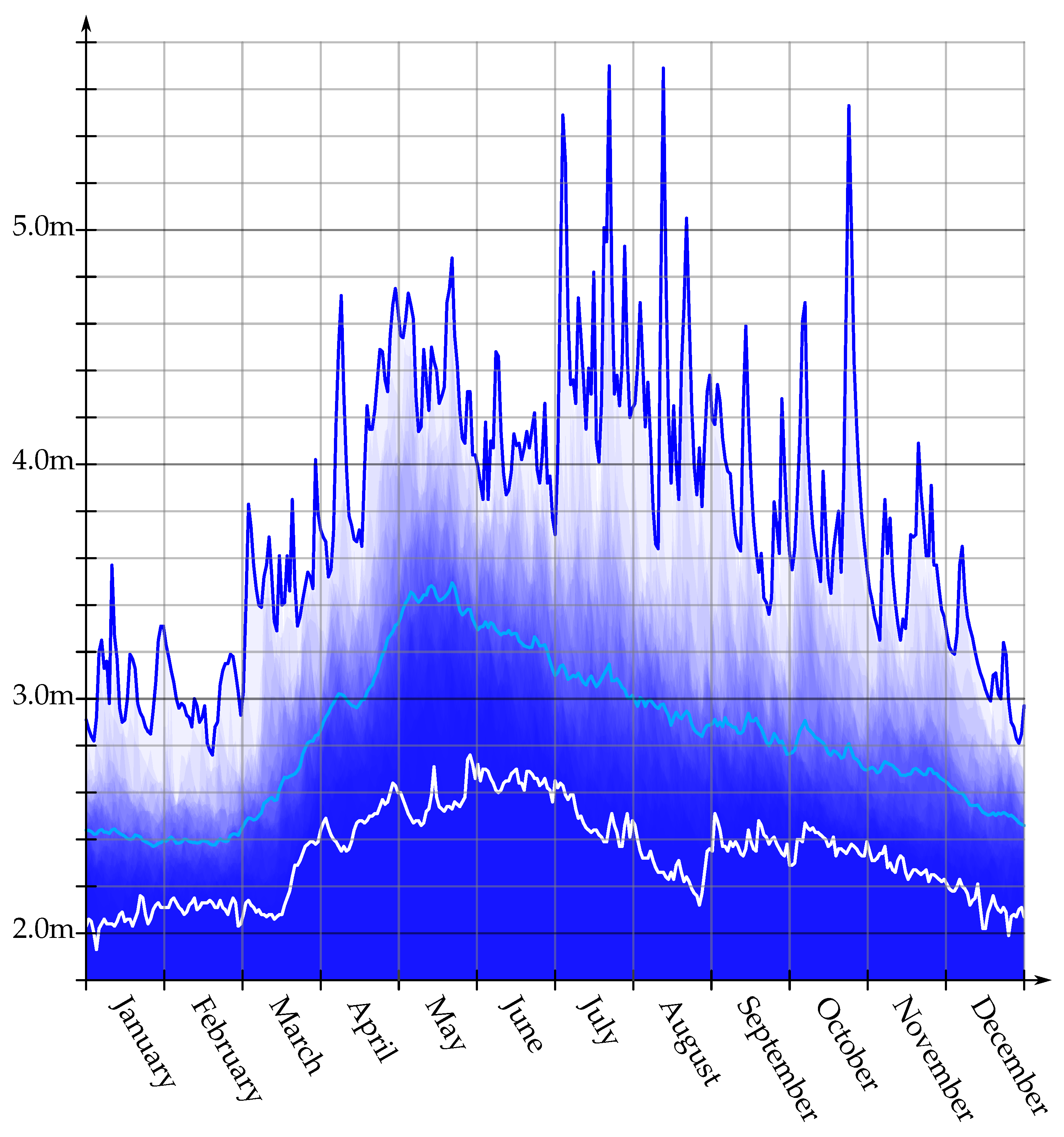
In order to illustrate the application of the gained knowledge about the global structure, an example data set is used: the data set is the level of the river Mur measured by the Graz station, Austria (DBMS #6001082), as provided by the web-service https://ehyd.gv.at (accessed 15 May 2020). The data set consists of one measurement of the water level per day starting on 1 January 1976 and running until 31 December 2016. A visual overview is shown in Figure 1. The diagram shows the annual data. Each year is plotted using a semi-transparent, blue-filled area plot on top of each other. Additionally, the diagram contains, for each day of a year, the minimum (white), average (light blue), and maximum (dark blue) water levels of all years (1976–2016) on the corresponding day. These values are visualized in line plots.

In this example, the goal is to forecast the water levels of the next three days on the basis of the previous 50 days; i.e., starting with 1 January 1976, a sliding window of 50 days is used to determine an autoregressive model of order three (AR(3)) in order to forecast the water level of the next three days. In detail, the test consists of 14,974 time series of 50 values each with the challenge to predict the next three values. As the historic data are complete, the quality of the forecast can be evaluated using the ground truth.

This test is performed with two algorithmic approaches. The first approach determines the parameters of the AR(3) model via ordinary least squares regression as described by M. Hauser, [11]. The second approach uses the explicit, closed form representation (see Equation (38)) and calculates the model parameters via conjugate gradient search [16].

The first approach, representing the established methods, performs well and achieves a prediction quality within the range of 0.07–0.15 m. The details are listed in

Table 2. The approach to describe an autoregressive model via a closed form expression offers an insight into the global structure. Unfortunately, this knowledge is of limited value in practical applications. The need to determine the model parameters by non-linear optimization (right) in contrast to the established ordinary least squares approach (left) introduces additional errors, which reduces the overall forecast quality.

Forecast Error by	Avg.	Std.-	Forecast Error by	Avg.	Std.-
Ordinary Least Squares		Dev.	Conjugate Gradient		Dev.
day #1	0.07 m	±0.11 m	day #1	0.16 m	±0.18 m
day #2	0.12 m	±0.18 m	day #2	0.21 m	±0.27 m
day #3	0.15 m	±0.23 m	day #3	0.27 m	±0.38 m

(left).

The second approach offers additional knowledge about the global structure. Unfortunately, this knowledge does not offer advanced possibilities to determine the model parameters. Although both model descriptions are equal, the non-linear optimization via conjugate gradient search to determine the model parameters introduces additional errors into the forecast, which are reflected in a reduced quality of the prediction (in the range of 0.16–0.27 m; see Table 2). Moreover, the computational cost of the second approach is higher due to the nonlinear optimization; even if, for the sliding window of size 50, the optimization result of the previous window is used as the starting value of the iterative optimization.

Consequently, in most cases, the established approaches—e.g., using ordinary least squares—should be preferred, but the closed-form expression, which has to be determined using nonlinear optimization, has a very important advantage: the parameters of a closed-form expression can be determined for any set of function parameters and function values, even if the function parameters are sampled irregularly. In such a case, the necessary adjustments to determine the AR model parameters via ordinary least squares are rarely found in existing implementations, while libraries for nonlinear parameter fitting usually do not impose any requirements on the sampling of the evaluation points with respect to regularity or irregularity. In other words, the practical relevance of this theoretical approach currently arises only when the data are irregular and “data gaps have to be bridged”.

5. Conclusions

The selection of a suitable model is a critical task in data analysis. Any decision support to narrow down the multitude of existing data models can avoid mistakes and save time in data analysis. The knowledge about the basic structure of a model is such a kind of decision support; e.g., a data series with a parabolic graph is not compatible with a data model consisting of a cubic polynomial, as the global properties of cubic polynomials are known and therefore exclude the incompatible data model at an early stage.

For the autoregressive model, this article has derived the global structure: an AR(p) model is composed of the fundamental system of a higher-order ordinary differential equation (ODE) with constant coefficients. The order of both models, AR(p) and ODE, are the same. As a consequence, if a data series does not correspond to a linear combination of sinusoidal, cosinusoidal, and exponential functions, the AR(p) model is unsuitable for the global description of the time series (but a temporally local modeling of the data may be possible). In detail, any AR(p) model is composed of the basis functions

$$y=e^{r·t},y=t·e^{r·t},y=t^2·e^{r·t},\dots ,y=t^{k-1}·e^{r·t},$$

(44)

if its characteristic polynomial has real roots only, and it consists of

$$e^{\alpha ·t}cos(\beta ·t),e^{\alpha ·t}sin(\beta ·t),$$

$$t·e^{\alpha ·t}cos(\beta ·t),t·e^{\alpha ·t}sin(\beta ·t),$$

$$t^2·e^{\alpha ·t}cos(\beta ·t),t^2·e^{\alpha ·t}sin(\beta ·t),$$

$$⋮$$

(45)

$$t^{k-1}·e^{\alpha ·t}cos(\beta ·t),t^{k-1}·e^{\alpha ·t}sin(\beta ·t),$$

if it has complex roots.

Furthermore, the derived closed form of an AR(p) model allows users to switch between different interpretations—namely, between a discrete and a continuous domain. Having a closed solution of a higher-order ordinary differential equation offers the possibility to evaluate the time series model at non-integer time steps, which is not possible using the discrete definition only.

This knowledge of the global properties of the AR(p) model represents the essential contribution of this article.

References

- Panchelyuga, V.A.; Panchelyuga, M.S.; Seraya, O.Y. On external influences on the radioactive decay rate fluctuations. In Proceedings of the CPT2020 The 8th International Scientific Conference on Computing in Physics and Technology Proceedings, Moscow, Russia, 9–13 November 2020; Volume 8, pp. 10–34. [Google Scholar] [CrossRef]
- Bichara, D.; Iggidr, A.; Sallet, G. Global analysis of multi-strains SIS, SIR and MSIR epidemic models. J. Appl. Math. Comput. 2014, 44, 273–292. [Google Scholar] [CrossRef] [Green Version]
- Ott, R.L.; Longnecker, M.T. An Introduction to Statistical Methods and Data Analysis; Cengage Learning: Belmont, CA, USA, 2015. [Google Scholar]
- Brockwell, P.J.; Davis, R.A. Introduction to Time Series and Forecasting; Springer: Berlin/Heidelberg, Germany, 2002. [Google Scholar]
- Bell, J.L. The Continuous, the Discrete and the Infinitesimal in Philosophy and Mathematics; Springer: Berlin/Heidelberg, Germany, 2019. [Google Scholar]
- Franklin, J. Discrete and Continuous: A Fundamental Dichotomy in Mathematics. J. Humanist. Math. 2017, 7, 355–378. [Google Scholar] [CrossRef] [Green Version]
- Klein, J.L. Statistical Visions in Time. A History of Time Series Analysis, 1662–1938; Cambridge University Press: Cambridge, UK, 2005. [Google Scholar]
- Hyndman, R.J.; Athanasopoulos, G. Forecasting: Principles and Practice; OTexts: Clayton, Australia, 2013. [Google Scholar]
- Box, G.E.P.; Jenkins, G.M.; Reinsel, G.C.; Ljung, G.M. Time Series Analysis: Forecasting and Control (Wiley Series in Probability and Statistics); Wiley: New York, NY, USA, 2015. [Google Scholar]
- Friedlander, B.; Porat, B. The Modified Yule-Walker Method of ARMA Spectral Estimation. IEEE Trans. Aerosp. Electron. Syst. 1984, 20, 158–173. [Google Scholar] [CrossRef]
- Hauser, M. A Guide to the Two-Step Regression Method for Estimating ARMA(p,q) Parameters. Available online: http://mbhauser.com/informal-notes.html (accessed on 15 June 2012).
- Lai, D.; Lu, B. Understanding Autoregressive Model for Time Series as a Deterministic Dynamic System. Predict. Anal. Futur. 2017, 15, 7–9. [Google Scholar]
- Zieschang, H. Lineare Algebra und Geometrie (Engl.: Linear Algebra and Geometry); Vieweg+Teubner Verlag: Wiesbaden, Germany, 1997. [Google Scholar]
- Beged-Dov, A.G. Solution of Higher-Order Linear Differential Equations with Constant Coefficients. IEEE Trans. Educ. 1966, 9, 38–39. [Google Scholar] [CrossRef]
- Storn, R.; Price, K. Differential Evolution: A Simple and Efficient Heuristic for Global Optimization Over Continuous Spaces. J. Glob. Optim. 1997, 11, 341–359. [Google Scholar] [CrossRef]
- Fletcher, R. Practical Methods of Optimization; Wiley: New York, NY, USA, 2000. [Google Scholar]
Figure 1.
The water levels in Graz between 1976–2016 for each day of a year. The line plots indicate the minimum (white), the average (light blue), and the maximum (dark blue) value. All other values are plotted semi-transparently on top of each other.