Article

Different Forecasting Horizons Based Performance Analysis of Electricity Load Forecasting Using Multilayer Perceptron Neural Network

by
Manogaran Madhiarasan
1,* and
Mohamed Louzazni
2,*
1
Department of Computer Science and Engineering, Indian Institute of Technology Roorkee, Roorkee 247667, India
2
Science Engineer Laboratory for Energy, National School of Applied Sciences, Chouaib Doukkali University, El Jadida 24000, Morocco
*
Authors to whom correspondence should be addressed.
Submission received: 4 July 2021 / Revised: 28 October 2021 / Accepted: 28 October 2021 / Published: 2 November 2021
(This article belongs to the Special Issue Advanced Forecasting Methods with Applications to Smart Grids)

Abstract

:
With an uninterrupted power supply to the consumer, it is obligatory to balance the electricity generated by the electricity load. The effective planning of economic dispatch, reserve requirements, and quality power provision for accurate consumer information concerning the electricity load is needed. The burden on the power system engineers eased electricity load forecasting is essential to ensure the enhanced power system operation and planning for reliable power provision. Fickle nature, atmospheric parameters influence makes electricity load forecasting a very complex and challenging task. This paper proposed a multilayer perceptron neural network (MLPNN) with an association of recursive fine-tuning strategy-based different forecasting horizons model for electricity load forecasting. We consider the atmospheric parameters as the inputs to the proposed model, overcoming the atmospheric effect on electricity load forecasting. Hidden layers and hidden neurons based on performance investigation performed. Analyzed performance of the proposed model with other existing models; the comparative performance investigation reveals that the proposed forecasting model performs rigorous with a minimal evaluation index (mean square error (MSE) of 1.1506 × 10−05 for Dataset 1 and MSE of 4.0142 × 10−07 for Dataset 2 concern to the single hidden layer and MSE of 2.9962 × 10−07 for Dataset 1, and MSE of 1.0425 × 10−08 for Dataset 2 concern to two hidden layers based proposed model) and compared to the considered existing models. The proposed neural network possesses a good forecasting ability because we develop based on various atmospheric parameters as the input variables, which overcomes the variance. It has a generic performance capability for electricity load forecasting. The proposed model is robust and more reliable.

1. Introduction

1.1. Background

The growing trends in the industry and day-to-day life need electricity to be an indispensable resource in the universe. However, because of irregular load and uncertainty, it is a burden to the power system engineers. The requirement of the consumer is a reliable and uninterruptible power supply. Concerning the variation in atmospheric weather conditions, the electricity load fluctuates [1]. The improper planning on generating electricity to the electricity demand creates an outage problem, power quality problem, and interruption of power provided to the consumer. Electricity load forecasting is obligatory to overcome the above-said issues.
Estimation of future parameter points concerning the time is known as forecasting. Knowledge about the electricity load requirement is essential in planning the power supply scheduling and economic dispatch. More load forecasting models were developed in the existing literature using different methods, namely, numerical weather prediction, statistical methods (regression and artificial neural network), and hybrid methods [2,3,4,5,6]. Therefore, accurate forecasting of electricity load is obligatory and plays a significant role in the utility system’s planning and development activities.
The electricity load forecasting possesses a fickle nature, which varies concerning factors such as working daytime, holidays, festival days, seasonal effects (summer consumption is high compared to winter), etc. The meteorological variable’s influence on electricity load takes account, which declares the output lead decay of the forecast error. In general, the accurate forecasting of electricity load primaries and the need for grid integration, planning, and control of the grid-connected system ensures the customer’s uninterruptible power provision. This paper explores a simple and high accuracy model, such as a different forecasting horizons model for electricity load forecasting using a multilayer perceptron neural network.

1.2. Literature Studies

The generic model necessitates one in the forecasting field, and a lot of research work is existing, which is implied by many forecasting models in the literature. The previously carried out research reported in the literature is as follows.
Momoh, J.A. et al. 1997 [7] performed short-term load forecasting using a backpropagation training algorithm-based neural network. Erkmen, I. and Topalli, A.K. 2003 [8] carried out short-term load forecasting based on four methods depending on AI (artificial intelligence), backpropagation learning algorithm momentum-based weight updating multilayer perceptron network lead better results with a low error value. López et al. 2018 [9] pointed out autoregressive and neural network-based short-term load forecasting and performed a performance comparison. According to the result analysis, the regressive model leads to better results on special days, and the neural network model achieves better results on cold days. Vasar Cristian et al. 2007 [10] performed feed-forward and Elman recurrent neural network-based short-term load forecasting. According to the two-day ahead prediction results, it is observed that better performance and Elman network is recommended for increased input and neurons for each layer compared to the Elman network feed-forward. Remarks: (1) Elman neural network needs a more extensive training period, (2) feed-forward is application-oriented, (3) no assurance of the guaranteed results. Filipe Rodrigues et al. 2014 [11] presented a Leven-berg-Marquardt algorithm associated feed-forward neural network for load forecasting and hourly energy consumption. Based on the 93 households logged data set experimentation, the proposed artificial neural network leads to better forecasting for both load and energy consumption as MAPE of 12.9% and 4.2%, respectively. Changhao Xia et al. 2010 [12] performed a virtual forecaster employing radial basis function neural network and virtual instrument technology. From the experimentation with short-term forecasting with BPN, GRNN, RBFN, it is noticed, RBFN achieves less MAPE, and the investigation with medium-term forecasting with other models RBFN performs better.
Ayca Kumluc Topalli et al. 2006 [13] carried out Elman recurrent neural network design with a hybrid learning algorithm for short-term forecasting and performed performance comparison with ARMA. The result proves that the proposed Elman neural network achieves better performance in terms of reduced average percentage error than ARMA (ARMA model error: 2.33%, RNN model error: 1.60%). Tomonobu Senjyu et al. 2002 [14] performed a neural network to incorporate the correction of a similar day data-based one-hour ahead load forecasting model. The validation with the Okinawa Electrical Power Company 4 case study performance analysis observed that Case 4 achieves minimal error (i.e., MAPE: 1.18.). Zhang et al. 2018 [15] performed short-term load forecasting employing recurrent neural networks with multiple time series. The sequential information between continuous and discrete-time series is learned with the aid of multiple time series. Hence, the RNN model leads to better short-term forecasting concerning the load.
Jian Luo et al. 2018 [16] suggested very short-time load forecasting using a dynamic regression model incorporating the anomaly threshold. The corrected load data are replaced with forecasted hourly load data development of smart grid technology for highly accurate load forecasting. The performance improvement concern for fine-tuning is required, and multi-time horizon forecasting does not address it. Yiyan Li et al. 2018 [17] performed data-driven linear clustering-based load forecasting for a long-term horizon. The limitation is the occurrence of network issues because of the non-optimal selection of clustering criteria and levels. Jingrui Xie, Tao HONG 2018 [18] pointed out sun position-based 24 solar term calendars for load forecasting. Limitations are entrapped in overfitting issues and complex to design the model. The next hour ahead load forecast (short-term horizon) was performed using ANN by Santos PJ et al. 2005 [19].
In the literature, an artificial neural network (ANN) based load forecasting model proposed by various researchers still forecasting models with highly accurate forecasting with minimal forecasting error is required. Although many researchers have developed a lot of forecasting models, still an accurate load forecasting model is needed because if a small load forecasting error leads to the increased investment cost and causes imbalance. A simple and generic forecasting model is required in load forecasting to handle power system load management. With this motivation, this paper proposed a generic, simple, and easy-to-implement forecasting model based on a multilayer perceptron neural network. The proposed model is simple in the aspects of design complexity, computation burden, and cost. The proposed model consists of a single input layer with six inputs, a single hidden layer, and one output layer. To reduce the computational burden and cost of the network, a single hidden layer is used [20]; the proposed model uses a perceptron learning algorithm. The authors suggested a multilayer perceptron neural network with an association of recursive fine-tuning strategy-based forecasting model for electricity load forecasting applications, which leads to minimal forecasting error with feasible convergence.

1.3. Contributions and Novelty

The contributions of this paper are as follows:
  • The atmospheric weather parameters were considered the proposed model’s inputs, leading to overcoming the weather’s impact on the electricity load forecasting.
  • Analyze the proposed multilayer perceptron neural network performance in terms of various hidden neurons in the hidden layer and various hidden layers. This analysis explains the neural network stability, the impact of hidden neurons, hidden layers, time-series data impact, and the trial-error method based on optimal hidden neurons to fix the hidden layer of the proposed forecasting model.
  • Perform different forecasting horizons based on electricity load forecasting (long-term, medium-term, short-term, and very short-term time horizon). These different forecasting horizons-based electricity forecasting provides the effective planning and control operation of utility systems to improve the economy, overcome grid unbalancing, power quality problems, and reserve resources.
  • Substantiate the validity by employing real-time acquired two dataset-based experimental simulations and performed a comparative analysis with existing models. The obtained results are inferences outperforming the forecasting ability of the proposed model with minimal forecasting error.
Novelty: This paper proposed the multilayer perceptron neural network with recursive fine-tuning strategy and performed statistical analysis with various hidden neurons, hidden layers concerned with different forecasting horizon of electricity load forecasting. Hence, even a single hidden layer is adopted, the proposed forecasting model results in better performance than the other existing methods used for the comparative analysis.

2. Proposed Model Implementation

The proposed model implementation comprises two essential stages, 1: data collection, preprocessing, and splitting, 2: model development and evaluation, implementing the structural flow of the proposed model is depicted in Figure 1. The developed model performance is validated on the training data set; if the performance is not acceptable, the fine-tuning process continues to update the weight to achieve a minimal error or stopping criterion (maximum number of iterations). Once the performance is acceptable, the model is evaluated on the testing data set to measure the error evaluation index, check the load forecasting model performance based on the error evaluation index. The detailed description of the proposed model implementation is described as follows:

2.1. Data Collection

Dataset 1: ERCOT (Electric Reliability Council of Texas) electricity market data set for ten years from 2009 to 2019 was used for numerical experimentation to validate the proposed forecasting model. The electricity load (MW), temperature (°C), humidity (%), wind speed (m/s), solar irradiance (W/m), and pressure (bar) are taken as the proposed model inputs, and the forecast electricity load is the proposed model output. The collected data set comprises 5.256 × 10⁶ data points of each taken input variable. Figure 2a shows the collected Dataset 1, with real-time electricity load data concerning time.
Dataset 2: European load dataset (ENTSO-E Data) period of 2006 to 2015, hourly load data of country Austria, coverage ratio approximate 100% (whole country load) collected from the Open Power System Data platform, and atmospheric parameters—temperature (°C), humidity (%), wind speed (m/s), solar irradiance (W/m), and pressure (bar) are acquired from National Oceanic and Atmospheric Administration, United States. The collected data comprises 7.884 × 10⁴ data points of each taken input variable. Figure 2b shows the collected Dataset 1—real-time electricity load data concerning data points. The considered weather data in Dataset 1 and Dataset 2 are the measured data.

2.2. Data Preprocessing (Normalization)

The collected data are processed by employing a min–max data normalization method, which overcomes the variance present in the data set by scale the real-time collected data between zero (0) to one (1). Therefore, the accuracy is improved and makes the computation easy. The real-time collected data have been normalized based on the following equation.
V p = V p V min V max V min V max V min + V min
where V p presents the real-time input data, V min is the real-time minimum input data, V max the real-time maximum input data, V min is the minimum target value, and V max is the maximum target value.

2.3. Data Splitting

The collected real-time data set is split into training and testing data sets. Dataset 1: The collected data comprises 5.256 × 10⁶ real-time data of each taken input variable, 70 percentage data (3.6792 × 10⁶) split as a training data set. The remaining unseen 30 percentage data (1.5768 × 10⁶) are split as a testing data set. Dataset 2: The collected data comprises 7.884 × 10⁴ real-time data of each taken input variable, 70 percentage data (5.5188 × 10⁴) split as a training data set. The remaining unseen 30 percentage data (2.3652 × 10⁴) are split as a testing data set. The proposed forecasting model is trained by the training data set and the performance validated by the testing data set.

2.4. Development of Proposed Model

The proposed multilayer perceptron network belongs to the feed-forward neural network; the network learns by supervised learning rules to solve the complex problem with higher computational efficiency than a single-layer neural network [20]. The proposed multilayer perceptron neural network architecture is shown in Figure 3, which comprises three layers, namely, the input layer, hidden layer, and output layer. The proposed multilayer perceptron neural network is learned by the backpropagation learning rule; the activation function for the hidden and output layer is a hyperbolic tangent sigmoid and purelin activation function, respectively.
During the training process, a recursive fine-tuning strategy is incorporated to aid better accuracy and convergence. Figure 3 infers the proposed model, each layer performs independent computations on receiving the information results transferred to a successive layer as an input, and finally, the network output is computed.
The proposed neural network model is fully connected, and the hidden layer neurons have nonlinear transfer functions to learn the linear and nonlinear relationship between the input and output vectors. Table 1 describes the implementation parameters of the proposed multilayer perceptron neural networks. For the neural network design process, there is no standing rule of thumb available.
The authors choose the parameters based on the literature knowledge [21,22,23,24] and trial-and-error methods. Electricity load, temperature, humidity, wind speed, solar irradiance, and pressure are the input neurons of the input layer, single hidden layer, and hidden neuron numbers selected based on the lowest evaluation index. The output layer has the forecast electricity load as an output neuron. Table 2 presents the mathematical modeling of the proposed neural network variables.
where V is the input, V H w is the weights between input and hidden layer, n is the number of hidden neurons, H U w is the weight between the hidden and output layer, and f is the activation function.

2.5. Selection of Hidden Neurons

According to the analysis based on hidden neurons in the hidden layer of the proposed neural network for the considered electricity load forecasting, the hidden neuron number in the hidden layer based on the proposed model result, the minimal evaluation index that the hidden neuron number identified as the optimal hidden neuron numbers of the proposed multilayer perceptron neural network-based forecasting model. The neural network’s major problem is a hidden neuron selection in the hidden layer; there is no rule to select the hidden neurons in the neural network’s hidden layer [21,22,23,24,25,26,27]. The proposed model optimal hidden neurons are estimated by examining the hidden neurons from one to thirty hidden neurons in the hidden layer and computing the evaluation indexes for each hidden neuron-based developmental model.

2.6. Validation and Evaluation Index

The proposed model is trained by the training data set, and after a trained model, the performance is validated by the mean computation of the evaluation index based on the testing data set. The prominent errors such as correlation coefficient (R), root mean square error (RMSE), mean square error (MSE), mean absolute percentage error (MAPE), mean absolute error (MAE), and mean relative error (MRE) are considered as the evaluation index. Equations (2)–(7) are formulations of the considered evaluation index.
R = 1 t = 1 T E L t E L t f t = 1 T E L t f 2
RMSE = 1 T t = 1 T ( E L t E L t f ) 2
MSE = 1 T t = 1 T ( E L t E L t f ) 2
MAPE = 100 T t = 1 T ( E L t E L t f ) / E ¯ L ¯ t )
MAE = 1 T t = 1 T ( E L t E L t f )
MRE = 1 T t = 1 T ( E L t E L t f ) / E ¯ L ¯ t
where, T is the total number of data points, E L t presents the real-time target output, E ¯ L ¯ t is the average real-time target output, and E L t f is the forecast output.

3. Proposed Model Result and Discussion

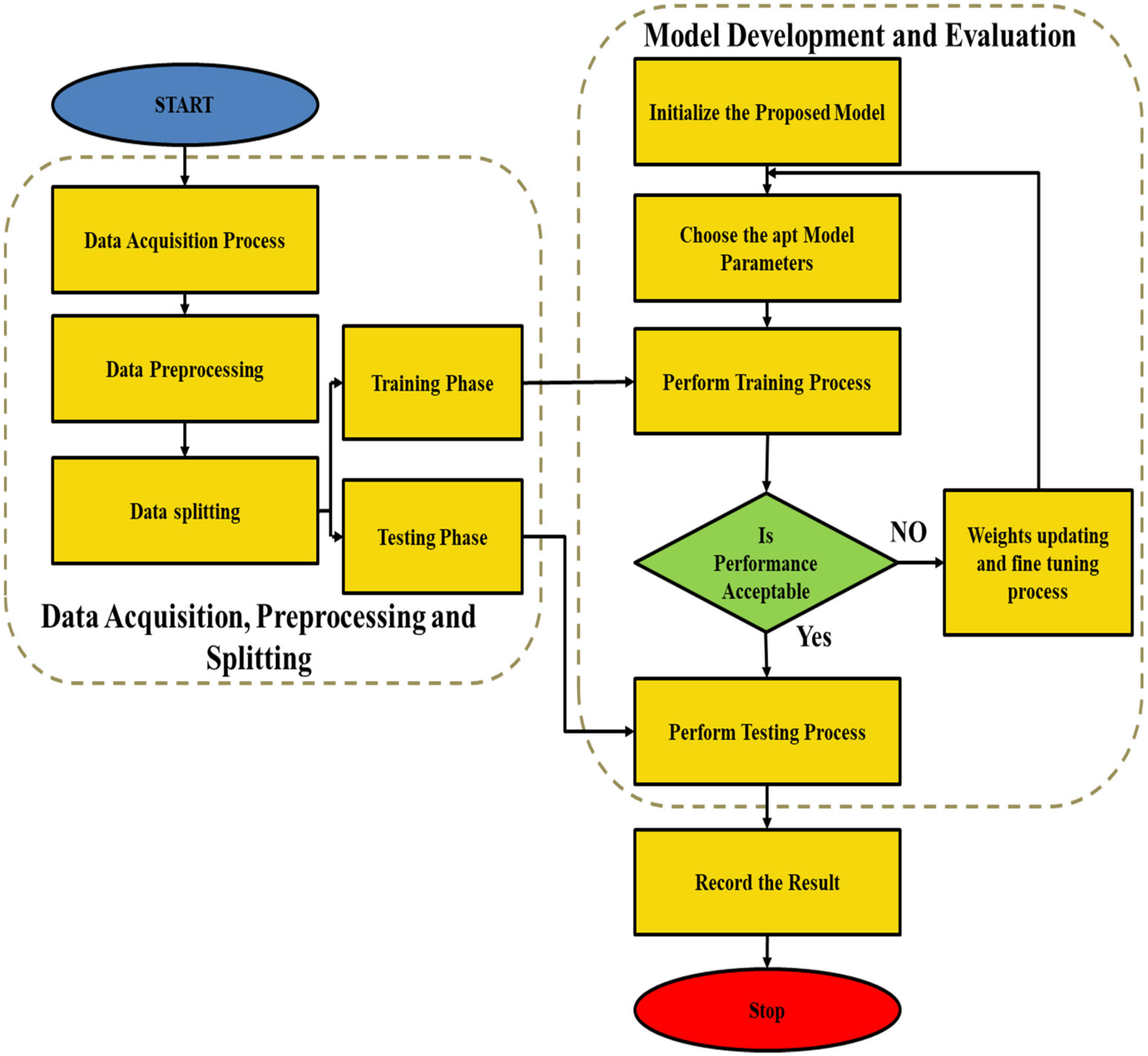
Electricity load forecast depends on various factors such as geographical location, atmospheric weather conditions, types of days and seasons, subsidies, and energy tariffs. Hence, it possesses irregularities and uncertainty; it creates demanding and challenging tasks for accurate electricity load forecasting. This paper endeavors an electricity load forecasting model using a multilayer perceptron neural network; the proposed model was experimentally conducted on the MATLAB platform. The proposed forecasting model was run on an Acer laptop with a Pentium (R) dual-core processor of 2.30 GHz, RAM: 2 GB. The presented forecasting model’s performance was validated using ERCOT data sets. ERCOT data sets and ENTSO-E data sets with different input parameters are collected and used as training and testing sets.
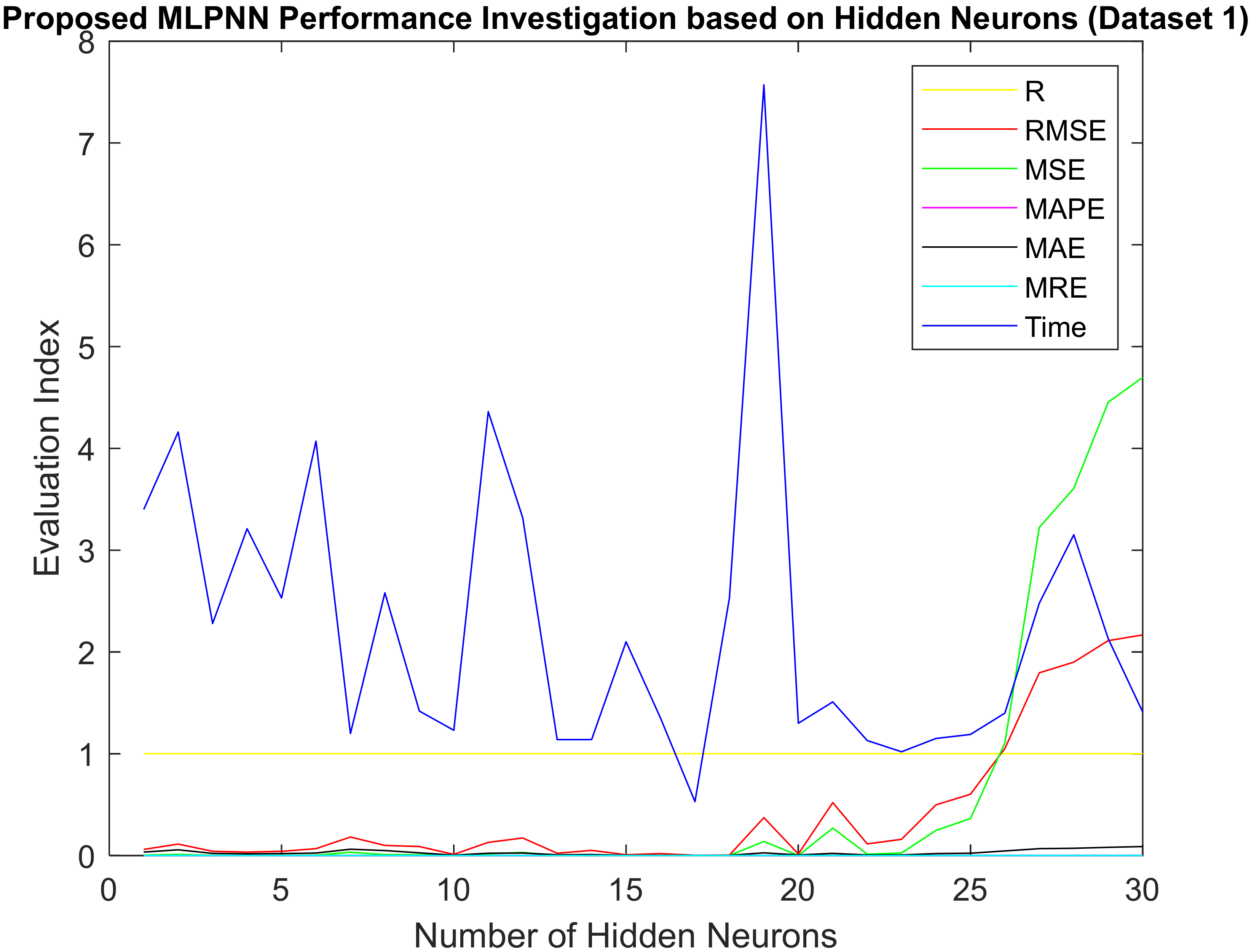
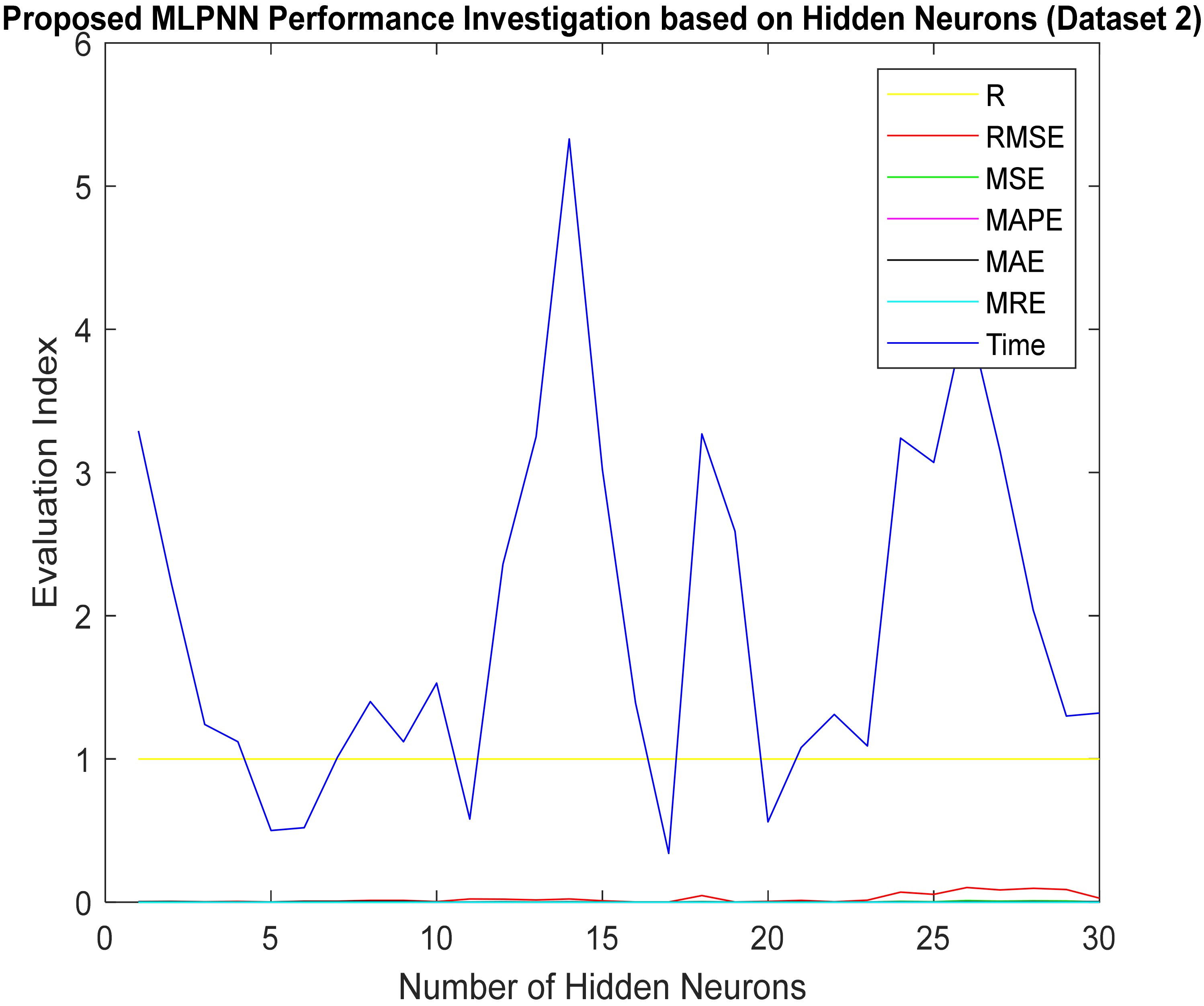
The hidden neurons possess a critical role in the artificial neural network’s stability and accuracy; improper selection of hidden neurons leads to poor performance, underfitting, and overfitting problems. Hence, this paper carried out a performance investigation concerning the various hidden neuron placements in the hidden layer of the proposed multilayer perceptron neural network to resolve the hidden neurons’ issues. The proposed model-based results regarding various hidden neurons concern the electricity load forecasting tabulated in Table 3 and Table 4.
The number of hidden neurons that influence the neural network is understood clearly from Table 3 and Table 4, Figure 4 and Figure 5, respectively, for Dataset 1 and Dataset 2, which shows that the hidden neurons are essential in neural network stability, and convergence.
From the careful investigation of Table 3 and Table 4, it is noted that the proposed model with 17 hidden neurons in the hidden layer achieves the minimal evaluation index as RMSE = 0.0034, MSE = 1.1506 × 10−05, MAPE = 2.3633 × 10−05, MAE = 0.0021, MRE = 2.3633 × 10−07 and R = 1, convergence time is 0.53 min for dataset 1, RMSE = 6.3358 × 10−04, MSE = 4.0142 × 10−07, MAPE = 7.5578 × 10−05, MAE = 4.5615 × 10−04, MRE = 7.5578 × 10−07 and R = 1, convergence time is 0.34 min for dataset 2. Hence, this hidden neuron (17) was selected as the optimal hidden neuron. Further investigation concerning different forecasting horizons was performed based on the optimal hidden neurons based on the implemented proposed model.
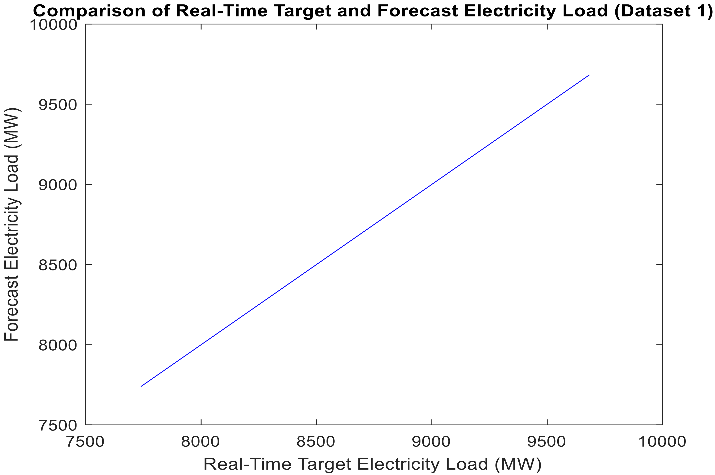
Table 5 and Figure 6 present the comparison of real-time and forecast electricity load (Dataset 1).
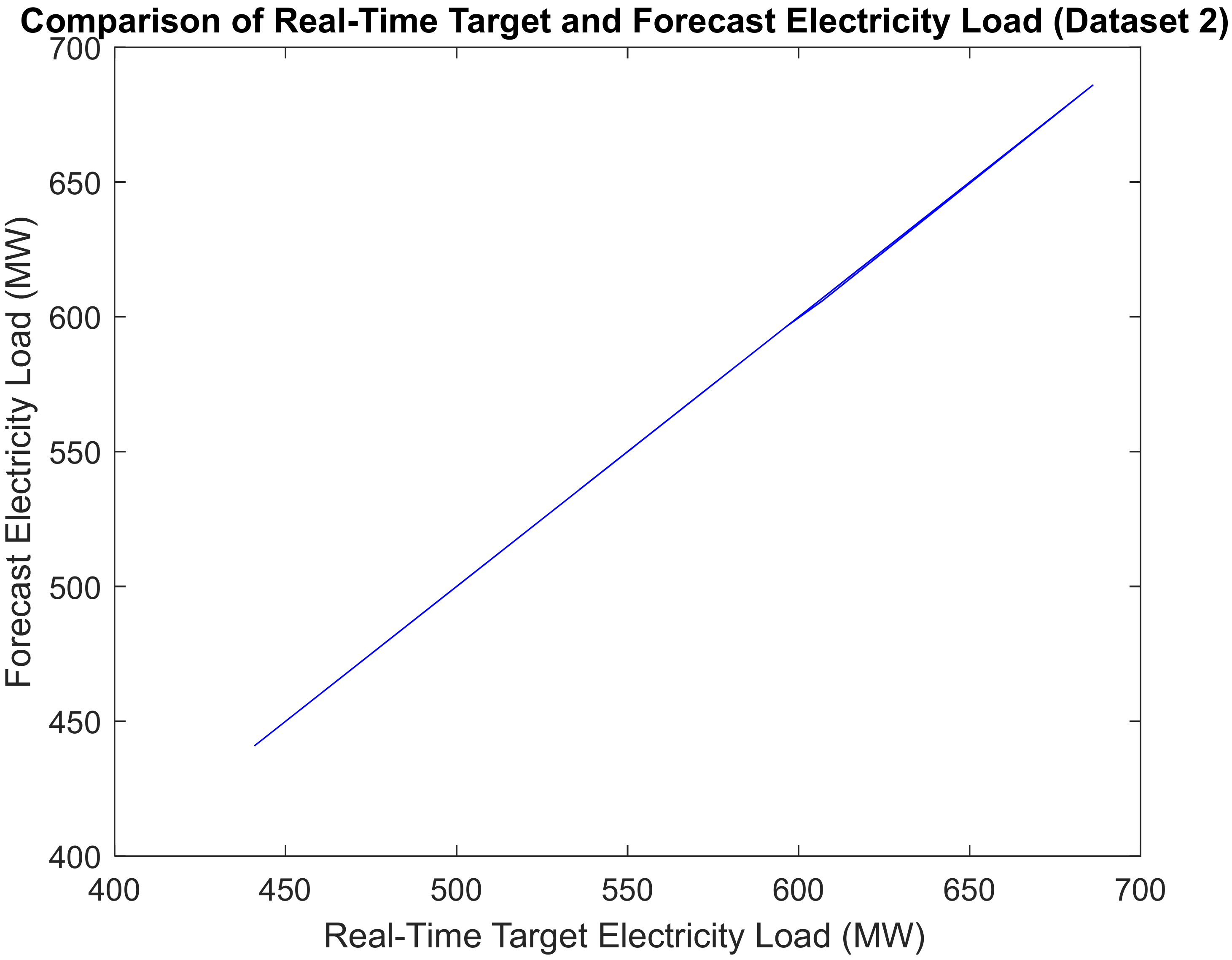
 Table 6 and Figure 7 depict the comparison of real-time and forecast electricity load (Dataset 2). As observed from the obtained simulation results shown in Table 5 and Table 6 and Figure 6 and Figure 7 is the proposed model to accurately match the forecast electricity load with the target real-time electricity load. It indicates the proposed model’s validity.
Decaying the power shortage issue and meeting the future electric energy requirement, different forecasting horizons based on electricity forecasting are obligatory. Our primary motive is to forecast the highly accurate load forecasting concern for various time horizons. The input electricity load depends on the time horizon forecast range. The output load is the ahead forecasting concern with different forecasting horizons compared with the real-time target load.
Long-term forecasting: The proposed long-term forecasting model can forecast the weekly/monthly/yearly ahead load forecast. Long-term load forecasting plays a significant role in power system planning, expansion, and operation management.
Medium-term load forecasting: The proposed medium-term load forecasting model forecasts 6 h to 24 h (1 day) ahead of the load forecast. Medium-term load forecasting is helpful for power system load scheduling, load balancing, reserve planning, and control.
Short-term load forecasting: The suggested short-term load forecasting model forecasts the load in 30 min to 6 h ahead of the load forecast. Short-term load forecasting is essential for unit commitment, economic dispatch, and the electricity market.
Very short-term load forecasting: The presented very short-term load forecasting covers a period of 1 min to 30 min ahead of the load forecast. Very short-term load forecasting is helpful for the deregulated power industry and energy prizing.
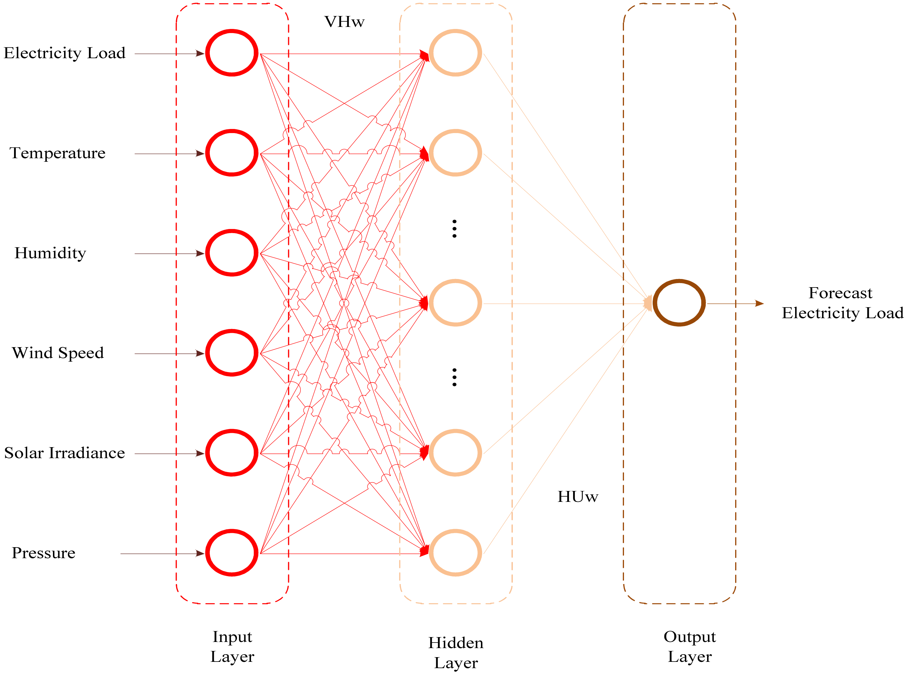
In this paper, the authors propose a different forecasting horizons model mentioned above, range or period ahead load forecasting, which overcomes the issues related to energy and load management and aids power system engineers. Although the authors already specified the proposed model inputs in Table 1 and Table 2 and 
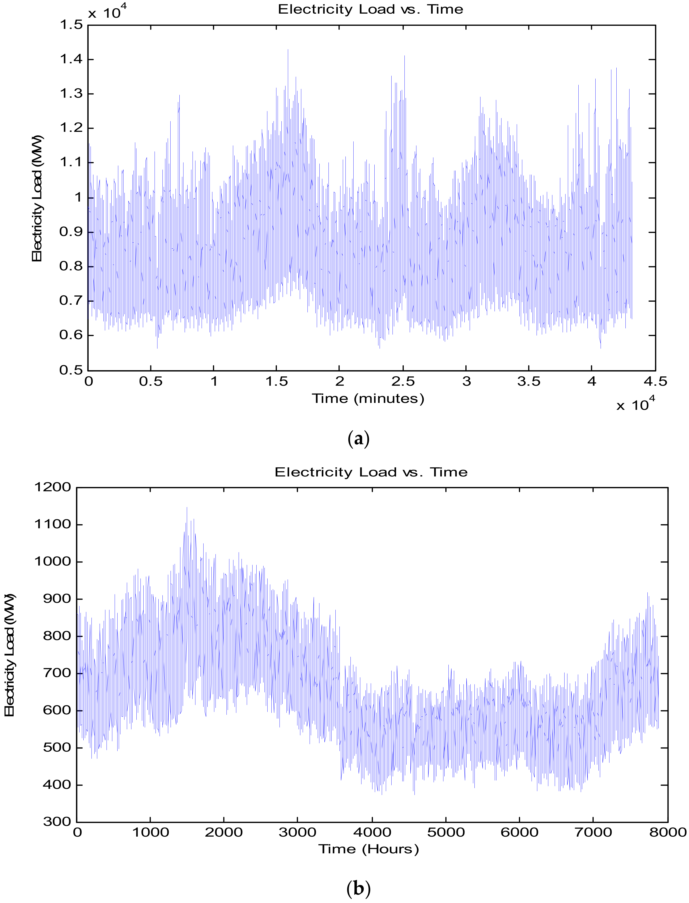
Figure 1 to make it clearly understood it was mentioned again as the proposed load forecasting model built based on six inputs, namely, electricity load (MW), temperature (°C), humidity (%), wind speed (m/s), solar irradiance (W/m), and pressure (bar). For Dataset 1 comprises 5.256 × 10⁶ data points of each taken input variable, and Dataset 2 shall comprise 7.884 × 10⁴ data points of each taken input variable. Depending on the time horizon, as mentioned above, the input time span varies.
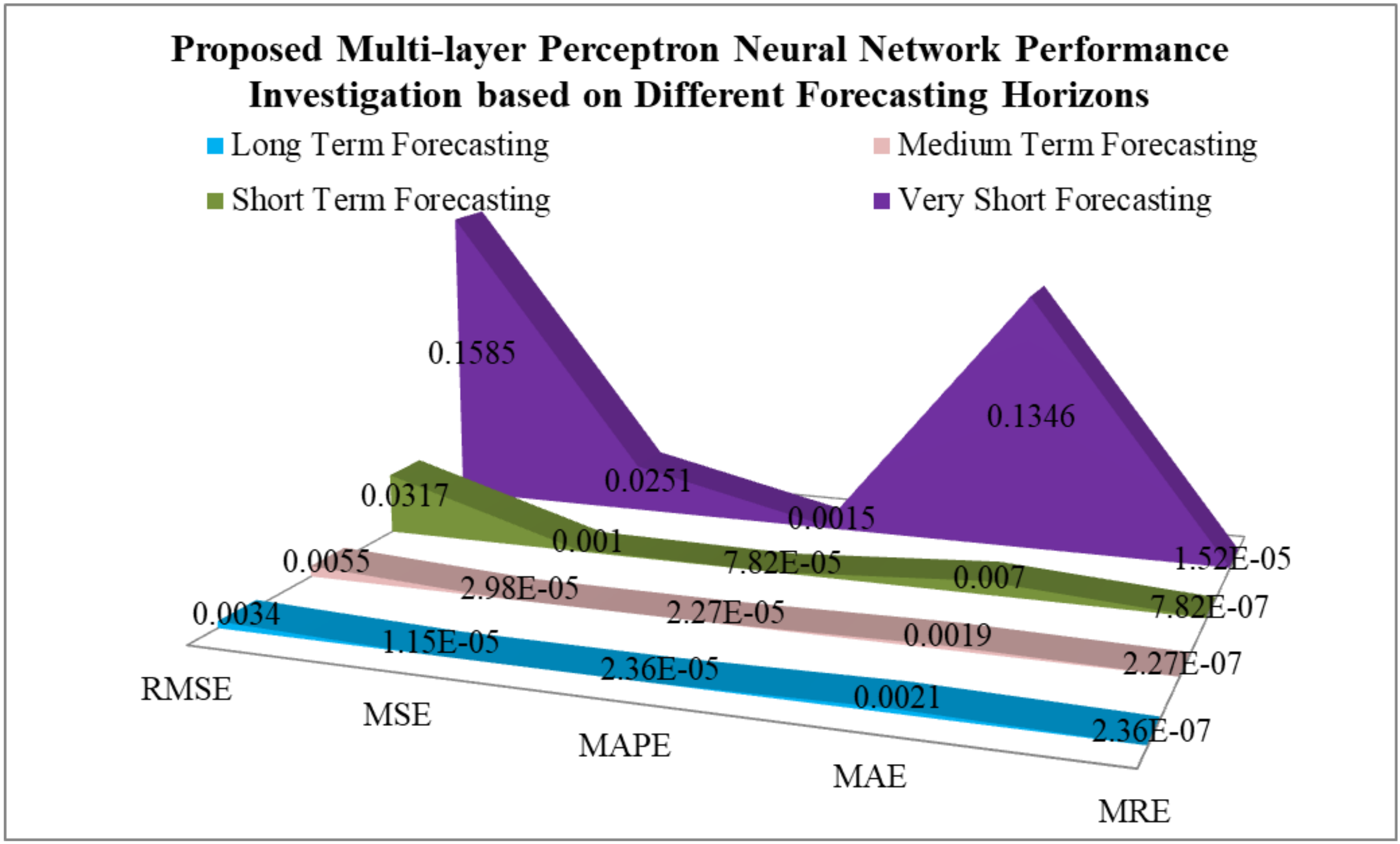
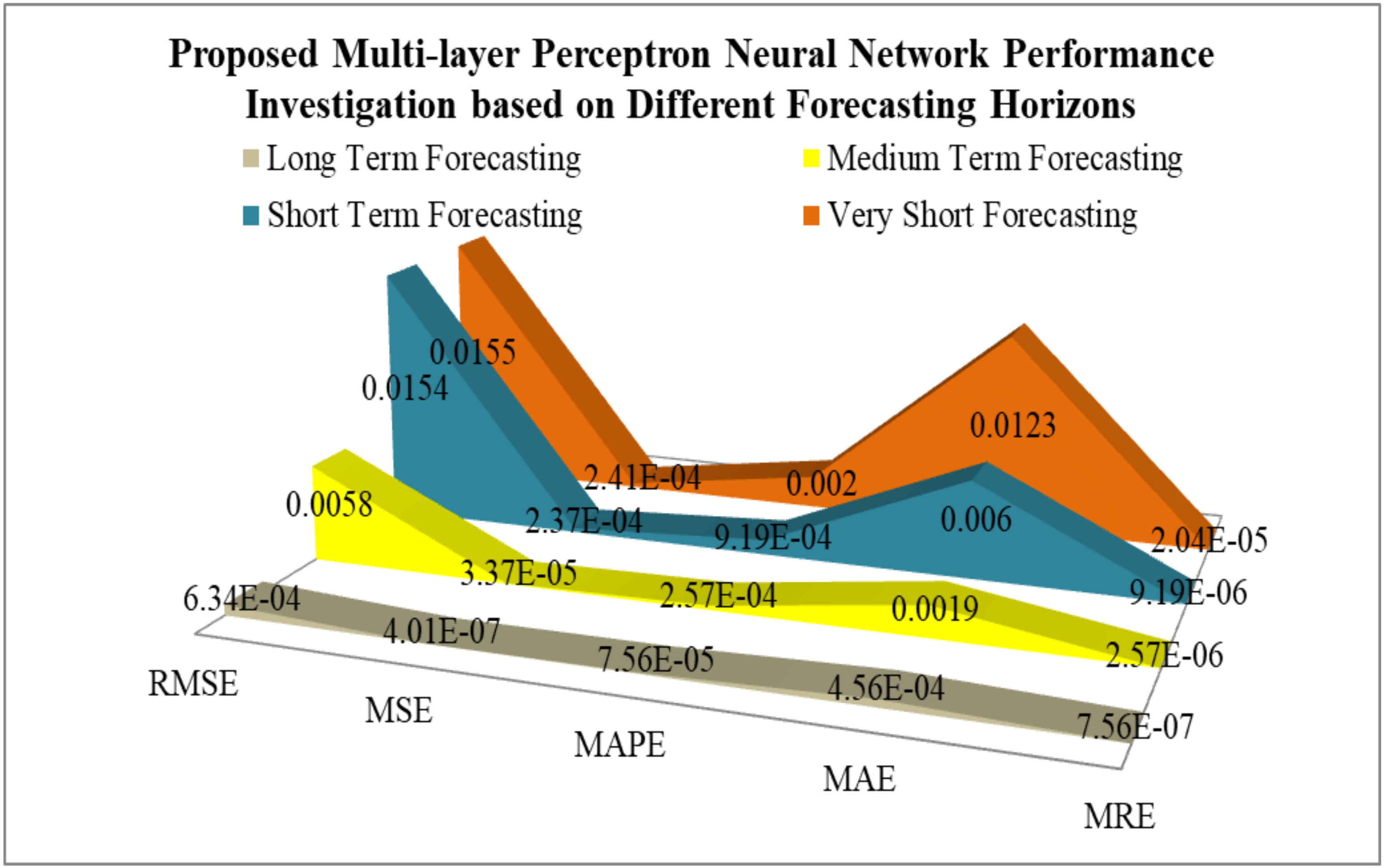
The horizon of long-term load forecasting is years ahead, the horizon of medium-term load forecasting is 24 h ahead, the horizon of short-term load forecasting is 6 h ahead, and the horizon of very short-term load forecasting is 30 min ahead. Therefore, the proposed multilayer perceptron neural network-based forecasting model performance was investigated with concern to the different forecasting horizons, namely long-term, medium-term, short-term, and very short-term electricity load forecasting. The obtained results based on the proposed model concern to different forecasting horizons presented in Table 7 and Table 8 show that the proposed model can forecast the electricity load in all time horizons, namely, long-term, medium-term, short-term, and very short-term, with minimum evaluation index (RMSE, MSE, MAPE, MAE, MRE) and converge faster for both datasets.
Figure 8, Figure 9 and 
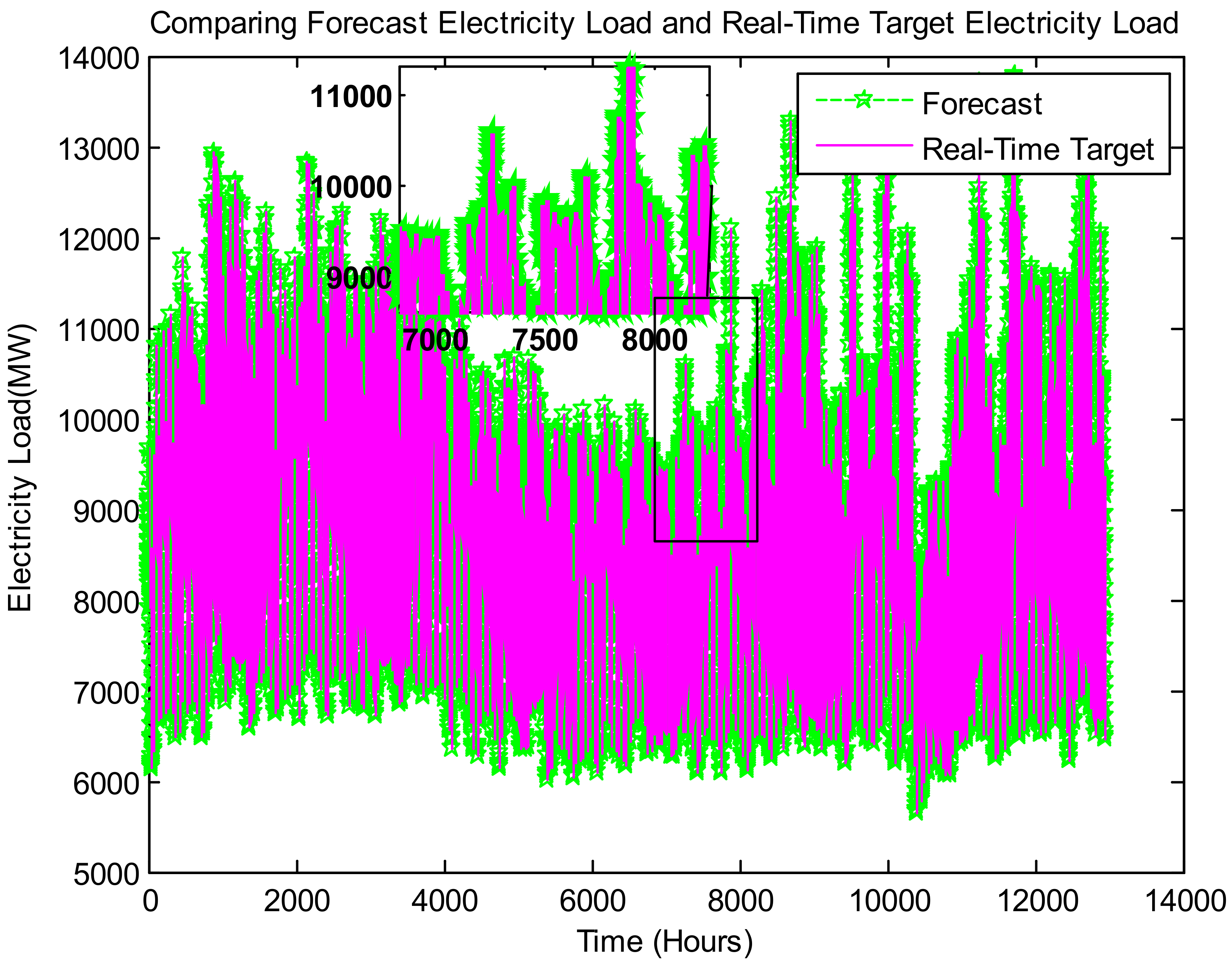
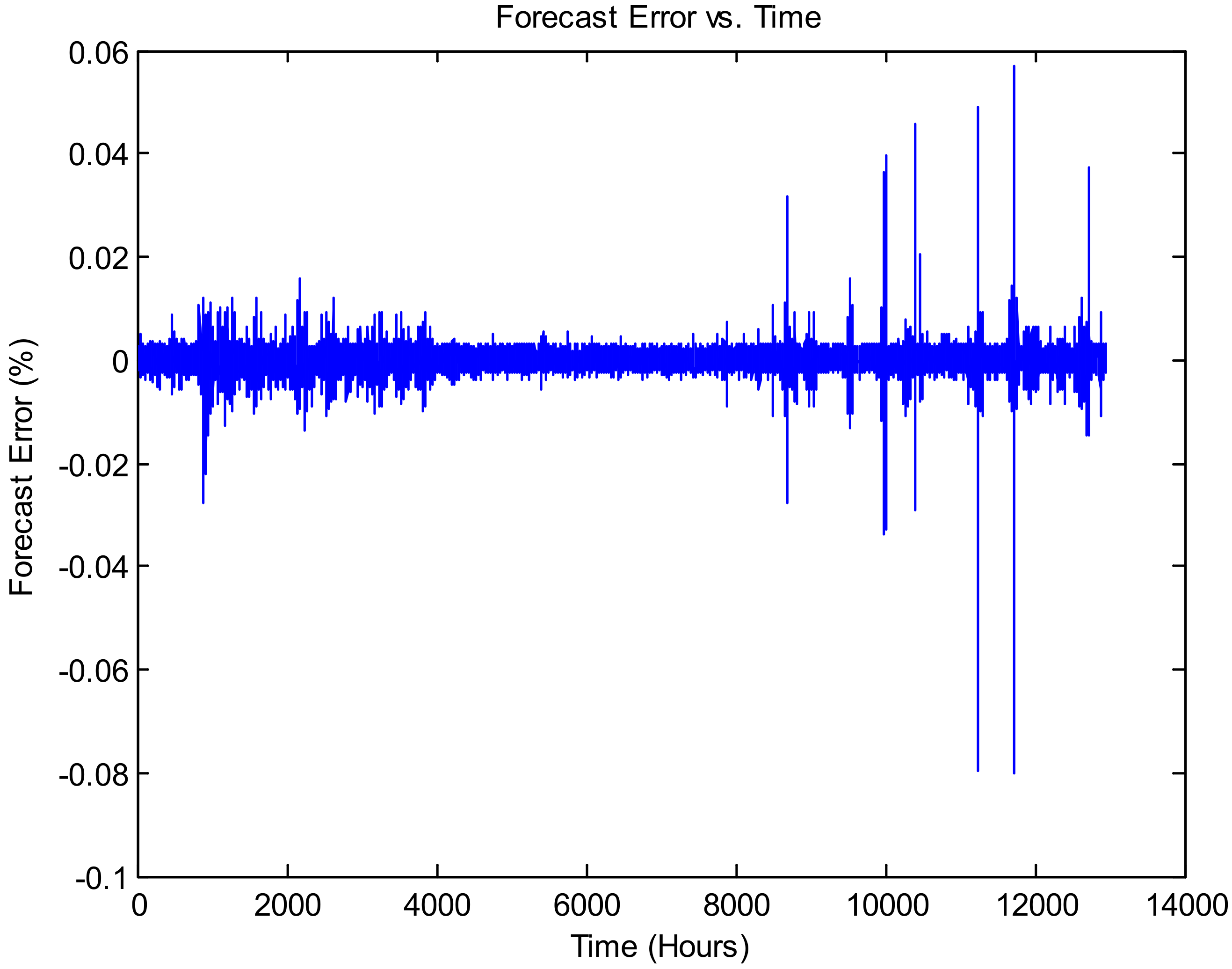
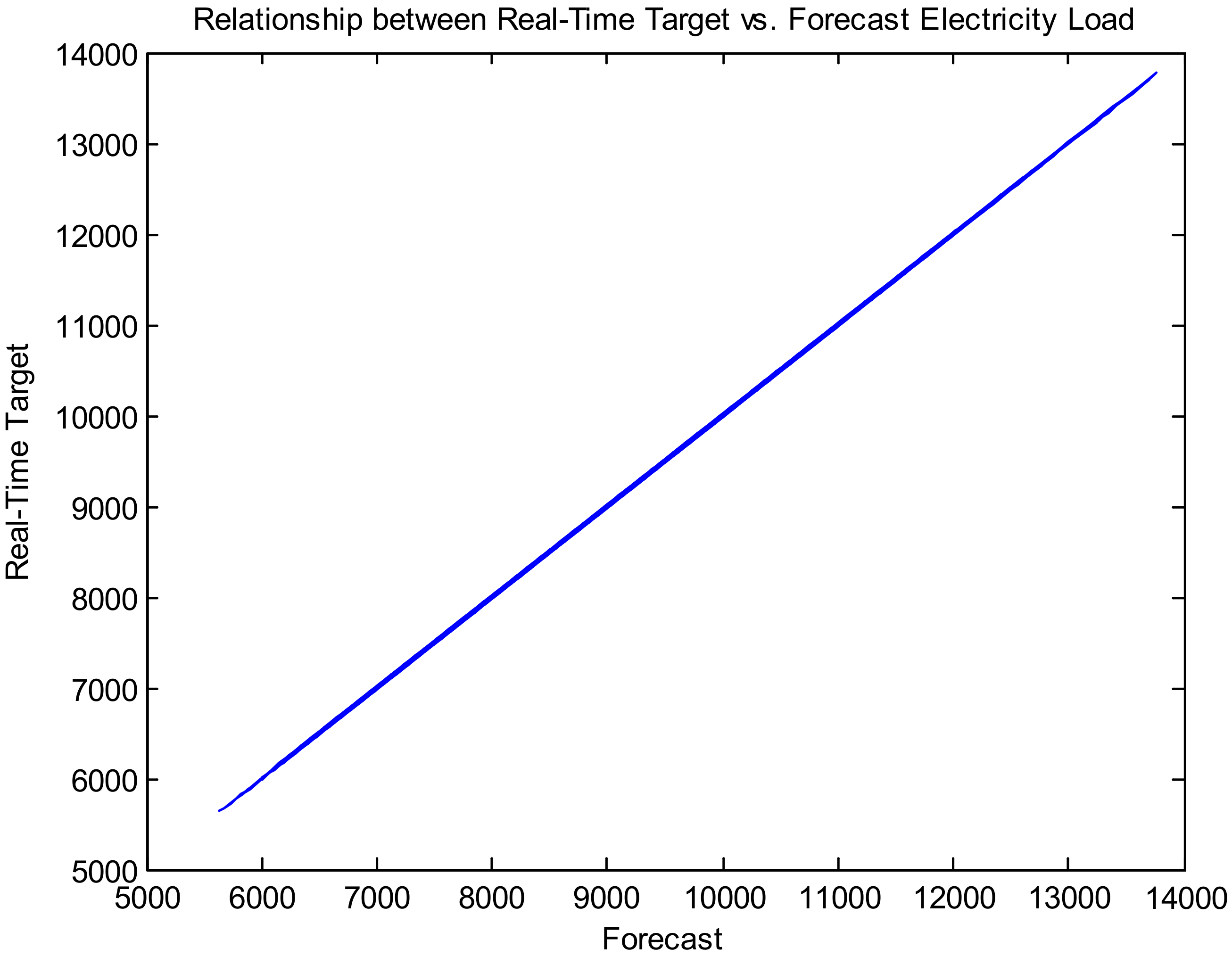
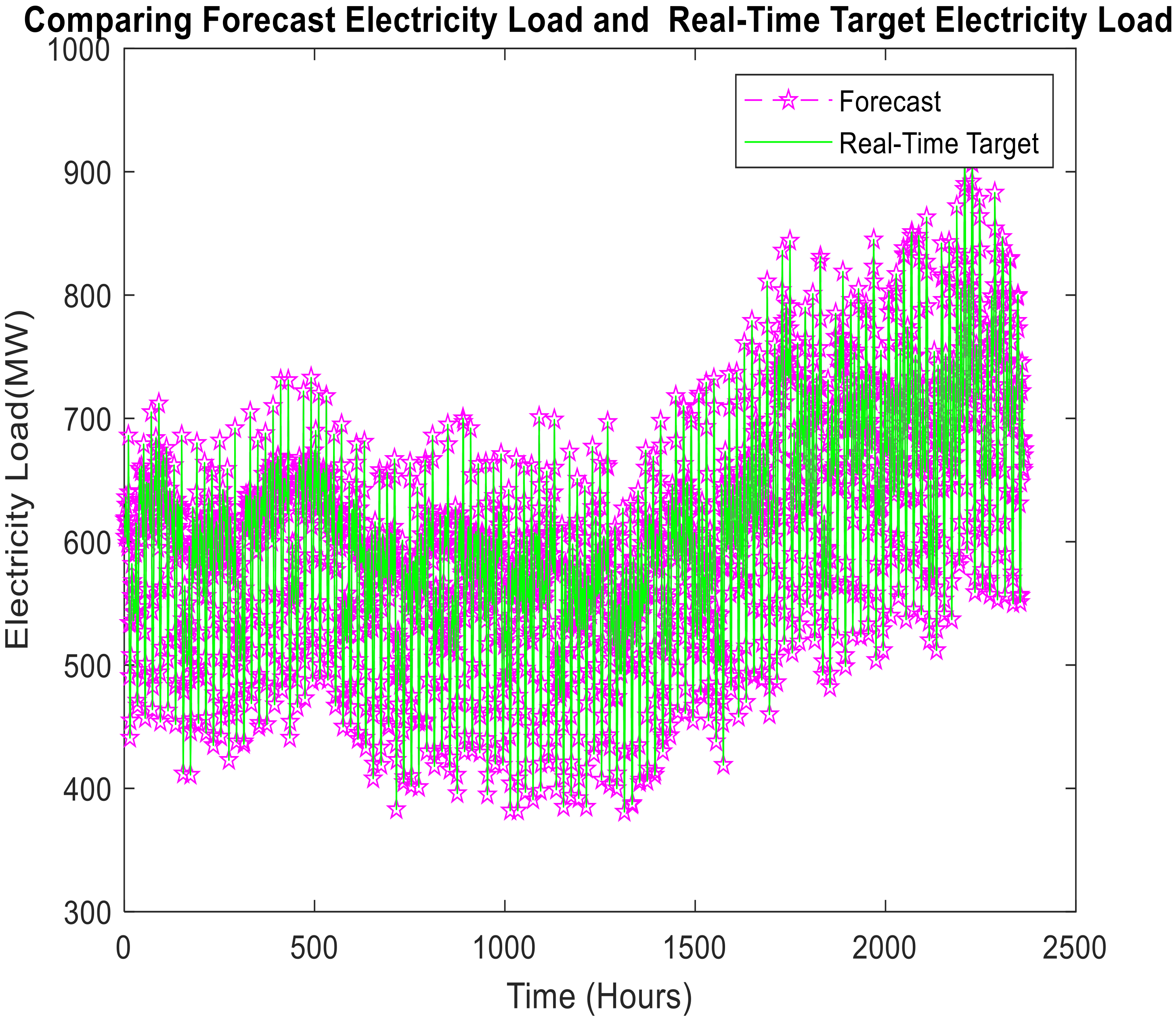
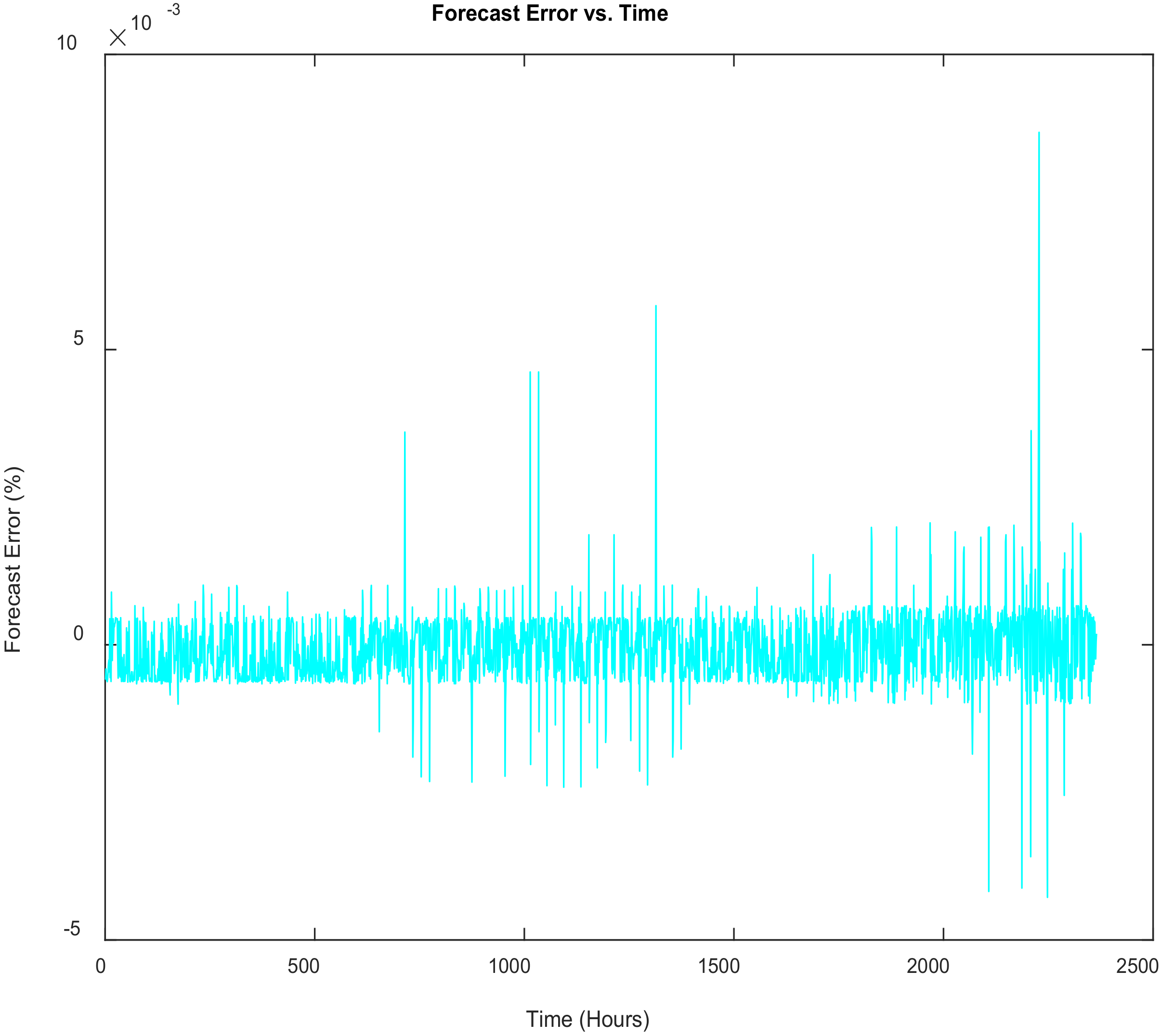
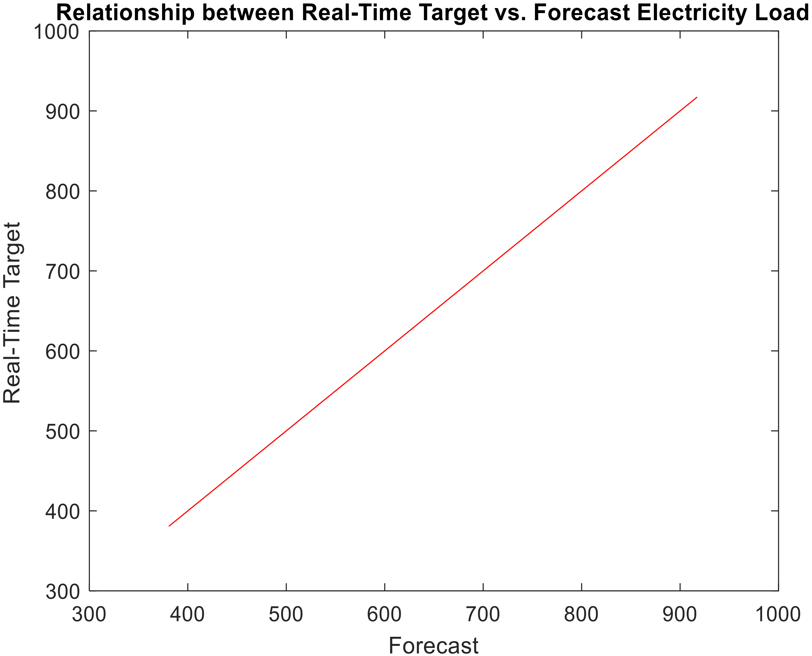
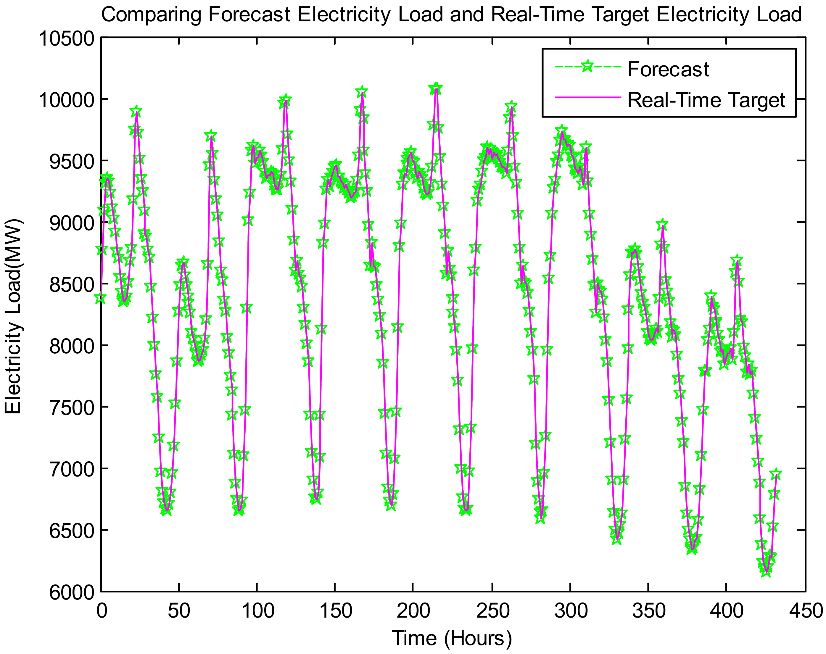
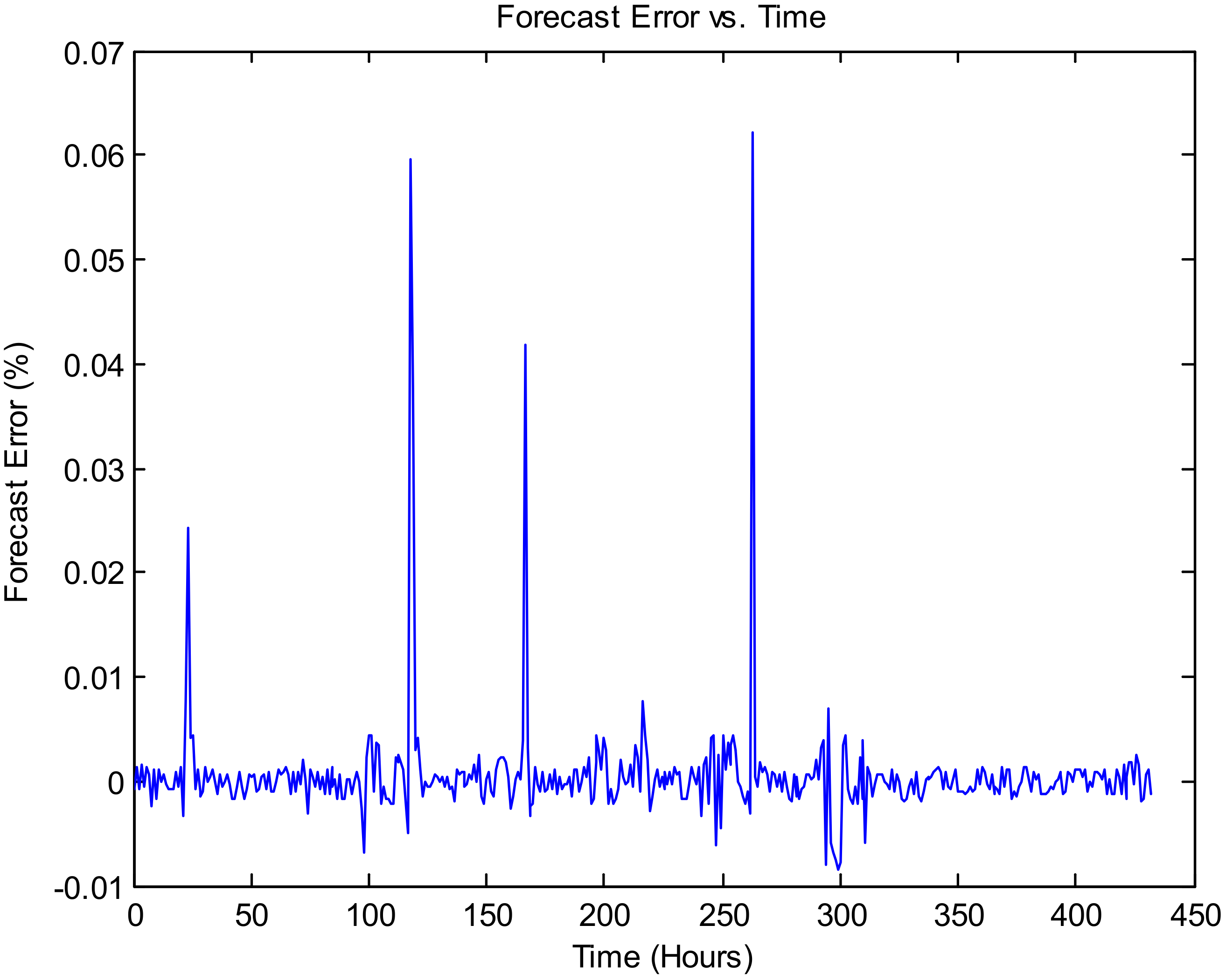
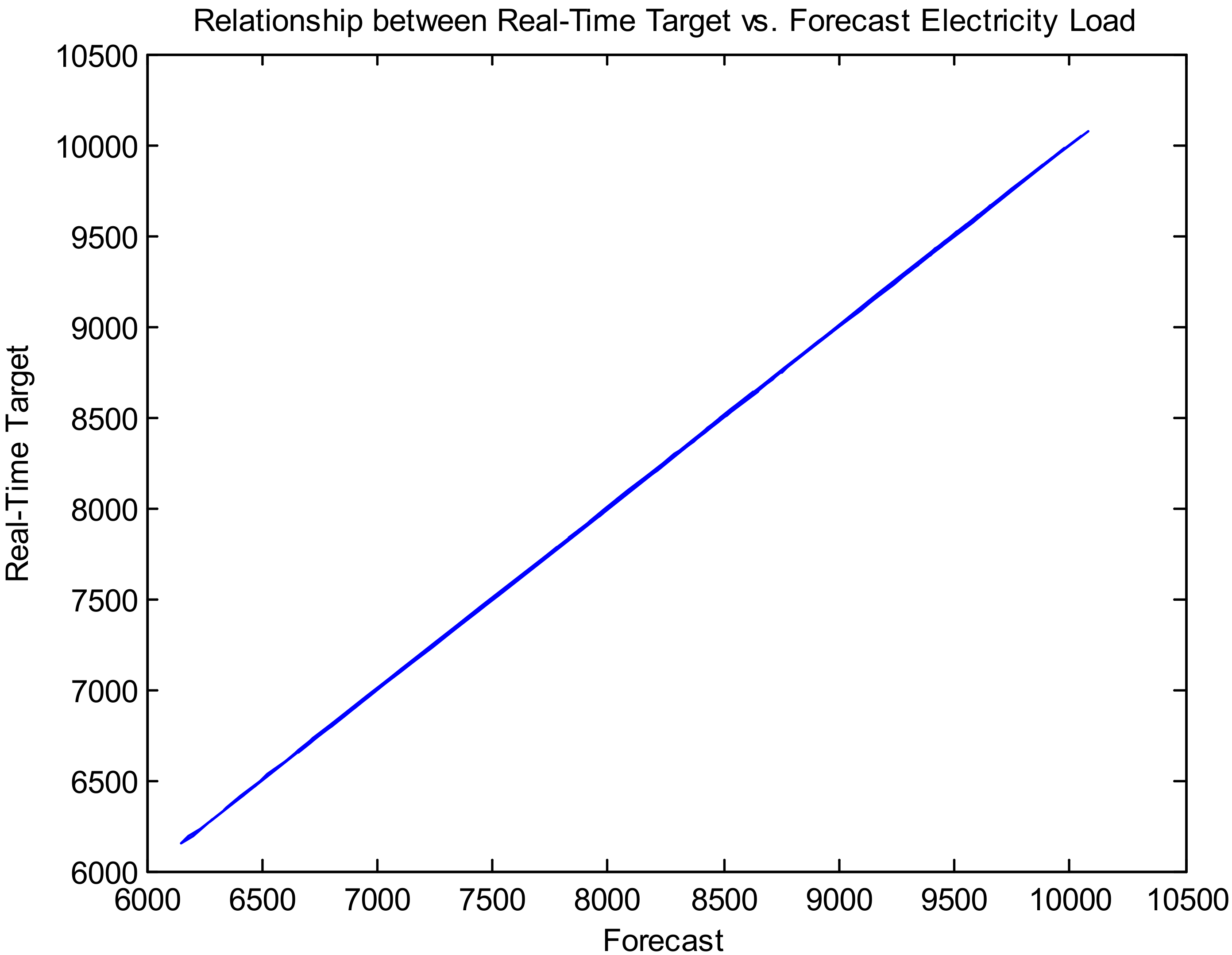
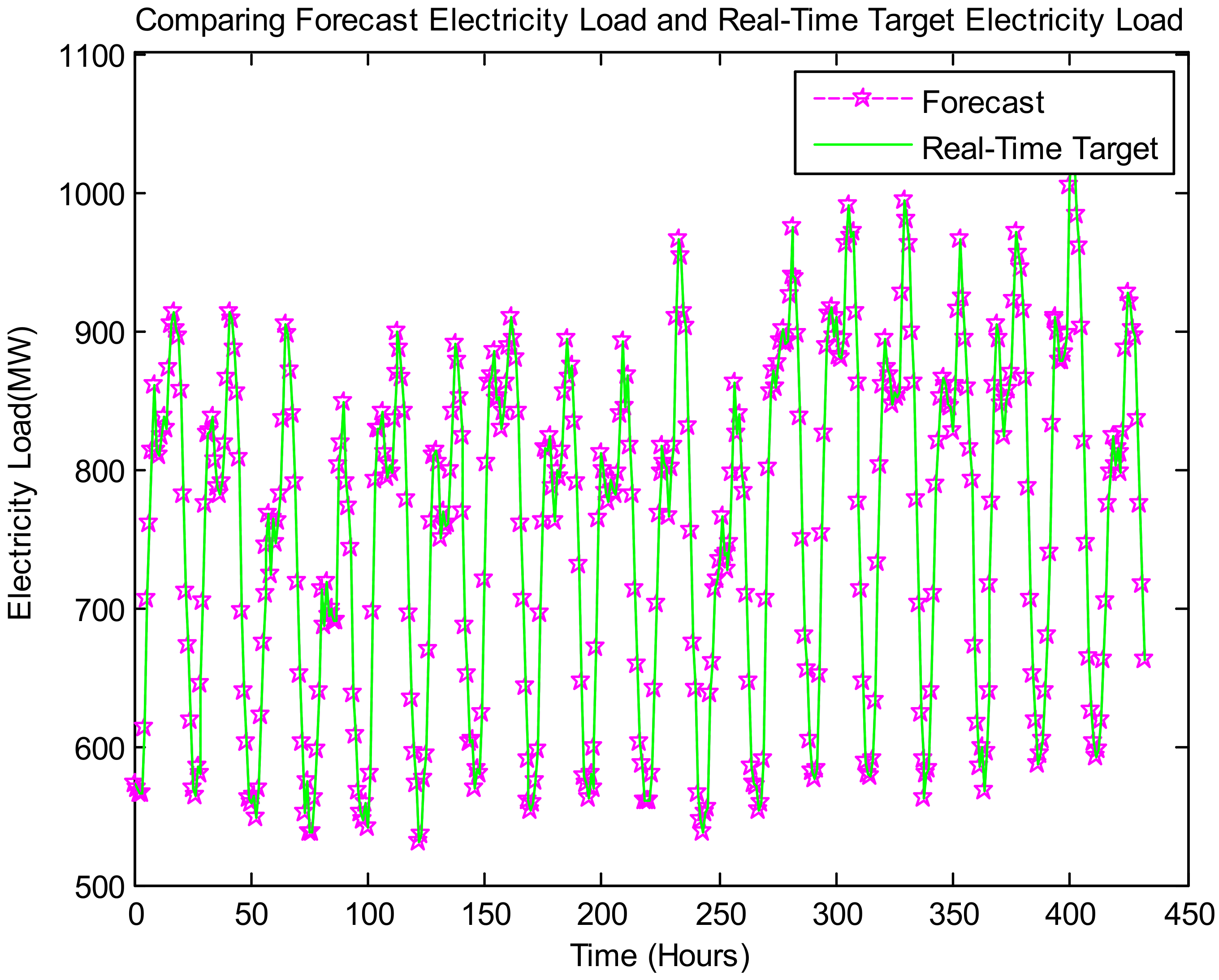
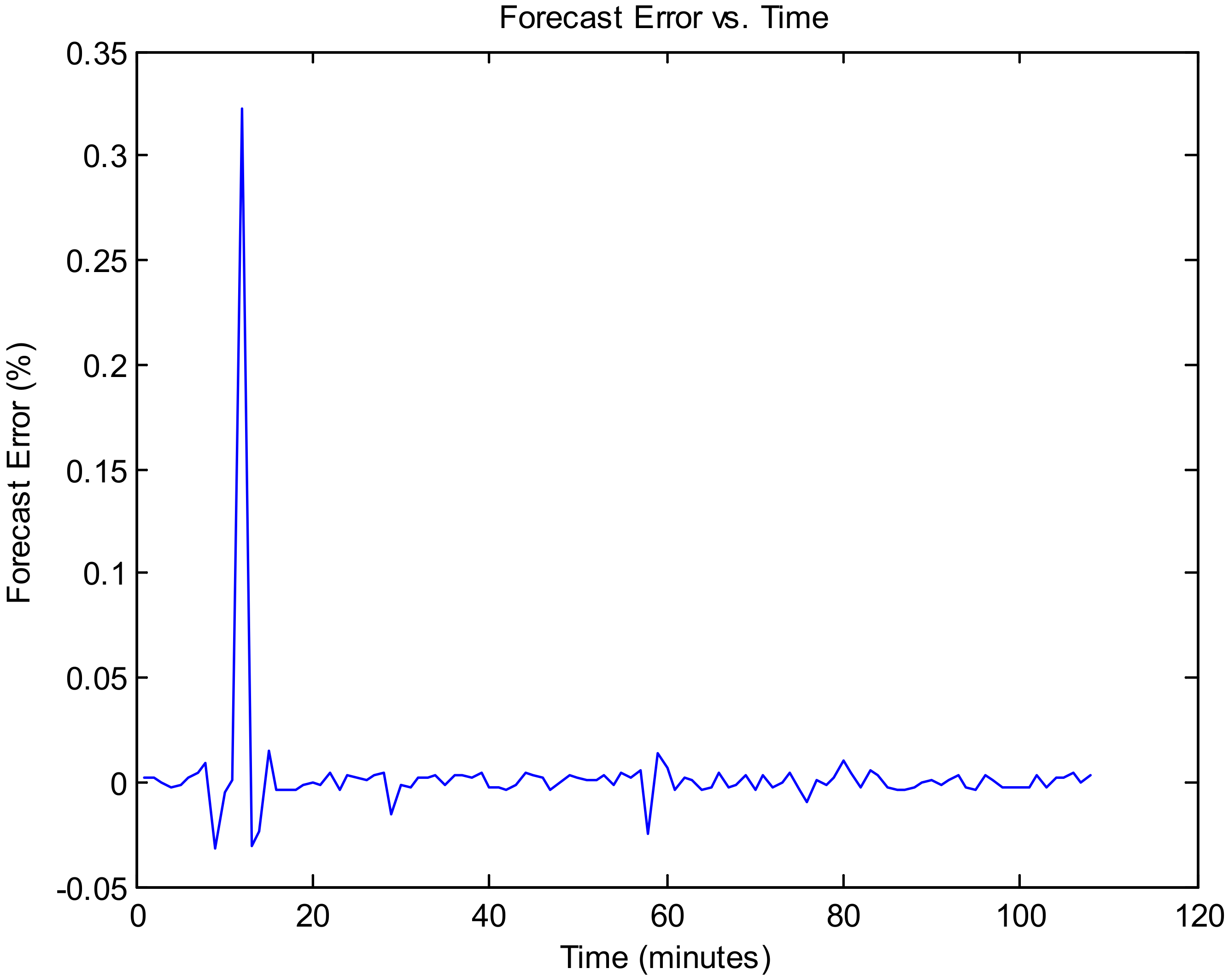
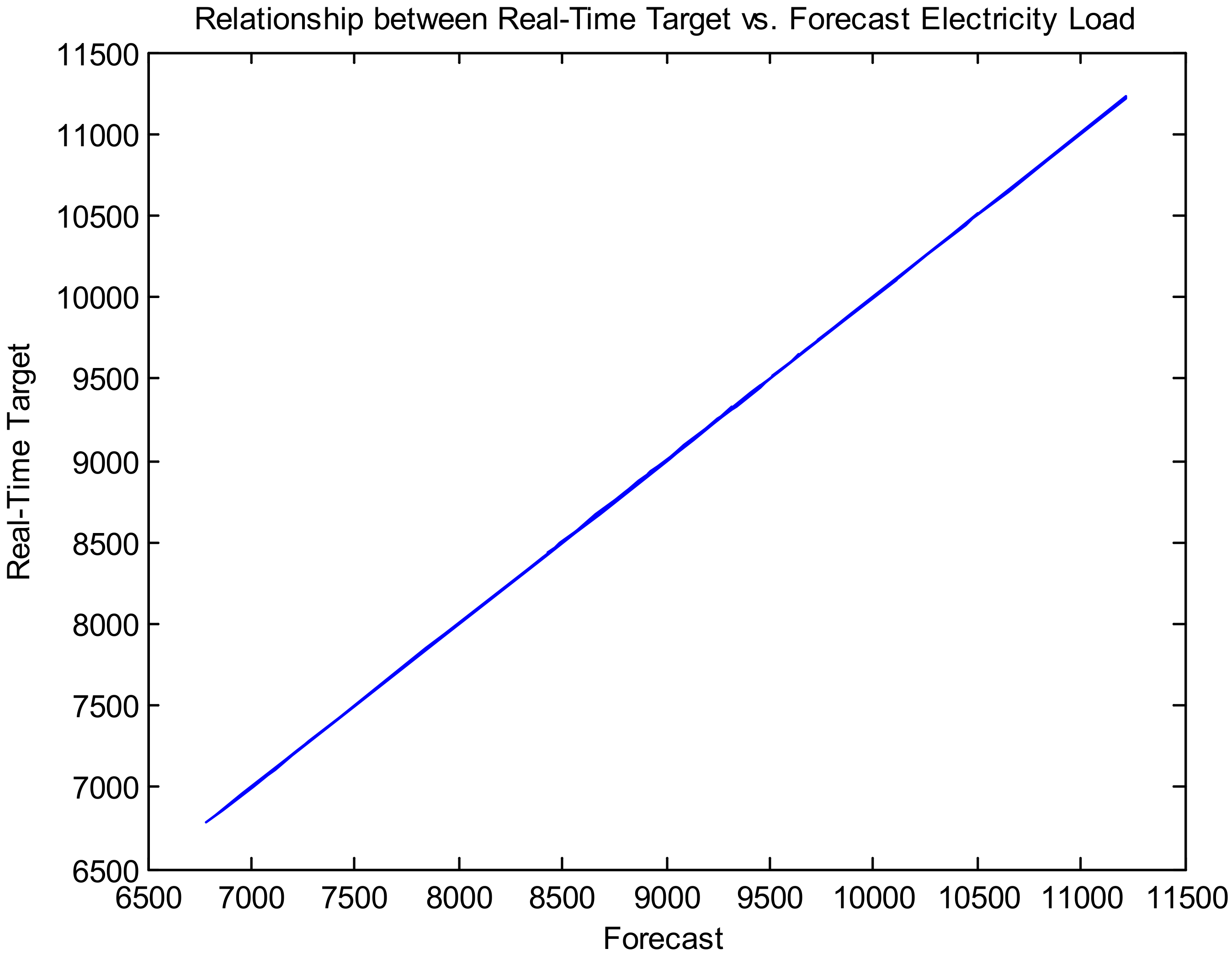
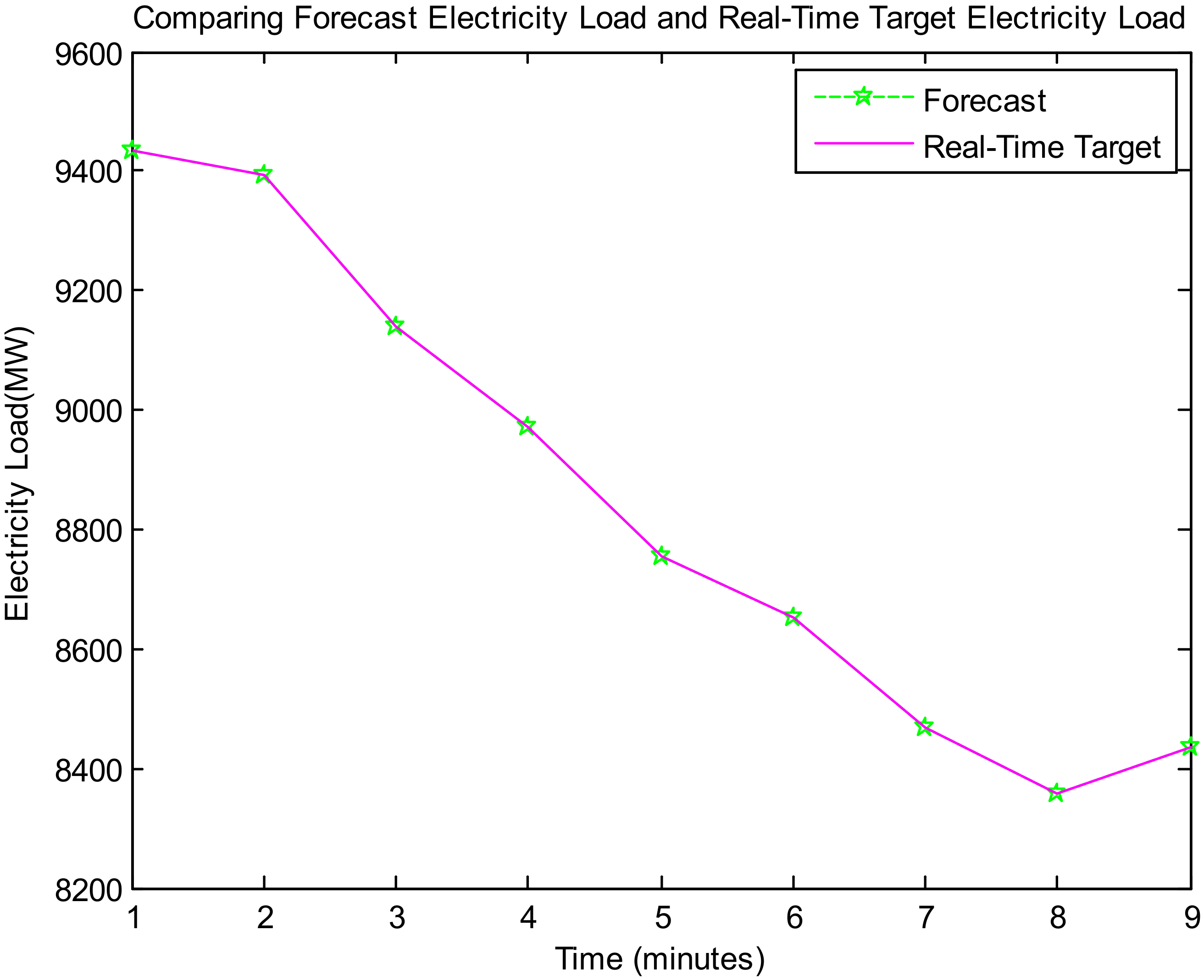
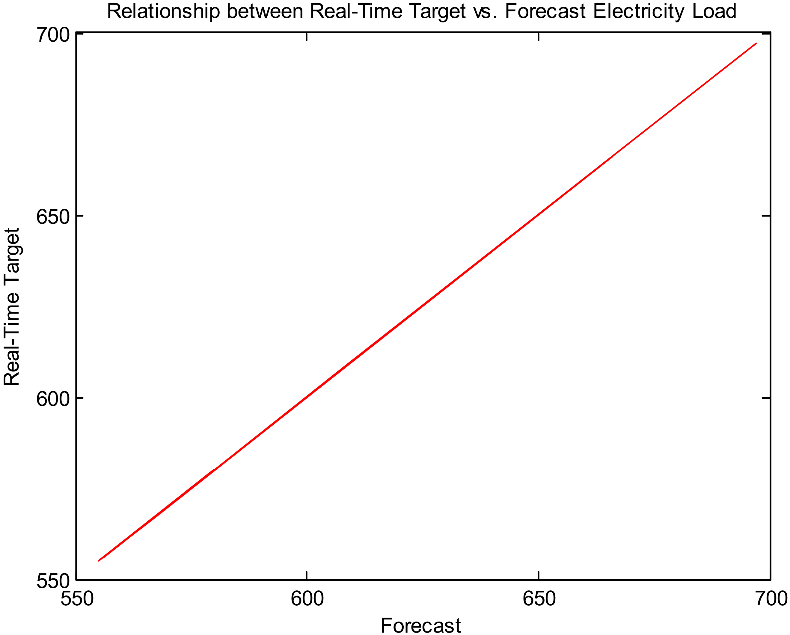
Figure 10 show the results of long-term load forecasting concern on dataset 1. Figure 8 represents the proposed model-based output, namely, comparing the forecast electricity load with real-time target electricity load in the horizon of years ahead. 
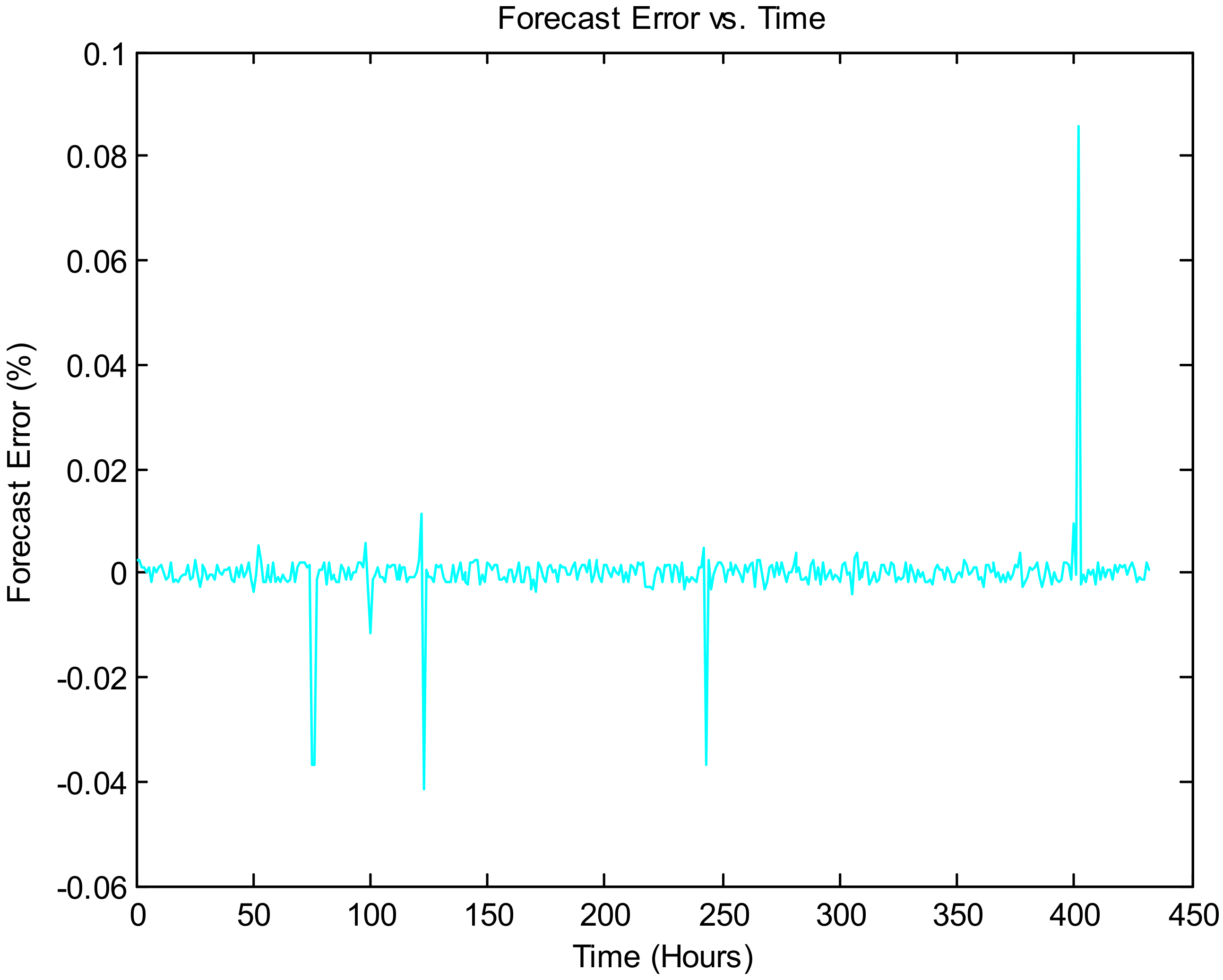
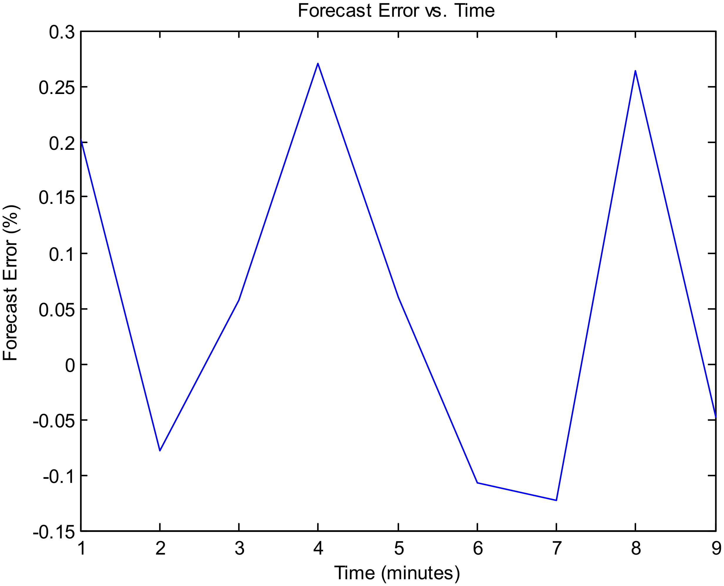
Figure 9 illustrates the forecasting error vs. time, and 
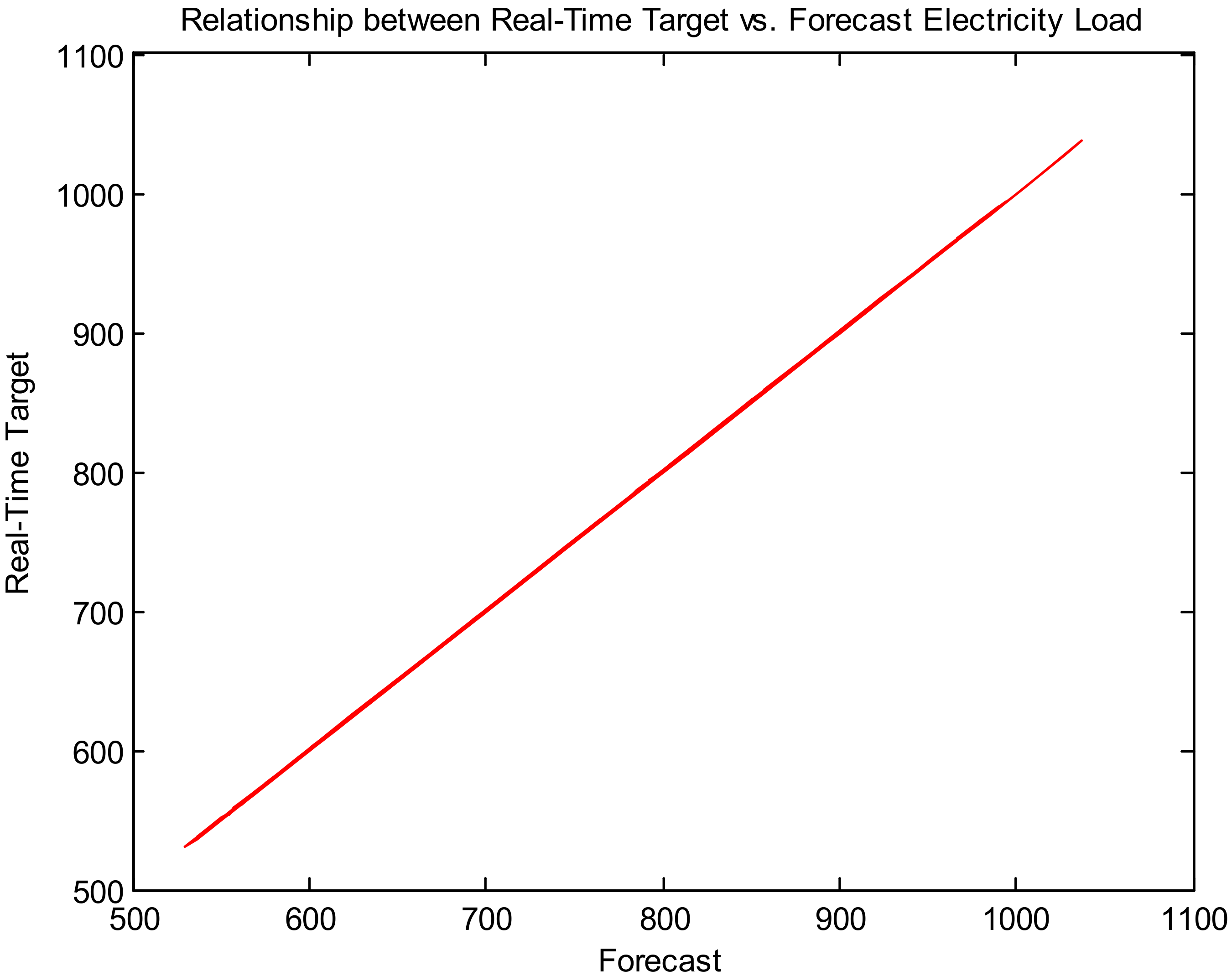
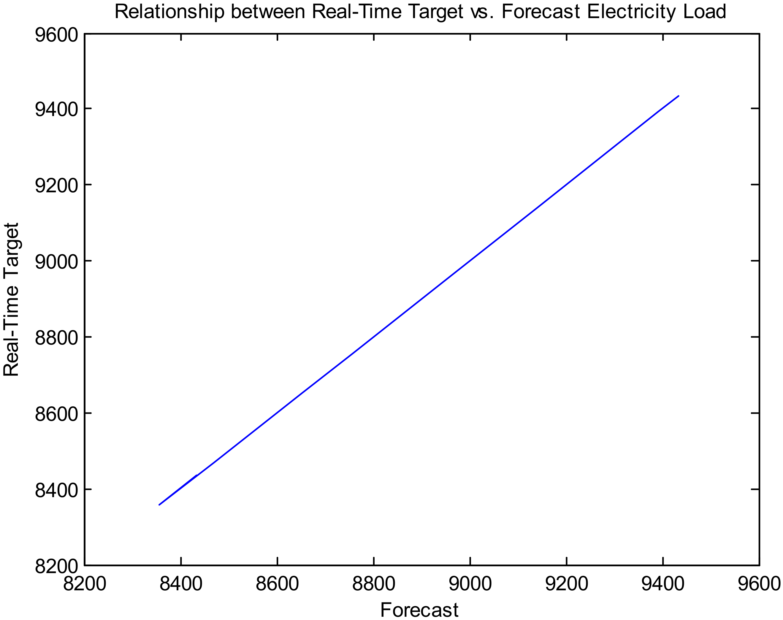
Figure 10 presents the relationship between real-time target and forecast electricity load for a long-term time horizon (dataset 1). Figure 11, Figure 12 and 
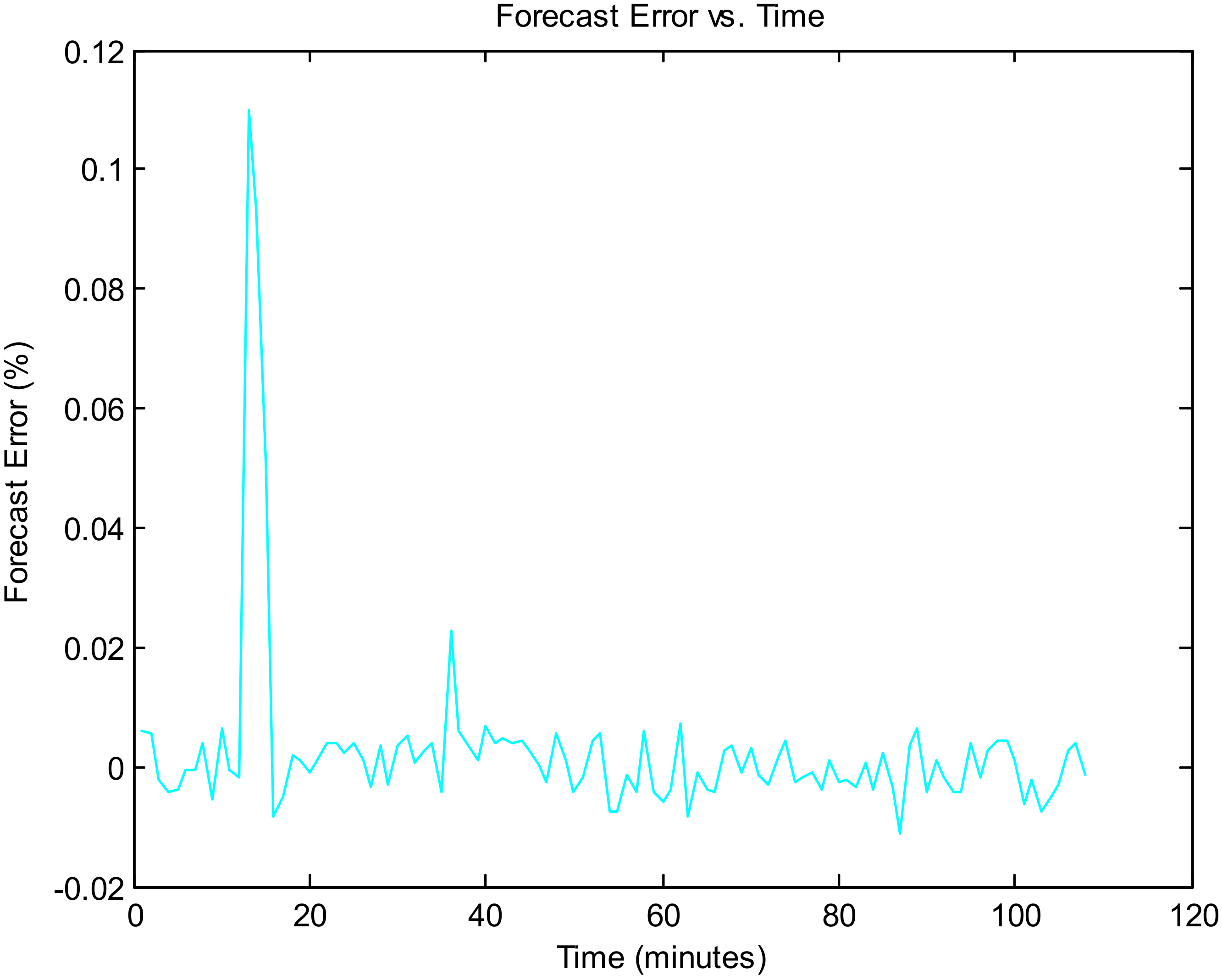
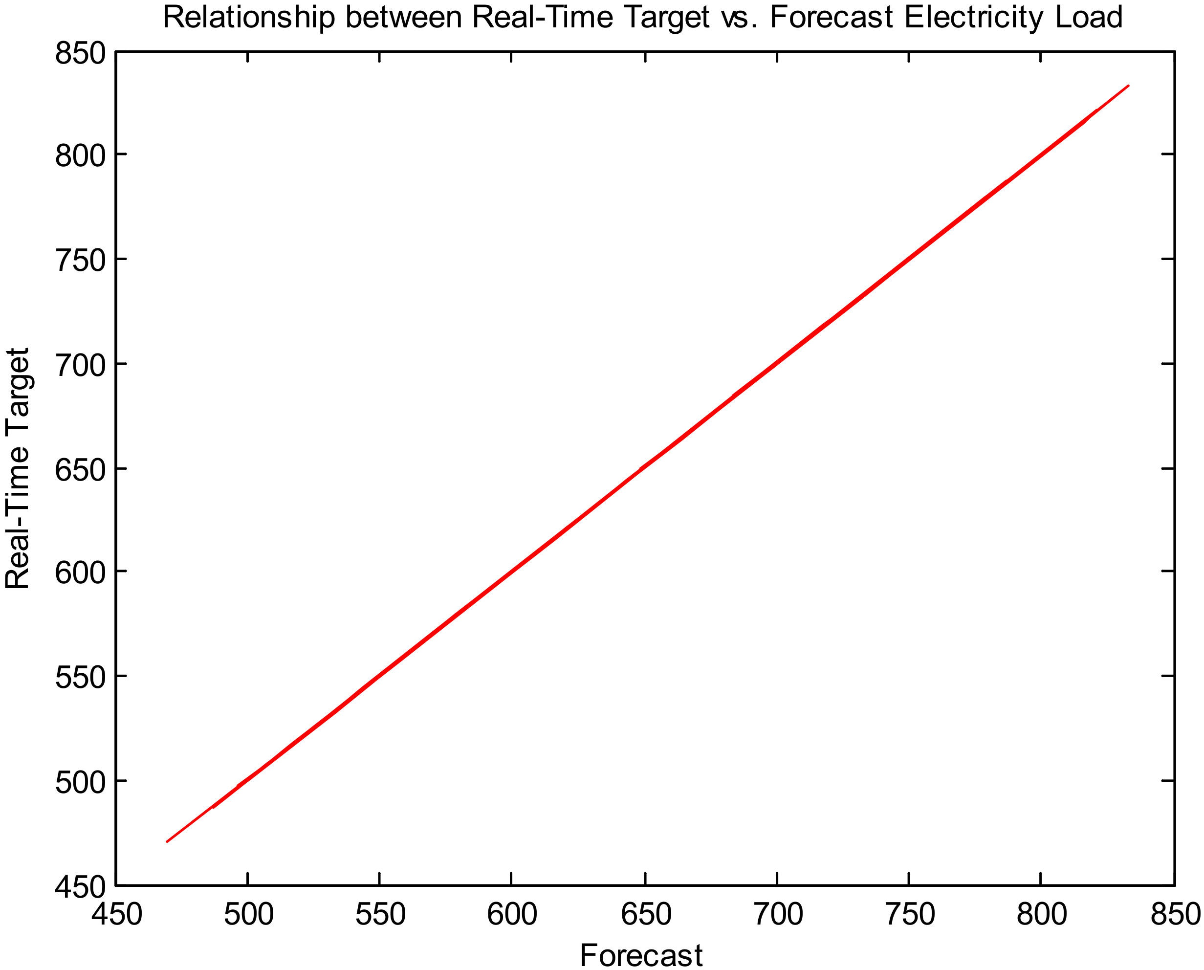
Figure 13 show the results of long-term load forecasting concern on Dataset 2. Figure 11 represents the proposed model-based output, namely, comparing the forecast electricity load with real-time target electricity load in the horizon of years ahead. 
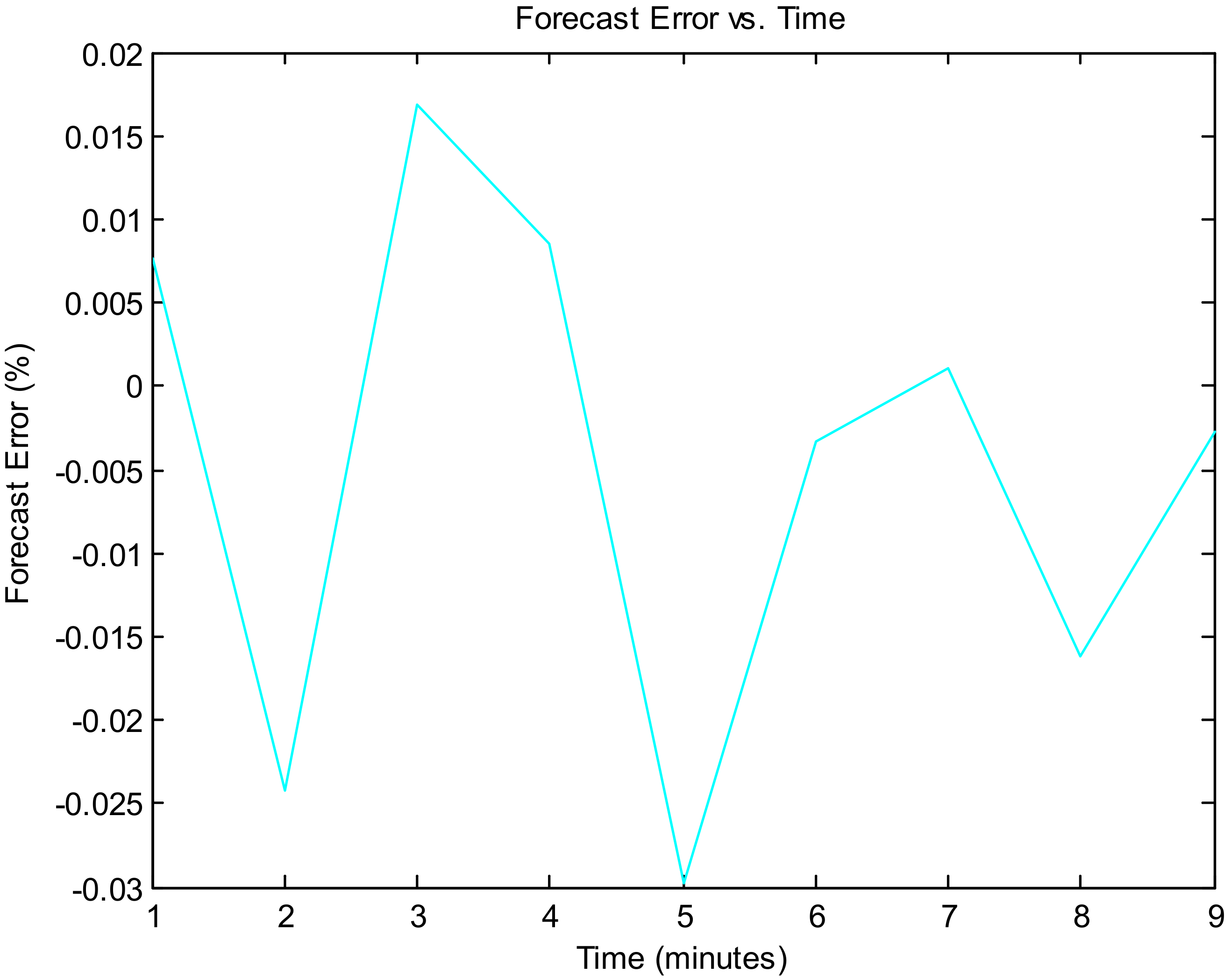
Figure 12 shows the forecasting error vs. time, and Figure 13 depicts the relationship between the real-time target and the forecast electricity load for a long-term time horizon (Dataset 2).
Similarly, Figure 14, Figure 15 and Figure 16 show the results of medium-term load forecasting concern on Dataset 1. Figure 14, Figure 15 and Figure 16 represent the proposed model-based output on Dataset 1, namely, comparing the forecast electricity load with real-time target electricity load in the horizon of 24 h ahead, forecasting error vs. time, and the relationship between real-time target and forecast electricity load for a medium-term time horizon, respectively (Dataset 1). Figure 17, Figure 18 and Figure 19 show the results of medium-term load forecasting concern on Dataset 2. Figure 17, Figure 18 and Figure 19 represent the proposed model-based output on Dataset 2, namely, comparing the forecast electricity load with real-time target electricity load in the horizon of 24 h ahead, forecasting error vs. time, and the relationship between real-time target and forecast electricity load for a medium-term time horizon, respectively (Dataset 2).
Figure 20, Figure 21 and Figure 22 show the results of short-term load forecasting concern on Dataset 1. Figure 20, Figure 21 and Figure 22 represents the proposed model-based output on Dataset 1, namely, comparing the forecast electricity load with real-time target electricity load in the horizon of 6 h ahead, forecasting error vs. time, and the relationship between real-time target and forecast electricity load for a short-term time horizon (Dataset 1). Figure 23, Figure 24 and Figure 25 show the results of short-term load forecasting concern on Dataset 2. Figure 23, Figure 24 and Figure 25 represents the proposed model-based output on Dataset 2, namely, comparing the forecast electricity load with real-time target electricity load in the horizon of 6 h ahead, forecasting error vs. time, and the relationship between real-time target and forecast electricity load for a short-term time horizon (Dataset 2).
Figure 26, Figure 27 and Figure 28 show the results of very short-term load forecasting concern on dataset 1.
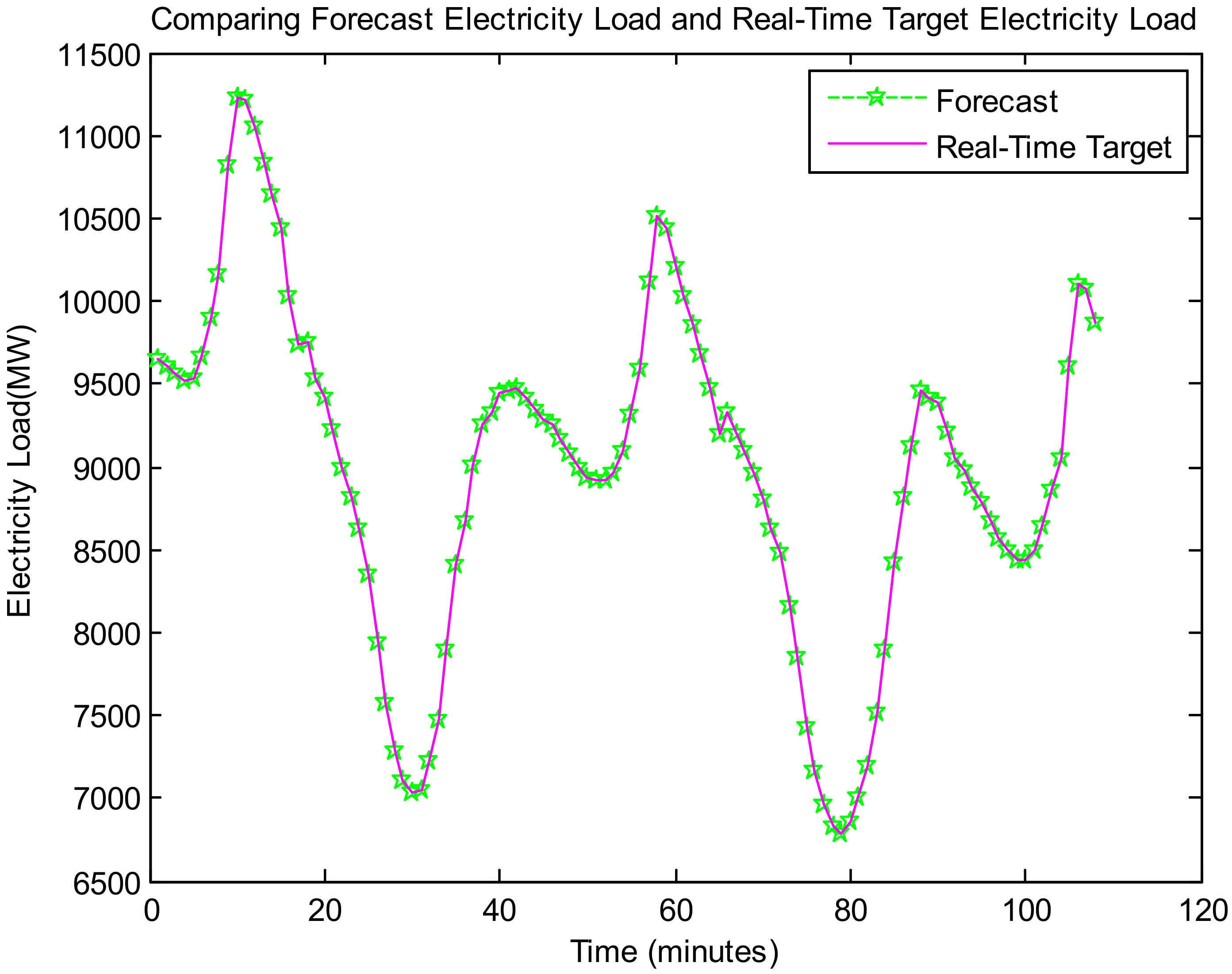
 Figure 26, Figure 27 and Figure 28 represents the proposed model-based output on Dataset 1, namely, comparing the forecast electricity load with real-time target electricity load in the horizon of 30 min ahead, the forecasting error vs. time, and the relationship between real-time target and forecast electricity load for the very short-term time horizons, respectively (Dataset 1). Figure 29, Figure 30 and Figure 31 show the results of very short-term load forecasting concern on Dataset 1. Figure 29, Figure 30 and Figure 31 represent the proposed model-based output on Dataset 2, namely, comparing the forecast electricity load with real-time electricity load in the horizon of 30 min ahead, forecasting error vs. time, and the relationship between real-time target and forecast electricity load for the very short-term time horizons, respectively (Dataset 2).
Figure 8, Figure 14, Figure 20, and Figure 26 show that the output results concerned to Dataset 1 (forecast electricity load) exactly match the target real-time electricity load for different forecasting horizons. Therefore, the forecasting errors are minimal, inferred from Figure 9, Figure 15, Figure 21, and Figure 27. The relationship between real-time target and forecast electricity load is linear, understood clearly from Figure 10, Figure 16, Figure 22, and Figure 28. Similarly, Figure 11, Figure 17, Figure 23, and Figure 29 show that the output results concerned to Dataset 2 (forecast electricity load) exactly match the target real-time electricity load for different forecasting horizons. Therefore, the forecasting errors are minimal, inferred from Figure 12, Figure 18, Figure 24, and Figure 30. The relationship between real-time target and forecast electricity load is linear, understood clearly from Figure 13, Figure 19, Figure 25, and Figure 31.
To better understand the proposed model’s effectiveness regarding different forecasting horizons, the graphical representation of the proposed model performance investigation is based on the different forecasting horizons depicted in Figure 32 (Dataset 1) and Figure 33 (Dataset 2).
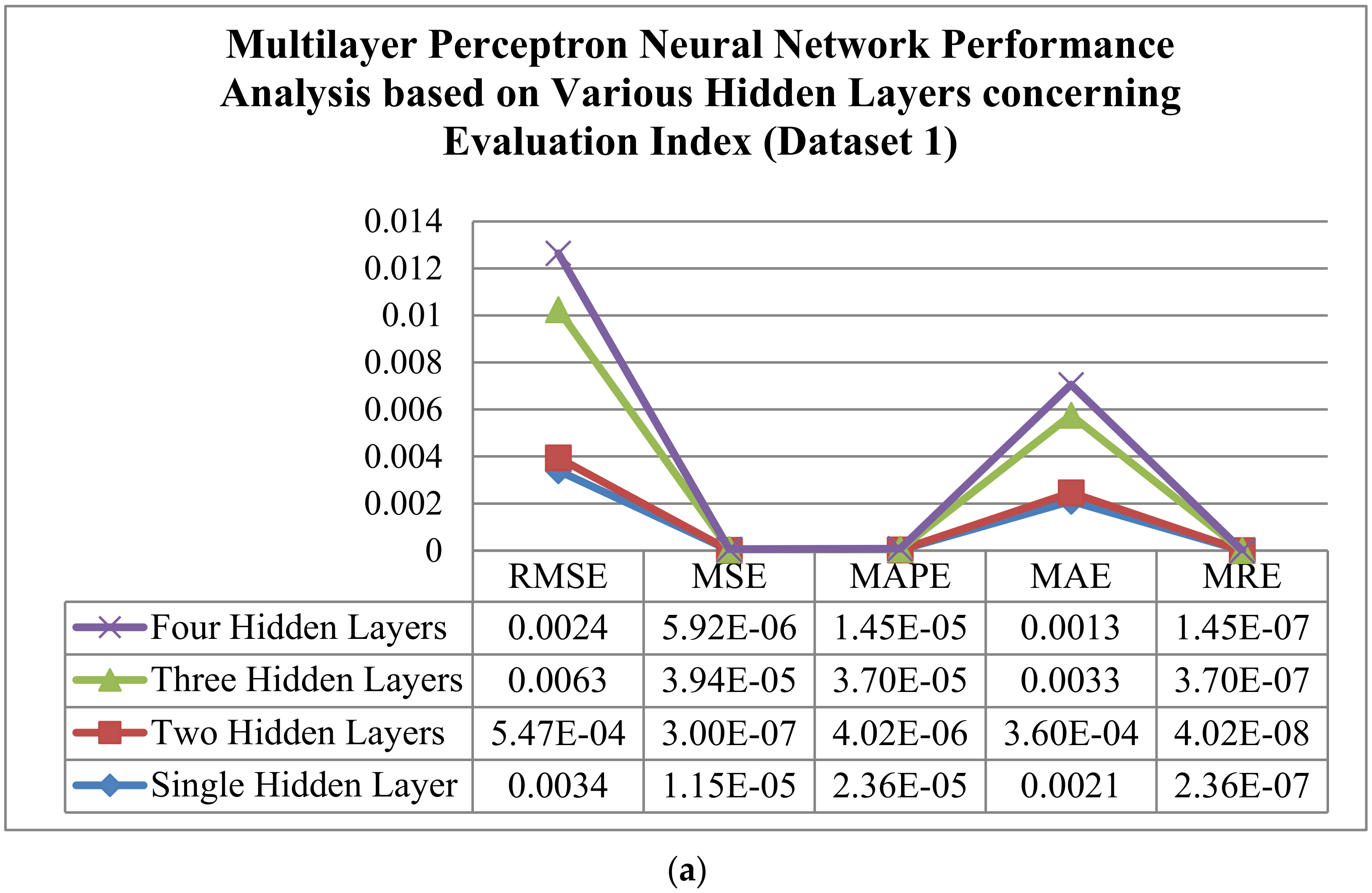
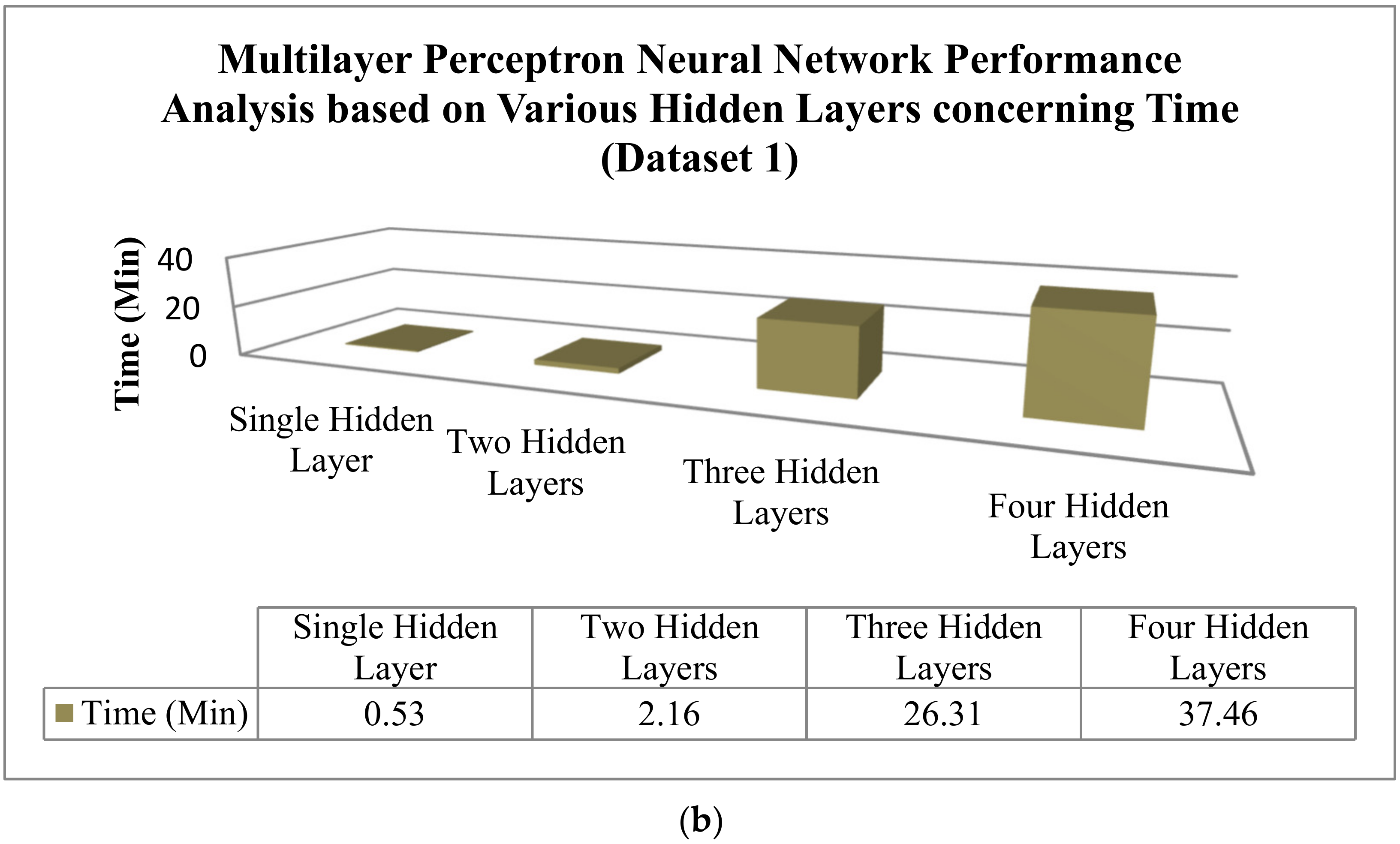
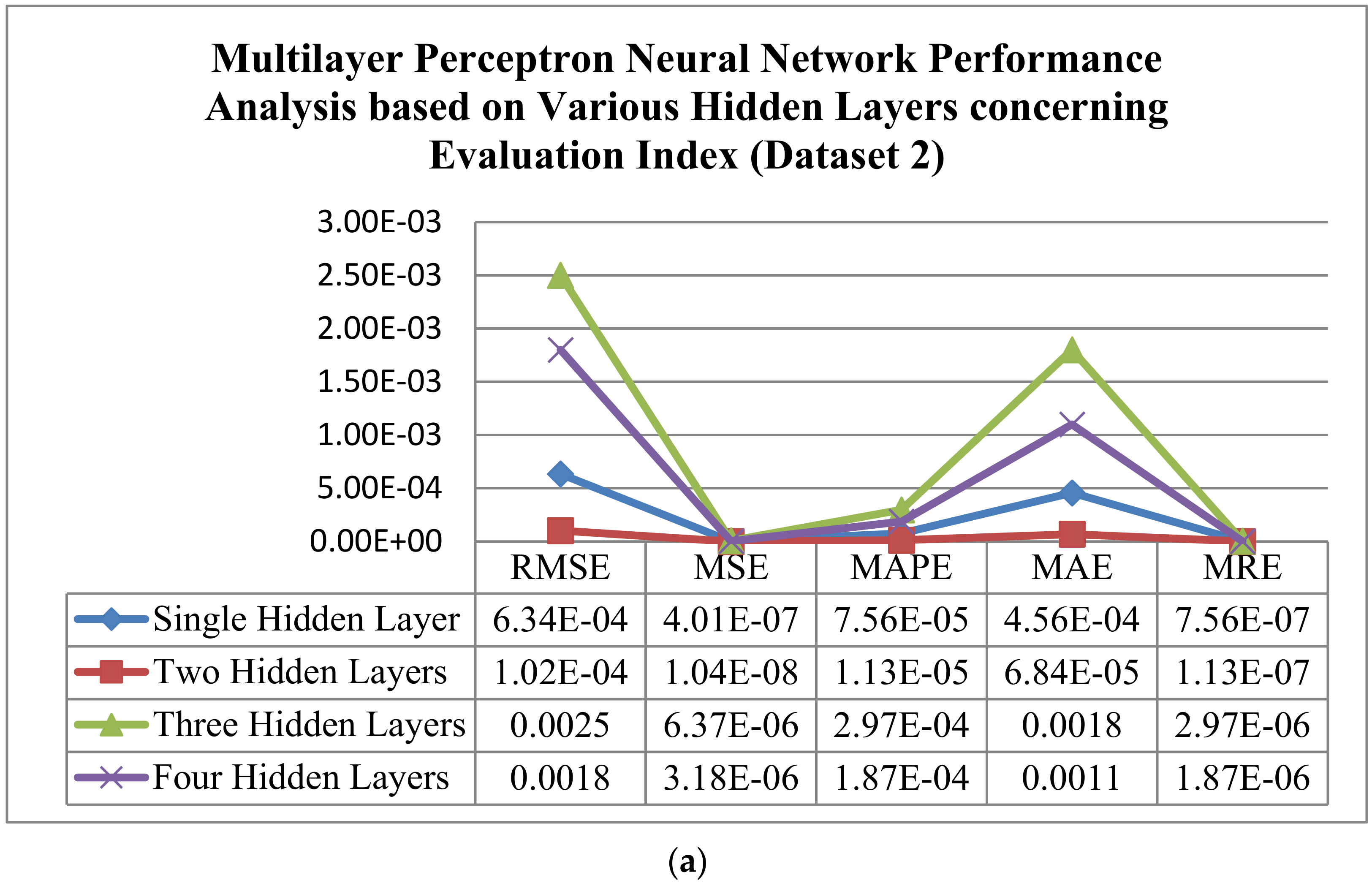
The authors carried out performance analysis with various hidden layers, namely, single hidden layer, two hidden layers, three hidden layers, and four hidden layers based on the obtained results are tabulated in Table 9 and Table 10, respectively, for Dataset 1 and Dataset 2. According to the universal approximation theorem [28,29], the multilayer perceptron neural network with two hidden layers can solve any problem. If the number of hidden layers is increased by more than two, it may cause an issue with respect to convergence and learning. From Figure 34a,b and Figure 35a,b, and Table 9 and Table 10, it is noticed that the results of the two hidden layer-based developed models perform well with improved accuracy.
To further analyze the performance, in addition to the above considered six inputs, the time-series data (holiday) was included as one of the proposed model’s inputs. The obtained results based on structure (1-17-1), one input layer with seven inputs, a single hidden layer with 17 hidden neurons, and one output layer for two datasets are tabulated in Table 11. From Table 11, it is noticed that the load forecasting model performance improved considering the time series as one of the inputs to the forecasting model. It perceives the importance of time series data on load forecasting.
The issues due to uncertainty in electricity load can be resolved by electricity load forecasting. Various electricity load forecasting models have endeavored during the past two decades, but a simple, faster, and highly accurate forecasting model is the thrust field in electricity load forecasting. Therefore, this paper proposed a multilayer perceptron neural network-based exact forecast for electricity forecasting required for the utility system’s effective operation.
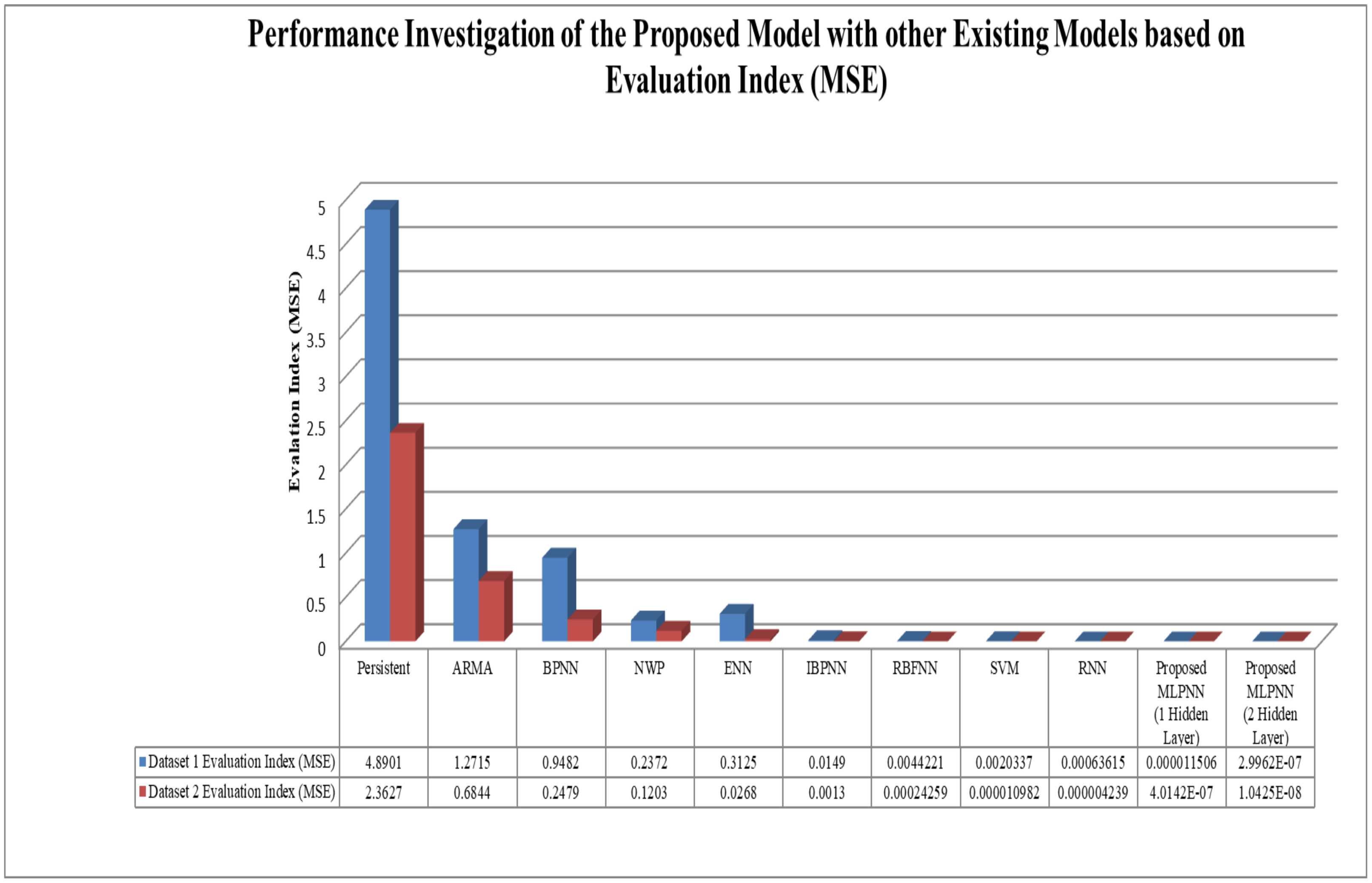
The proposed model’s performance is further investigated against other existing models that concern long-term electricity load forecasting. The corresponding outputs are based on the proposed model and other existing models reported in Table 12. For comparative analysis, we use the existing model’s setting parameters as mentioned by the respective authors, and we performed an evaluation on the considered two datasets. The results were compared with previous models such as persistence, autoregression moving average, backpropagation neural network, numerical weather prediction, Elman neural network, improved back propagation neural network, radial basis function neural network, support vector machine, and recurrent neural network, comparative analysis proves the significance of the proposed model.
Table 12 infers that the proposed model-based results demonstrate superior performance and minimal evaluation index mean square error (MSE) of 1.1506 × 10−05 for Dataset 1 and MSE of 4.0142 × 10−07 for Dataset 2 with concern to the single hidden layer and MSE of 2.9962 × 10−07 for Dataset 1, and MSE of 1.0425 × 10−08 for Dataset 2 concern the two hidden-layers based proposed model than the considered existing models. For a better understanding, the graphical representation of the proposed model’s performance investigation with other existing models is shown in Figure 36. The presented model-based forecasting simulation results indicate the superiority and outperforming capability that of the existing models.

4. Conclusions

The developing countries’ growth regarding the industrial enhancement of any country’s electricity is a driving force to decide the development and economy. To ensure effective planning and achieve better energy system operation, accurate electricity load forecasting receives a center of attention. Electricity load forecasting with the lowest error value is a requisite to perform a better reliable power system working.
The improper planning of power systems concerning the electricity load causes issues as follows:
  • Grid Collapse Issue.
  • Power Outage Issue.
  • Power Stability Issue.
  • Power Quality Issue.
  • Security and Safety Issues.
  • Power Interruption Issue.
A highly desirable way to reduce the above-said problems is to model a simple, faster, and high accurate electricity load forecasting model. The precise load forecasting model leverages economic loss minimization, reduces the grid operating expenses, and improves power quality and continuous power provision to the consumer. Therefore, this work presents a multilayer perceptron neural network-based different forecasting horizons for electricity load forecasting.
This paper summarizes in key points as follows:
  • Perform the proposed model design implementation;
  • Analysis of the hidden neurons’ impact on the proposed forecasting model and identified 17 numbers of hidden neurons as the optimal hidden neurons of the proposed model through the lowest error indexes;
  • The identified hidden neurons-based proposed forecasting model performance was further analyzed concerning various time horizon-based electricity load forecasting and performance assessed employing the error indexes. In all time horizons, the proposed model-based simulation results in a good forecast with minimal forecasting errors;
  • Finally, a performance investigation is performed with respect to various hidden layers and the inclusion of time series data (holiday) as one of the inputs. Perform a comparative analysis with other existing model concerns on electricity load forecasting on two datasets, which substantiates the proposed model’s better performance ability than other existing forecasting model concerns for long-term forecasting. Hence, the proposed multilayer perceptron neural network with recursive fine-tuning strategy-based forecasting model confirms the validity on two datasets with much the lowest forecasting error.

Author Contributions

Conceptualization, M.M.; methodology, M.M.; software, M.M.; validation, M.M.; formal analysis, M.M.; investigation, M.M. and M.L.; resources, M.M.; data curation, M.M.; writing—original draft preparation, M.M.; writing—review and editing, M.M. and M.L.; visualization, M.M. and M.L.; supervision, M.M., and M.L.; project administration, M.M.; funding acquisition, M.L. All authors have read and agreed to the published version of the manuscript.

Funding

This research received no external funding.

Institutional Review Board Statement

Not applicable.

Informed Consent Statement

Not applicable.

Data Availability Statement

The data are available upon request.

Acknowledgments

The authors wish to address our thanks to ERCOT (Electric Reliability Council of Texas), the Open Power System Data platform, and the National Oceanic and Atmospheric Administration, United States, for providing a dataset to conduct a simulation.

Conflicts of Interest

The authors declare no conflict of interest.

Glossary

EpochAll the training data pass through this ultimately.
VectorData structure with two components at least.
NeuronNeural network fundamental information processing element.
PerceptronNeuron that takes binary inputs and results in a single binary output.
Activation FunctionVia a nonlinear function, map the input to the output.
TanhS-shaped curve activation function between a −1 and 1 range.
WeightCarries the information about the input pass to the next layer.
BiasUsed for shifting the decision boundary
InitializationThe initial weights and biases of the neural network are used to compute each neuron’s outputs.
Learning RateSpeed of the neural network for each iteration modifies the weights and bias.
LayersNeural network computation stages such as input, hidden, and output.
Input LayerAll input information represents an input feature; this is the first layer that does not have bias.
Hidden LayerLayer between the input and output layers that contains the number of hidden neurons.
Output LayerThe network last layer uses an activation function to produce output; the task determines the number of neurons in this layer.
Multilayer PerceptronOrganized into layers that contain many perceptrons.

References

  1. Staffell, I.; Pfenninger, S. The increasing impact of weather on electricity supply and demand. Energy 2018, 145, 65–78. [Google Scholar] [CrossRef]
  2. Hippert, H.S.; Pedreira, C.E.; Souza, R.C. Neural networks for short-term load forecasting: A review and evaluation. IEEE Trans. Power Syst. 2001, 16, 44–55. [Google Scholar] [CrossRef]
  3. Weron, R. Modeling and Forecasting Electricity Loads and Prices: A Statistical Approach; Wiley: New York, NY, USA, 2006. [Google Scholar]
  4. Hong, T.; Fan, S. Probabilistic electric load forecasting: A tutorial review. Int. J. Forecast. 2016, 32, 914–938. [Google Scholar] [CrossRef]
  5. Wang, P.; Liu, B.; Hong, T. Electric load forecasting with recency effect: A big data approach. Int. J. Forecast. 2016, 32, 585–597. [Google Scholar] [CrossRef] [Green Version]
  6. Alzubi, O.A.; Alzubi, J.A.; Alweshah, M.; Qiqieh, I.; Al-Shami, S.; Ramachandran, M. An Optimal Pruning Algorithm of Classifier Ensembles: Dynamic Programming Approach. Neural Comput. Appl. 2020, 32, 16091–16107. [Google Scholar] [CrossRef]
  7. Momoh, J.A.; Wang, Y.; Elfayoumy, M. Artificial neural network based load forecasting. In Proceedings of the IEEE International Conference on Systems, Man, and Cybernetics, Orlando, FL, USA, 12–15 October 1997; Volume 4, pp. 3443–3451. [Google Scholar]
  8. Erkmen, I.; Topalli, A.K. Four methods for short-term load forecasting using the benefits of artificial intelligence. Electr. Eng. 2003, 85, 229–233. [Google Scholar] [CrossRef]
  9. López, M.; Valero, S.; Sans, C.; Senabre, C.; Gabaldón, A. Comparison of Short-Term Load Forecasting Performance by Neural Network and Autoregressive Based Models. In Proceedings of the 15th International Conference on the European Energy Market (EEM), Lodz, Poland, 27–29 June 2018; pp. 1–5. [Google Scholar] [CrossRef]
  10. Cristian, V.; Iosif, S.; Ioan, F.; Gabriela, P. Short term electric load forecast with artificial neural networks. IFAC Proc. Vol. 2007, 40, 443–449. [Google Scholar] [CrossRef] [Green Version]
  11. Rodrigues, F.; Cardeira, C.; Calado, J.M.F. The daily and hourly energy consumption and load forecasting using artificial neural network method: A case study using a set of 93 households in Portugal. Energy Procedia 2014, 62, 220–229. [Google Scholar] [CrossRef] [Green Version]
  12. Xia, C.; Wang, J.; McMenemy, K. Short, medium and long term load forecasting model and virtual load forecaster based on radial basis function neural networks. Int. J. Electr. Power Energy Syst. 2010, 32, 743–750. [Google Scholar] [CrossRef] [Green Version]
  13. Topalli, A.K.; Erkmen, I.; Topalli, I. Intelligent short-term load forecasting in Turkey. Int. J. Electr. Power Energy Syst. 2006, 28, 437–447. [Google Scholar] [CrossRef]
  14. Senjyu, T.; Takara, H.; Uezato, K.; Funabashi, T. One-Hour-Ahead Load Forecasting Using Neural Network. IEEE Trans. Power Syst. 2002, 17, 113–118. [Google Scholar] [CrossRef]
  15. Zhang, B.; Wu, J.; Chang, P. A multiple time series-based recurrent neural network for short-term load forecasting. Soft Comput. 2018, 22, 4099–4112. [Google Scholar] [CrossRef]
  16. Luo, J.; Hong, T.; Yue, M. Real-time anomaly detection for very short-term load forecasting. J. Mod. Power Syst. Clean Energy 2018, 6, 235–243. [Google Scholar] [CrossRef] [Green Version]
  17. Li, Y.; Han, D.; Yan, Z. Long-term system load forecasting based on data-driven linear clustering method. J. Mod. Power Syst. Clean Energy 2018, 6, 306–316. [Google Scholar] [CrossRef]
  18. Xie, J.; Hong, T. Load forecasting using 24 solar terms. J. Mod. Power Syst. Clean Energy 2018, 6, 208–214. [Google Scholar] [CrossRef] [Green Version]
  19. Santos, P.J.; Martins, A.G.; Pires, A.J. Designing the input vector to ANN-based models for short-term load forecast in electricity distribution systems. Int. J. Electr. Power Energy Syst. 2007, 29, 338–347. [Google Scholar] [CrossRef] [Green Version]
  20. Madhiarasan, M.; Deepa, S.N. Comparative Analysis on Hidden Neurons Estimation in Multi-Layer Perceptron Neural Networks for Wind Speed Forecasting. Artif. Intell. Rev. 2017, 48, 449–471. [Google Scholar] [CrossRef]
  21. Madhiarasan, M.; Tipaldi, M.; Siano, P. Analysis of Artificial Neural Network Performance Based on Influencing Factors for Temperature Forecasting Applications. J. High-Speed Netw. 2020, 26, 209–223. [Google Scholar] [CrossRef]
  22. Madhiarasan, M.; Deepa, S.N. Performance Investigation of Six Artificial Neural Networks for Different Time Scale Wind Speed Forecasting in Three Wind Farms of Coimbatore Region. Int. J. Innov. Sci. Res. 2016, 23, 380–411. [Google Scholar]
  23. Madhiarasan, M.; Deepa, S.N. A Novel Criterion to Select Hidden Neuron Numbers in Improved Back Propagation Networks for Wind Speed Forecasting. Appl. Intell. 2016, 44, 878–893. [Google Scholar] [CrossRef]
  24. Madhiarasan, M.; Deepa, S.N. New Criteria for Estimating the Hidden Layer Neuron Numbers for Recursive Radial Basis Function Networks and Its Application in Wind Speed Forecasting. Asian J. Inf. Technol. 2016, 15, 4377–4391. [Google Scholar]
  25. Madhiarasan, M.; Deepa, S.N. A Novel Method to Select Hidden Neurons in ELMAN Neural Network for Wind Speed Prediction Application. WSEAS Trans. Power Syst. 2018, 13, 13–30. [Google Scholar]
  26. Madhiarasan, M.; Deepa, S.N. Precisious Estimation of Solar Irradiance by Innovative Neural Network and Identify Exact Hidden Layer Nodes through Novel Deciding Standard. Asian J. Res. Soc. Sci. Humanit. 2016, 6, 951–974. [Google Scholar] [CrossRef]
  27. Madhiarasan, M. Long-Term Wind Speed Prediction using Artificial Neural Network-Based Approaches. AIMS Geosci. 2021, 7, 542–552. [Google Scholar] [CrossRef]
  28. Hornik, K.; Stinchcombe, M.; White, H. Multilayer feedforward networks are universal approximators. Neural Netw. 1989, 2, 359–366. [Google Scholar] [CrossRef]
  29. Trenn, S. Multilayer perceptrons: Approximation order and necessary number of hidden units. IEEE Trans. Neural Netw. 2008, 19, 836–844. [Google Scholar] [CrossRef] [Green Version]
  30. Dutta, S.; Li, Y.; Venkataraman, A.; Costa, L.M.; Jiang, T.; Plana, R.; Tordjman, P.; Choo, F.H.; Foo, C.F.; Puttgen, H.B. Load and renewable energy forecasting for a microgrid using persistence technique. Energy Procedia 2017, 143, 617–622. [Google Scholar] [CrossRef]
  31. Pappas, S.S.; Ekonomou, L.; Karamousantas, D.C.; Chatzarakis, G.E.; Katsikas, S.K.; Liatsis, P. Electricity demand loads modeling using AutoRegressive Moving Average (ARMA) models. Energy 2008, 33, 1353–1360. [Google Scholar] [CrossRef]
  32. Lu, Q.; Cai, Q.; Liu, S.; Yang, Y.; Yan, B.; Wang, Y.; Zhou, X. Short-term load forecasting based on load decomposition and numerical weather forecast. In Proceedings of the IEEE Conference on Energy Internet and Energy System Integration (EI2), Beijing, China, 26–28 November 2017; pp. 1–5. [Google Scholar]
  33. Hong, W.-C. Electric load forecasting by support vector model. Appl. Math. Model. 2009, 33, 2444–2454. [Google Scholar] [CrossRef]
Figure 1. Implementation structural flow of the proposed model.
Forecasting 03 00049 g001
Figure 2. (a). Collected Dataset 1—real-time electricity load data concerning time. (b). Collected Dataset 2—real-time electricity load data concerning time.
Forecasting 03 00049 g002
Figure 3. The architecture of the proposed multilayer perceptron neural network-based electricity load forecasting model.
Forecasting 03 00049 g003
Figure 4. Proposed MLPNN Performance Investigation based on Hidden Neurons (Dataset 1).
Forecasting 03 00049 g004
Figure 5. Proposed MLPNN Performance Investigation based on Hidden Neurons (Dataset 2).
Forecasting 03 00049 g005
Figure 6. Comparison of Real-Time Target and Forecast Electricity Load (Dataset 1).
Forecasting 03 00049 g006
Figure 7. Comparison of Real-Time Target and Forecast Electricity Load (Dataset 2).
Forecasting 03 00049 g007
Figure 8. Comparing the forecast electricity load and real-time target electricity load for a long-term horizon (Dataset 1).
Forecasting 03 00049 g008
Figure 9. Forecasting error vs. time for a long-term horizon (Dataset 1).
Forecasting 03 00049 g009
Figure 10. Relationship between real-time target and forecast electricity load for a long-term horizon (Dataset 1).
Forecasting 03 00049 g010
Figure 11. Comparing the forecast electricity load and real-time target electricity load for a long-term horizon (Dataset 2).
Forecasting 03 00049 g011
Figure 12. Forecasting error vs. time for a long-term horizon (Dataset 2).
Forecasting 03 00049 g012
Figure 13. Relationship between real-time target and forecast electricity load for a long-term horizon (Dataset 2).
Forecasting 03 00049 g013
Figure 14. Comparing the forecast electricity load and real-time target electricity load for a medium-term horizon (Dataset 1).
Forecasting 03 00049 g014
Figure 15. Forecasting error vs. time for a medium-term horizon (Dataset 1).
Forecasting 03 00049 g015
Figure 16. Relationship between real-time target and forecast electricity load for a medium-term horizon (Dataset 1).
Forecasting 03 00049 g016
Figure 17. Comparing the forecast electricity load and real-time target electricity load for a medium-term horizon (Dataset 2).
Forecasting 03 00049 g017
Figure 18. Forecasting error vs. time for a medium-term horizon (Dataset 2).
Forecasting 03 00049 g018
Figure 19. Relationship between real-time target and forecast electricity load for a medium-term horizon (Dataset 2).
Forecasting 03 00049 g019
Figure 20. Comparing the forecast electricity load and real-time target electricity load for a short-term horizon (Dataset 1).
Forecasting 03 00049 g020
Figure 21. Forecasting error vs. time for a short-term horizon (Dataset 1).
Forecasting 03 00049 g021
Figure 22. Relationship between real-time target and forecast electricity load for a short-term horizon (Dataset 1).
Forecasting 03 00049 g022
Figure 23. Comparing the forecast electricity load and real-time target electricity load for a short-term horizon (Dataset 2).
Forecasting 03 00049 g023
Figure 24. Forecasting error vs. time for a short-term horizon (Dataset 2).
Forecasting 03 00049 g024
Figure 25. Relationship between real-time target and forecast electricity load for a short-term horizon (Dataset 2).
Forecasting 03 00049 g025
Figure 26. Comparing the forecast electricity load and real-time target electricity load for a very short-term horizon (Dataset 1).
Forecasting 03 00049 g026
Figure 27. Forecasting error vs. time for a very short-term horizon (Dataset 1).
Forecasting 03 00049 g027
Figure 28. Relationship between real-time target and forecast electricity load for a very short-term horizon (Dataset 1).
Forecasting 03 00049 g028
Figure 29. Comparing the forecast electricity load and real-time target electricity load for a very short-term horizon (Dataset 2).
Forecasting 03 00049 g029
Figure 30. Forecasting error vs. time for a very short-term horizon (Dataset 2).
Forecasting 03 00049 g030
Figure 31. Relationship between real-time target and forecast electricity load for a very short-term horizon (Dataset 2).
Forecasting 03 00049 g031
Figure 32. Proposed model performance investigation based on different forecasting horizons (the proposed load forecasting model proves validity for different forecasting horizons) (Dataset 1).
Forecasting 03 00049 g032
Figure 33. Proposed model performance investigation based on different forecasting horizons (the proposed load forecasting model proves validity for different forecasting horizons) (Dataset 2).
Forecasting 03 00049 g033
Figure 34. (a) Proposed Multilayer Perceptron Neural Network Performance Analysis based on Various Hidden Layers concerning Evaluation Index (Dataset 1), (b) Proposed Multilayer Perceptron Neural Network Performance Analysis based on Various Hidden Layers concerning Time (Dataset 1).
Forecasting 03 00049 g034aForecasting 03 00049 g034b
Figure 35. (a) Proposed Multilayer Perceptron Neural Network Performance Analysis based on Various Hidden Layers concerning Evaluation Index (Dataset 2), (b) Proposed Multilayer Perceptron Neural Network Performance Analysis based on Various Hidden Layers concerning Time (Dataset 2).
Forecasting 03 00049 g035aForecasting 03 00049 g035b
Figure 36. Performance Investigation of the Proposed Model with other Existing Models (the Proposed Model Achieves Minimal MSE than Other Models).
Forecasting 03 00049 g036
Table 1. Proposed multilayer perceptron neural network implementation parameters.
MLPNNVariable
Input neurons6 inputs
Number of hidden layers1
Output neuron1
Number of epochs100
Threshold1
Learning rate0.9
Table 2. Mathematical modeling of the proposed neural network variables.
VariablesMathematical Model
V 1 , V 2 , V 3 , V 4 , V 5 , V 6 : U Electricity Load, Temperature, Humidity, Wind speed, Solar Irradiance, and Pressure: Forecast Electricity Load
Input vector V = E L , T , H , W S , S I , P
Output vector U = E L f
Weight vector of input to hidden vector V H w = V H w 11 , V H w 12 , , V H w 1 n , V H w 21 , V H w 22 , , V H w 2 n , V H w 31 , V H w 32 , , V H w 3 n , V H w 41 , V H w 42 , , V H w 4 n , V H w 51 , V H w 52 , , V H w 5 n , V H w 61 , V H w 62 , V H w 6 n
Net input of the hidden layer S i n q = p = 1 6 q = 1 n V p V H w p q
The output of the hidden layer S q = f p = 1 6 q = 1 n V p V H w p q
Weight vector of the hidden to output vector H U w = H U w 1 , H U w 2 , , H U w n
Net input of the output layer U i n = q = 1 n S q H U w q
Output U = f q = 1 n S q H U w q , q = 1 , 2 , , n
Table 3. Proposed Multilayer Perceptron Neural Network Performance Investigation based on Hidden Neurons (Dataset 1). The best result highlighted in bold.
Number of Hidden NeuronsRRMSE (MW)MSE (MW)MAPE (%)MAE (MW)MRE (MW)Time (Min)
110.06110.00373.9780 × 10−040.03453.9780 × 10−063.40
210.11230.01266.5644 × 10−040.05696.5644 × 10−064.16
310.04150.00172.4281 × 10−040.02102.4281 × 10−062.28
410.03500.00122.0209 × 10−040.01752.0209 × 10−063.21
510.04150.00172.2467 × 10−040.01952.2467 × 10−062.53
610.06830.00472.8929 × 10−040.02512.8929 × 10−064.07
710.18140.03297.2299 × 10−040.06277.2299 × 10−061.20
810.09930.00995.7910 × 10−040.05025.7910 × 10−062.58
910.08770.00773.0617 × 10−040.02653.0617 × 10−061.42
1010.01101.2147 × 10−044.6222 × 10−050.00404.6222 × 10−071.23
1110.12990.01692.6603 × 10−040.02312.6603 × 10−064.36
1210.17270.02982.8220 × 10−040.02452.8220 × 10−063.32
1310.02234.9842 × 10−049.4412 × 10−040.00829.4412 × 10−061.14
1410.05060.00261.2202 × 10−040.01061.2202 × 10−061.14
1510.00826.7078 × 10−053.1766 × 10−050.00283.1766 × 10−072.10
1610.01863.4761 × 10−043.6966 × 10−050.00323.6966 × 10−071.35
1710.00341.1506 × 10−052.3633 × 10−050.00212.3633 × 10−070.53
1810.00411.6756 × 10−053.1653 × 10−050.00273.1653 × 10−072.53
1910.37290.13912.3504 × 10−040.02642.3504 × 10−067.57
2010.01542.3689 × 10−045.0313 × 10−050.00585.0313 × 10−071.30
2110.52020.27062.5002 × 10−040.02172.5002 × 10−061.51
2210.11390.01306.9052 × 10−050.00606.9052 × 10−071.13
2310.16000.02567.1411 × 10−050.00627.1411 × 10−071.02
2410.49830.24832.2323 × 10−040.01932.2323 × 10−061.15
2510.60280.36332.6556 × 10−040.02302.6556 × 10−061.19
2611.05181.10625.1499 × 10−040.04465.1499 × 10−061.40
2711.79563.22437.9421 × 10−040.06887.9421 × 10−062.48
2811.89953.60798.2907 × 10−040.07198.2907 × 10−063.15
2912.11054.45429.3820 × 10−040.08139.3820 × 10−062.13
3012.16744.69750.00100.08871.0238 × 10−051.41
Table 4. Proposed Multilayer Perceptron Neural Network Performance Investigation based on Hidden Neurons (Dataset 2). The best result highlighted in bold.
Number of Hidden NeuronsRRMSE (MW)MSE (MW)MAPE (%)MAE (MW)MRE (MW)Time (Min)
110.00361.2624 × 10−053.4874 × 10−040.00213.4874 × 10−063.29
210.00573.2881 × 10−056.1681 × 10−040.00376.1681 × 10−062.22
310.00193.7200 × 10−062.0454 × 10−040.00122.0454 × 10−061.24
410.00472.1769 × 10−052.1105 × 10−040.00135.1105 × 10−061.12
518.0651 × 10−046.5047 × 10−077.9919 × 10−054.8235 × 10−047.9919 × 10−070.50
610.00694.7877 × 10−056.9094 × 10−040.00426.9094 × 10−060.52
710.00603.6134 × 10−056.8661 × 10−040.00416.8661 × 10−061.01
810.01291.6665 × 10−048.6983 × 10−040.00528.6983 × 10−061.40
910.01191.4146 × 10−047.6589 × 10−040.00467.6589 × 10−061.12
1010.00321.0426 × 10−051.5744 × 10−049.5022 × 10−041.5744 × 10−061.53
1110.02245.0346 × 10−042.3288 × 10−040.00142.3288 × 10−060.58
1210.02034.1312 × 10−044.9893 × 10−040.00304.9893 × 10−062.36
1310.01502.2623 × 10−042.0179 × 10−040.00122.0179 × 10−063.25
1410.02194.8096 × 10−043.6904 × 10−040.00223.3904 × 10−065.33
1510.00887.7729 × 10−051.2778 × 10−047.7123 × 10−041.2778 × 10−063.02
1610.00152.3690 × 10−069.3744 × 10−058.2954 × 10−049.3744 × 10−071.39
1716.3358 × 10−044.0142 × 10−077.5578 × 10−054.5615 × 10−047.5578 × 10−070.34
1810.04640.00225.1669 × 10−040.00315.1669 × 10−063.27
1910.00173.0617 × 10−069.7188 × 10−058.5399 × 10−049.7188 × 10−072.59
2010.00502.4763 × 10−053.0130 × 10−049.8185 × 10−043.0130 × 10−060.56
2110.01251.5509 × 10−043.4901 × 10−040.00213.4901 × 10−061.08
2210.00287.5683 × 10−061.2190 × 10−049.3573 × 10−041.2190 × 10−061.31
2310.01371.8660 × 10−041.2801 × 10−040.00131.2801 × 10−061.09
2410.06930.00483.2042 × 10−040.00193.2045 × 10−063.24
2510.05500.00302.5498 × 10−040.00152.5498 × 10−063.07
2610.10150.01035.4809 × 10−040.00335.4809 × 10−064.13
2710.08530.00733.8967 × 10−040.00243.8967 × 10−063.15
2810.09640.00937.0402 × 10−040.00427.0402 × 10−062.04
2910.08800.00774.4857 × 10−040.00274.4857 × 10−061.30
3010.02797.7623 × 10−045.2729 × 10−040.00375.2729 × 10−061.32
Table 5. Comparison of Real-Time Target and Forecast Electricity Load (Dataset 1).
Real-Time Target Electricity Load (MW)Forecast Electricity Load (MW)Time Stamp (Min)Real-Time Target Electricity Load (MW)Forecast Electricity Load (MW)Time Stamp (Min)
7907.31127907.31309682.04809682.05450
8334.42808334.43609589.14969589.15480
8747.04218747.04909362.00179362510
9068.74799068.751209084.80799084.81540
9104.62819104.631508849.60058849.6570
9169.84889169.851808654.60238654.6600
9129.68839129.692108576.97148576.97630
8985.06828985.072408413.97858413.98660
8878.61008878.612708218.84938218.85690
8775.48188775.483008289.35838289.36720
8678.08248678.083308225.95928225.96750
8540.01088540.013608170.33038170.33780
8431.25878431.263907973.18237973.18810
8347.81808347.824207738.80767738.81840
Table 6. Comparison of Real-Time Target and Forecast Electricity Load (Dataset 2).
Real-Time Target Electricity Load (MW)Forecast Electricity Load (MW)Time Stamp (Min)Real-Time Target Electricity Load (MW)Forecast Electricity Load (MW)Time Stamp (Min)
618617.999430441441.0008450
604603.999560455455.0002480
619618.999490508507.9997510
636635.9994120534534.0003540
630629.9993150556556.0004570
615614.9994180582582600
607606.9995210565565.0003630
599598.9996240568568.0003660
596595.9997270564564.0003690
607606.9995300536536.0003720
686686.0004330552552.0004750
640639.9994360553553.0004780
534534.0003390542542.0004810
491490.9993420542542.0004840
Table 7. Multilayer Perceptron Neural Network Performance Analysis based on Different Forecasting Horizons (Dataset 1).
Forecasting HorizonsRRMSE (MW)MSE (MW)MAPE (%)MAE (MW)MRE (MW)Time (Min)
Long-Term Forecasting10.00341.1506 × 10−052.3633 × 10−050.00212.3633 × 10−070.53
Medium-Term Forecasting10.00552.9774 × 10−052.2685 × 10−050.00192.2685 × 10−070.32
Short-Term Forecasting10.03170.00107.8244 × 10−050.00707.8244 × 10−070.14
Very Short-Term Forecasting10.15850.02510.00150.13461.5219 × 10−050.05
Table 8. Multilayer Perceptron Neural Network Performance Analysis based on Different Forecasting Horizons (Dataset 2).
Forecasting HorizonsRRMSE (MW)MSE (MW)MAPE (%)MAE (MW)MRE (MW)Time (Min)
Long-Term Forecasting16.3358 × 10−044.0142 × 10−077.5578 × 10−054.5615 × 10−047.5578 × 10−070.34
Medium-Term Forecasting10.00583.3713 × 10−052.5651 × 10−040.00192.5651 × 10−060.20
Short-Term Forecasting10.01542.3704 × 10−049.1914 × 10−040.00609.1914 × 10−060.07
Very Short-Term Forecasting10.01552.4112 × 10−040.00200.01232.0396 × 10−050.04
Table 9. Multilayer Perceptron Neural Network Performance Analysis based on Various Hidden Layers (Dataset 1). The best result highlighted in bold.
MLPN with Various
Hidden Layer
RRMSE (MW)MSE (MW)MAPE (%)MAE (MW)MRE (MW)Time (Min)
Single Hidden Layer10.00341.1506 × 10−052.3633 × 10−050.00212.3633 × 10−070.53
Two Hidden Layers15.4737 × 10−042.9962 × 10−074.0204 × 10−063.6012 × 10−044.0204 × 10−082.16
Three Hidden Layers10.00633.9356 × 10−053.7044 × 10−050.00333.7044 × 10−0726.31
Four Hidden Layers10.00245.9191 × 10−061.4484 × 10−050.00131.4484 × 10−0737.46
Table 10. Multilayer Perceptron Neural Network Performance Analysis based on Various Hidden Layers (Dataset 2). The best result highlighted in bold.
MLPN with Various
Hidden Layer
RRMSE (MW)MSE (MW)MAPE (%)MAE (MW)MRE (MW)Time (Min)
Single Hidden Layer16.3358 × 10−044.0142e-077.5578 × 10−054.5615 × 10−047.5578 × 10−070.34
Two Hidden Layers11.0210 × 10−041.0425 × 10−081.1327 × 10−056.8365 × 10−051.1327 × 10−071.40
Three Hidden Layers10.00256.3659 × 10−062.9744 × 10−040.00182.9744 × 10−0620.55
Four Hidden Layers10.00183.1809 × 10−061.8707 × 10−040.00111.8707 × 10−0632.08
Table 11. Multilayer Perceptron Neural Network Performance Analysis based on Seven Inputs, Including Time-Related Data (Holiday).
MLPN with 7 Inputs (1-17-1)RRMSE (MW)MSE (MW)MAPE (%)MAE (MW)MRE (MW)Time (Min)
Data set 113.3494 × 10−041.1219 × 10−072.4396 × 10−062.1852 × 10−042.4396 × 10−081.28
Dataset 219.1288 × 10−058.3334 × 10−091.0124 × 10−056.1104 × 10−051.0124 × 10−070.59
Table 12. Performance Investigation of the Proposed Model with other Existing Models. The best result highlighted in bold.
S. NoModelsAuthorsDataset 1Dataset 2
Evaluation Index (MSE)Evaluation Index (MSE)
1PersistentDutta, Shreya et al. 2017 [30]4.89012.3627
2Auto-Regressive Moving Average Pappas, S.S. et al. 2008 [31]1.27150.6844
3Back Propagation Neural NetworkMomoh, J.A. et al. 1997 [7]0.94820.2479
4Numerical Weather Prediction Qiuyu, Lu et al. 2017 [32]0.23720.1203
5Elman Neural NetworkVasar Cristian et al. 2007 [10]0.31250.0268
6Improved Back Propagation Neural NetworkMadhiarasan and Deepa S.N. 2016 [23]0.01490.0013
7Radial Basis Function Neural NetworkXia et al. 2010 [12]4.4221 × 10−032.4259 × 10−04
8Support Vector MachineHong, Wei-Chiang 2009 [33]2.0337 × 10−031.0982 × 10−05
9Recurrent Neural NetworkZhang et al. 2018 [15]6.3615 × 10−044.2390 × 10−06
10Proposed Multilayer Perceptron Neural Network (Single Hidden Layer)Madhiarasan and Louzazni 20211.1506 × 10−054.0142 × 10−07
11Proposed Multilayer Perceptron Neural Network (Two Hidden Layer)Madhiarasan and Louzazni 20212.9962 × 10−071.0425 × 10−08
Publisher’s Note: MDPI stays neutral with regard to jurisdictional claims in published maps and institutional affiliations.

