
Hybrid Surrogate Model for Timely Prediction of Flash Flood Inundation Maps Caused by Rapid River Overflow


1
Department of Civil Engineering, McMaster University, 1280 Main Street West, Hamilton, ON L8S 4L7, Canada
2
School of Earth, Environment and Society, McMaster University, 1280 Main Street West, Hamilton, ON L8S 4L7, Canada
3
Institute for Water, Environment, and Health, United Nations University, 175 Longwood Road, Hamilton, ON L8P 0A1, Canada
*
Author to whom correspondence should be addressed.
Forecasting 2022, 4(1), 126-148; https://0-doi-org.brum.beds.ac.uk/10.3390/forecast4010007
Submission received: 15 November 2021
/
Revised: 20 December 2021
/
Accepted: 20 January 2022
/
Published: 23 January 2022
(This article belongs to the Special Issue Innovative Approaches for Environmental and Natural Hazard Forecasting: Proposals from Theory to Practice)
Abstract
:Timely generation of accurate and reliable forecasts of flash flood events is of paramount importance for flood early warning systems in urban areas. Although physically based models are able to provide realistic reproductions of fast-developing inundation maps in high resolutions, the high computational demand of such hydraulic models makes them difficult to be implemented as part of real-time forecasting systems. This paper evaluates the use of a hybrid machine learning approach as a surrogate of a quasi-2D urban flood inundation model developed in PCSWMM for an urban catchment located in Toronto (Ontario, Canada). The capability to replicate the behavior of the hydraulic model was evaluated through multiple performance metrics considering error, bias, correlation, and contingency table analysis. Results indicate that the surrogate system can provide useful forecasts for decision makers by rapidly generating future flood inundation maps comparable to the simulations of physically based models. The experimental tool developed can issue reliable alerts of upcoming inundation depths on traffic locations within one to two hours of lead time, which is sufficient for the adoption of important preventive actions. These promising outcomes were achieved in a deterministic setup and use only past records of precipitation and discharge as input during runtime.
1. Introduction
The World Meteorological Organization estimates that flash floods are responsible for more than 5000 human deaths every year, making them the most frequent and with highest morality rate type of flooding [1]. The continuous densification of urban areas associated with the increasing recurrence of high intensity precipitation driven by climate change has the potential to intensify the frequency of such events [2,3,4]. To mitigate impacts, flash flood early warning systems have been implemented around the world since the 1970s mainly by governmental agencies (e.g., provincial or national flood/flow forecasting centers) [5], and the development of techniques and technologies to improve their predictive performance is an active research topic [6,7]. A pivotal component of such systems is the real-time forecasting of hazardous scenarios, which is decisive for decision makers on the task of choosing whether or not to take actions. Preventive actions such as closing roads, evacuating buildings, and changing the current operation of a dam have the potential to cause significant social disturbance and economical loss, thus a system that issues an excessive number of false alarms is undesired. To be operationally applicable, a forecasting system is expected to produce trustable and timely predictions, especially in the context of flash floods due to their rapid development, which happens “within six hours of the causative event (e.g., intense rainfall, dam failure, ice jam)”, as defined by the United States’ National Weather Service [5].
The capability of forecasting flood inundation maps (IMs) is usually considered a valuable asset to complement the usual river discharge hydrographs due to the direct representation of the locations to be (or not) inundated. As flash floods are characterized by flows with high motion, realistic IMs of such events are attained through the simulation of physically based hydraulic models that solve the two-dimensional (2D) or quasi-2D Saint-Venant equation considering both mass and momentum conservation [8]. However, the computational cost of such models usually becomes a constraint for their direct use as part of toolchains of forecasting systems. One of the strategies developed for obtaining IMs in a time interval compatible to the update cycles of real-time flood forecasting systems is based on the development of simplified 2D models such as the Height Above Nearest Drainage [9], AutoRAPID [10] and Safer_RAIN [11], which adopt the approach of “spilling and filling” digital elevation models at specific water heights. Despite providing realistic results for flood events of large scale with applicability demonstrated in real-time scenarios [12], the lack of physics for representing momentum results in limited applicability for rapidly-evolving flash flood events [13,14]. Other modelling approaches developed for reducing the computational burden of high-resolution models that do not neglect the momentum component include sub-grid techniques [15,16], the use of cellular automata frameworks [17], and the development of new systems and models specifically designed to explore the processing power of graphic processing units [18,19]. The implementation of such promising techniques, however, may require expensive tasks of reimplementing already existing hydrological models using such new tools and the training of the technical team for the use of such frameworks.
In this context, the development of response surface surrogate models (hereafter simply referred to as “surrogate models") have been explored as workarounds to rapidly estimate realistic IMs. Surrogate models are mathematical systems calibrated to map values in the input space to values in the output space of more complex, physically based and computationally expensive simulation systems, thus reproducing their behavior through the use of a simplified set of equations derived from statistical or data-driven approaches [20].
The use of machine learning techniques for the development of surrogate inundation models has presented significant evolution in recent years. Here, a hydraulic model in which both mass and momentum components of the surface water flow are present is implemented for the region of interest. Such a hydraulic model is assumed to be a realistic representation of the environment and is used to simulate the behavior of the system when forced with a wide range of realistic forcing values. The resulting IMs are stored, and a data-driven system is then trained to map each forcing data used to the respective IM produced. The high number of 2D cells in regular IMs to which a water depth value must be estimated, associated with the costly task of generating a large number of simulation products, usually leads to the challenging issue of properly tuning very complex models with limited input/output datasets. A common approach to reduce the number of variables to be predicted by the data-driven method is to train multiple independent simpler networks covering smaller parts of the grid, be it one model trained for each individual grid cell [21] or one model per groups of neighboring grid cells [22]. Such a strategy has as drawbacks: (1) the need to train a potentially extensive number of subnetworks, which can and up being a constraint in operational environments when the hydraulic/hydrological model is continuously updated (thus demanding continuous retraining of the surrogate model); and (2) the fact that the spatial correlation of nearby grids trained by independent predictors is lost, potentially resulting in unrealistic discontinuities in the estimated IM.
In this context, the use of a Self-Organizing Maps (SOM) model was proposed as a dimensionality reduction method by Chang et al. [23] for regional flood inundation forecasting triggered by river overflow. In their work, SOMs are trained to cluster the inundation maps of the training dataset so that the topologic nodes of the network hold what can be interpreted as representative inundation instant conditions of the covered area. The average inundation depth (AID) of each topological node is calculated and stored as an associated variable after the tuning step so that a univariate predicted AID value can be used for querying complete IMs during forecasting time. A recurrent model is then trained to predict the univariate AID variable out of descriptive hydrologic observed features to provide the temporal development of the event. Chang et al. [23] reported promising results for the prediction of inundation maps with spatiotemporal resolution of 75 km/3 h for a lead time of up to 12 h, a configuration suitable for the regional scope evaluated in their work (total area of 100 km2 in the outlet of the nearly 2000 km2 Kemaman River Basin, Malaysia). Kim et al. [24] applied a similar approach on a finer grid resolution and assessed its effectiveness on timely predicting flash flood inundation scenarios caused by direct runoff generation and consequent sewer overflow in a densely occupied urban area in Seoul, South Korea, under heavy rain. In their work, the overflow of 103 manholes were used as the querying variables and 122 rainfall events were applied for training the networks. Consistent results were obtained when the analysis was later extended to 24 districts [25]. Nonlinear Autoregressive neural network with exogenous inputs (NARX) is the recurrent structure commonly chosen by the abovementioned works due to its simplicity and efficiency.
To the best of the author’s knowledge, results for the application of such a hybrid approach are yet to be reported for urban catchments prone to flash flood events caused by fast-response river overflow. Our study aims to fill this research gap by evaluating the applicability of a hybrid NARX-SOM structure to surrogate a coupled hydrologic/hydraulic model in the prediction of IMs in a timely and accurate manner compatible with operational purposes for the Don River Basin in Toronto, Canada.
2. Study Area
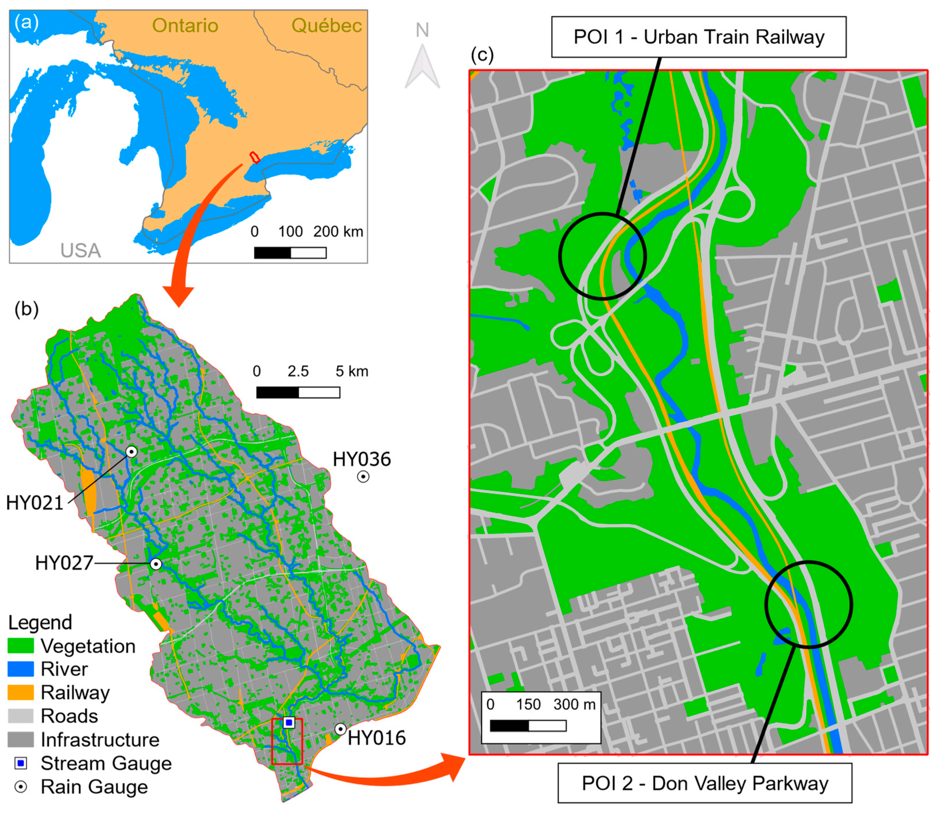
The Don River basin (DRB), located in the Greater Toronto Area, Ontario, Canada, has a total drainage area of nearly 350 km2, approximately 300 km2 of which is located upstream from the river gauge HY019. The baseflow of the Don River recorded by HY019 is approximately 4.5 m3/s. As represented in Figure 1, its landcover is characterized predominantly by urban infrastructure (80%), with disperse portions of sparse tree clusters, wetlands and crops [26]. The region just downstream the HY019 river gauge is often inundated during flash flood events with reports of stranding cars and urban trains in streets and railroads along the riverbanks of the Don River [27,28]. Two locations were selected as points of interest (POI) for further analysis: POI 1 is a segment of the local urban train railway, while the POI 2 is a section of the Don Valley Parkway.
Precipitation data from four rain gauges (HY016, HY021, HY027, HY036) and river discharge data from the river gauge HY019, both with 15 min resolution and ranging from 2011 to 2019, were used to select high-flow rainfall-runoff events. As this study is focused on pluvial flash floods, only the data of the warm seasons (from May to October) of each year were considered to avoid potential influence of snowfall and snowmelt.
3. Materials and Methods
3.1. Physically Based Model Used as Reference
A calibrated semi-distributed hydrologic model of the entire DRB (Figure 1b) was initially developed and provided by the Toronto and Region Conservation Authority (TRCA). The model is based on the Storm Water Management Model (SWMM) [29] and was implemented with the PCSWMM software [30]. The basin is discretized into 462 sub-catchments, each of them set to receive the same precipitation timeseries observed by its nearest precipitation gauge as if it was spatially uniform within the sub-catchment. Water flow is routed through 2703 SWMM conduits (river segments) that reproduce the major rivers and pathways by solving the complete one-dimensional Saint-Venant equation, thus considering the momentum component but without the explicit modeling of surface inundation spread.
The original DRB model was modified to include a hydraulic surface flow component (hereafter referred to as “hydraulic component”) of the aforementioned flood-prone area (Figure 1c). The Digital Elevation Model (DEM) used was obtained from the aggregation of LiDAR products originally provided publicly by the governmental agency Natural Resources Canada at 1 m resolution. The spatial aggregation into 2 m was performed to reduce the negative impact that relatively small surface artefacts, such as sudden spikes or depressions generated by signal noise, may cause to the final simulation results as they can be wrongly interpreted as barriers to the surface water flow [31,32].
In PCSWMM, surface flow is simulated through a dense network of regular SWMM components. A mesh of junctions is established from the underlying DEM, each junction being connected to up to 6 neighbors by 1-segment conduits. Each junction reports the water depth of a location, thus acting (and hereafter referred) as “surface flow cells”. The conduits are modeled as open rectangular cross-sections and perform bi-directional 1D flow routing between two neighboring surface flow cells. Such a configuration allows the simulation of both the lateral and longitudinal water flows needed to represent a 2D surface water movement by solving multiple one-dimensional equations—an approach usually referred to as “quasi-2D”. The flow under crossing bridges is represented by concrete conduits with closed rectangular cross-sections. Manning’s roughness coefficient of the river channel and surrounding vegetated areas were set as 0.01 and 0.05 following the values suggested by Ricketts et al. [33], for open-channel flow over concrete and over light brush on banks, respectively. To represent the flow resistance offered by piers, Manning’s roughness in the channel segments under passing bridges was set to 0.035. Buildings were represented as barriers for the water in the form of regions in the 2D space without surface flow cells.
The hydraulic component of the coupled model is composed by a total of 101,577 cells, 6394 of which are within the river boundaries, 40,482 are floodable cells (i.e., land cells that were inundated in at least one simulation), and the remaining cells are land cells that were not inundated in any simulation.
3.2. Self-Organizing Map (SOM)
SOMs, also known as Kohonen maps after its proposer [34], are among one of the most traditional unsupervised clustering methods in machine learning. An SOM is a specific structure of feed forward artificial neural networks in which the output nodes, representing the clusters, are organized in a 2D topological map. As a clustering technique, each output node of the network refers to a cluster identified for the dataset and has the same number of features as the number of input features. The output nodes in the topological map (hereafter referred simply as “topological nodes”, or TNs) are tuned to be similar to their topological neighbors and, conversely, dissimilar to topologically distant nodes. The process of training starts with a network with randomly defined weights. The records in the training set are successively clustered by the network, i.e., the TN most similar to the clustered record, also called winner node, is identified using a distance function. The winner node then has its weights updated to become more similar to the clustered record through the reduction of the distance value between them by a learning rate α. The other TNs are updated with learning rates that gradually reduce as their topological distance to the winner node increases. Such a gradual reduction is governed by a neighborhood function with parameters defined by the user.
One of its most highlighted features is the capability to successfully cluster [35,36] and provide visual insights [37,38] on high dimensional datasets, which are assets for problems related to flood IMs due to the extensive number of water depth values predicted, one for each inundation cell in the domain. Other applications in water resources include but are not limited to the regionalization of groundwater types [38] and of hydrologic homogeneous watersheds [39], the simulation of daily precipitation [40], and the support of decisions for the operation of reservoirs [41]. The reader is referred to [42] for a further discussion on the use of SOMs in water resources.
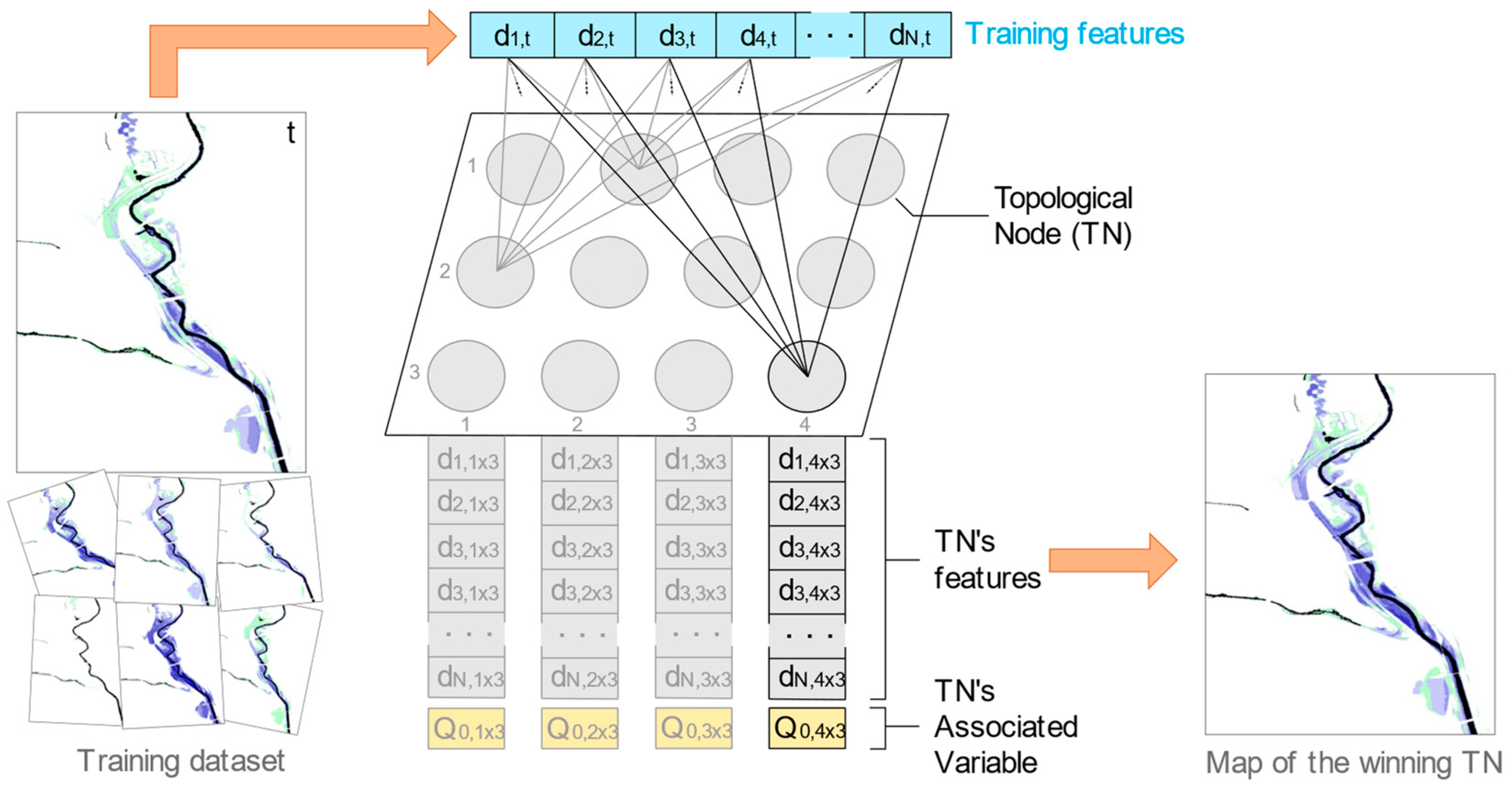
The number of TNs of an SOM is defined by the designer during the model implementation step. As a clustering technique, the higher the number of TNs (clusters), the higher is the expected sharpness of the results and the lower is the degree of generalization of the patterns detected. In this work, SOMs with 12 TNs organized in a 3 × 4 conventional rectangular shape were trained using the water depth values of the 40,482 floodable cells as input features so that each output node can be interpreted as a complete representative IM itself (Figure 2). The total number of 12 TNs was determined heuristically based on the rule-of-thumb suggested by Kohonen [43] of an average of 50 training records per node. Considering the high number of features involved, the total number of training records per node was increased to 100 for a more consistent detection of patterns in the data. The networks were constructed and trained with the MiniSOM library for Python [44] using Gaussian neighborhood and Euclidian distance functions.
To ensure that all records in the train/validation dataset are used for training the data-driven models, 9 SOMs were tuned following the k-fold cross-validation approach, i.e., the records in the train/validation dataset were split into 9 subgroups, then each SOM was trained using 8 of such groups (fold in) and validated against the remaining subgroup (fold out). Hereafter, indicates the SOM validated against the fold-out group . The choice of splitting the records into 9 subgroups was done so that the conventional proportion of 90% training and 10% validation records was achieved (the effective dataset has 17 rainfall events, as discussed in Section 4.1). The training and validation steps are performed concurrently so that, after every fold-in record is presented to the SOM in learning mode, all records in the fold-out group are clustered in prediction mode and the sum of their distances to their respective winner nodes is calculated as . The fold-in records have their order shuffled and the process is repeated so that is calculated. The iteration continues indefinitely while gains in similarity with the validation dataset are observed, i.e., > . Such approach is usually referred as “early stopping criteria” and tends to improve the generalization power of data-driven models [45].
3.3. Recurrent Network
3.3.1. Phase Space Composition
The objective of the recurrent models in this work is to predict the best topological node (and, consequently, the best IM cluster representative) in a specific time in the future given the limited number of hydrological features available in the present. For such, the available dataset needs to be organized in a tabular format so that all the predictive features (inputs) and the respective topological node expected to be predicted (output) are in the same tuple.
Three types of hydrological data were chosen to compose the input set: precipitation (P), discharge (Q) and average inundation depth (AID). P is given as the accumulated average areal precipitation in the sub-catchments of the hydrological model. Initially, at 15 min resolution, P is reconstructed so that is the accumulated precipitation in the interval [t − 2 h, t). Q is the discharge value estimated by the hydrological model in the Don River at the input of the hydraulic domain. Originally at 15 min resolution, Q is reconstructed so that is the mean of the discharge values within the interval [t − 30 min, t). The instantaneous of each calculated by the hydraulic model for time t is given simply by:
in which is the water depth in the floodable cell at time and is the total number of floodable cells in the model.
Each of the train/validation dataset assigned to a record in the fold was clustered by (Section 3.2), thus being associated to a winning topological node of (). Then, 17 phase spaces were constructed, one for each lead time ∈ [0, 15, 30, …, 240] (values in minutes), so that a record for the time in the phase space for is composed by the tuple: , , , , , . The first four elements compose the predictor feature set while the last is the predictand. The data organization is illustrated in Figure 3.
3.3.2. Nonlinear Autoregressive Neural Network with Exogenous Inputs (NARX)
A NARX is a simple recurrent model structured as a conventional feed forward neural network. Its autoregressive component is due the fact that part of the input features depends on the output values predicted by the same model for an antecedent time step. Additional (exogenous) explanatory variables are included in the input set to provide more information to the model. NARX models can be generically described as a mathematical function given by:
in which is the value predicted for time , is the lead time of the forecast (always positive), is an exogenous variable at time , and are the number of previous time steps considered (memory) of the variables and , respectively, and is the estimation error at time that is minimized during the training step. It is worth noting that: (1) multiple exogenous variables can be part of the input feature set, and (2) that the recurrent values may be derived from the previous output values, i.e., an input feature can be, for example, instead of the direct output .
In the original work of Chang et al. [23], a NARX model is trained and used to estimate future AID values using the most recent three-hour accumulated precipitation records observed in three sub-catchments in addition to the last AID value estimated. Such configuration is set up four times, one for each of the four lead times forecasted.
As described in Section 3.3.1, the configuration adopted in our work uses , , , to estimate the probability for each TN to be the winner () for such inputs. From such a set of probabilities and the associated IMs of each TN, the respective is retrieved through interpolation or extrapolation (Section 3.5), from which the required for the prediction of the following step is estimated. Similar to the SOMs configuration, 9 sets of NARX models were tuned according to the training/validation dataset groups. Each set f is composed by 17 models, one for each phase space constructed towards a lead time .
All models trained were composed by a three-layer feed forward neural network structure (one input, one hidden and one output layers). Rectified Linear Unit (ReLu) [46] was set as the activation function of the input and hidden layers, while Softmax [47] was used as the activation function of the output layer. The size of the output layer was 12, each output node of the matching a topological node of the respective model. In such a configuration, the 12 values predicted by the Softmax function represent the probability of each SOM topological map to be the correct one for a given input. The networks were trained to optimize the Categorical Cross-Entropy loss function, which is usually considered as a standard loss function for multi-class classification tasks. The criterion adopted for early stopping is the increase of loss in the validation dataset between each epoch.
The number of nodes in the hidden layer was not defined a priori. For each combination of and , 8 neural networks were trained, each with a different number of hidden nodes ranging from 5 to 12. The configuration that presented the best (lowest) validation loss was taken as the and the others were discarded.
3.4. Update SOMs with Associated Variables
After training, the SOMs were updated to have values of linked to their topological nodes as additional variables. is the instantaneous discharge value at time , thus each has a respective . The of a topological node is calculated as the mean of the values associated with all clustered as part of .
3.5. Hybrid Model Structure
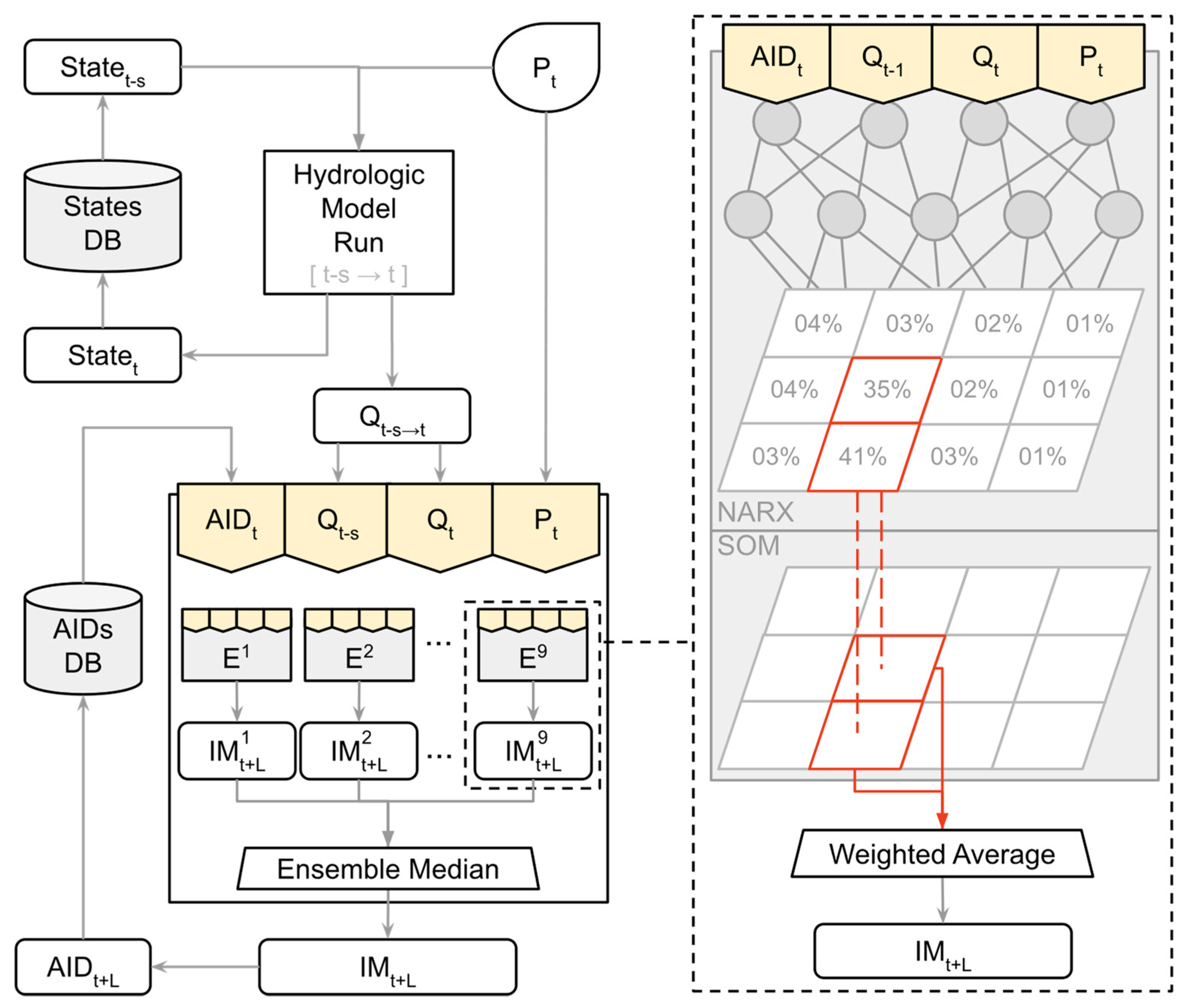
Each pair of and is considered a hybrid model that receives the 4-variables input for the NARX models and outputs an IM derived from the SOM topological nodes for the lead time . The 9 hybrid models set up for a lead time are used simultaneously to produce ensemble forecasts. Such a strategy is often named multiple predicting cross-validation and the merged product of the ensemble members tends to be more consistent than the prediction performed by a single model through conventional approaches [48]. A schematic representation of the reproduced forecasting system applying the dual NARX-SOM is presented in Figure 4. Due to the lack of descriptive data of observed inundation flood maps, the discharge produced by the hydrologic model was assumed to be a realistic response from the catchment to a forcing precipitation data. In an operational environment, however, the simulated discharge data can be replaced by observations if real-time stream gauges are timely available, or discharge forecasts produced by the hydrologic model.
The 9 individual inundation maps forecasted for a certain lead time are aggregated into a single, deterministic map through the Conditional Median/Mean Function (CMMF). CMMF simply defines the water depth value of the floodable cell n as either the mean or the median value of the water depths predicted by all ensemble members to the same node n, represented as the multivariate , by:
CMMF is used as an alternative to the direct application of the elementwise mean value to ensure that nodes more likely to be dry (i.e., that had its water depth predicted to be zero by most of the ensemble members) are not set as wet due to the results of a minority of the members. The aggregation of multiple ensemble forecasts has the potential to smooth out oscillations detected in independent realization that are potentially caused by overfitting [22].
The topologic node with higher value of AID of each SOM model trained is labeled as the most extreme inundation scenario learned. Such identification is used to determine whether the predicted inundation map should be estimated by the interpolation or extrapolation of the learned patterns. If the winner topologic node is the most extreme one and its estimated probability is above 50%, then it is assumed that the input will produce an inundation condition potentially not covered in the train/validation dataset and thus an extrapolation from the most extreme scenario shall be performed. The extrapolation is performed by the multiplication of the water depths of the most extreme inundation scenario learned by a factor α, given by:
in which is the most recent input discharge in the as predictive feature set, is the most recent input discharge associated with the winner topologic node, is a decay factor, is the lead time of the forecast, and is the temporal resolution. The inclusion of a decay factor aims to simulate an expected reduction of future input discharge after the observation of extreme conditions (the higher the value of , the more intense is the decay). The value used influences the performance of the maps generated outside of the training data space and reflects the expectations of the implementers concerning the intensity of possible future extreme rainfall events. In this work, a decay factor of 0.03 was utilized after experiments performed in the train/validation dataset.
For all other scenarios, the IMs of the two topologic nodes with highest estimated probabilities are interpolated by the weighted averaging, so that the interpolated IM estimated for a lead time , , is calculated as:
in which and are the water depth values of the floodable cells of the topologic node with the first and second highest estimated probabilities and , respectively.
3.6. Train/Validation and Test Datasets
A total of 87 significant rainfall-runoff events were initially extracted from the available gauge data (described in Section 2). In this work, a rainfall-runoff event is characterized as “significant” if a precipitation record is followed by an increase in the discharge recorded at the HY019 gauge of 2 times the magnitude of the regular baseflow or more. All intense rainfall events were equally set to have total duration of 24 h, starting 12 h before and ending 12 h after its peak precipitation record. As the observed precipitation data were kept unmodified, this set of rainfall events are named RE-O (Rainfall Events—Observations) hereafter.
A set of 87 synthetic rainfall events were generated out of the RE-O dataset through the shuffling of the precipitation timeseries observations within the same event (e.g., as if the gauge HY036 had recorded what was recorded by the HY027 gauge, and as if HY027 had recorded what was recorded by HY021, and so on until all timeseries were set to a gauge different from its original gauge). Such a spatial disturbance of past observations through shuffling the location of observations is assumed to be a realistic “what-if” scenario. This set of records is named RE-SS (Rainfall Events—Synthetic by Shuffling) hereafter.
The 10 RE-O events with highest observed peak flows were selected to compose the RE-OH (Rainfall Event—Observed Highest) set. An additional augmentation was performed on the RE-OH events by a simple increase of 10% of all values of the timeseries. The resulting synthetic events represent scenarios of more intense, less recurrent events that could be observed but were not captured in the considered data period. This set is named RE-SE (Rainfall Events—Synthetic by Extrapolation) hereafter. A summary of the intermediate datasets is presented in Table 1.
All records of RE-O, RE-OH, RE-SS and RE-SE were used as the precipitation forcing for the hydrologic-hydraulic model starting from a baseflow steady condition. The simulated IMs and river discharge at HY019 were recorded with a temporal resolution of 15 min to match the temporal resolution of the precipitation dataset.
The 194 simulated events were subsampled to reduce redundancies. Then, two disjoint subsets of the subsampled set were built through manual selection of records to compose the train/validation and the test datasets, respectively. This selection was performed to reduce the imbalance of the original datasets in which higher recurrence events, usually of lower intensity, are predominant. The events in the train/validation dataset were randomly split into 9 groups (or “folds”) for the application of k-fold cross-validation technique in the tunning of both the SOM and the NARX models.
3.7. Evaluation Metrics
The performance of the NARX models on predicting the correct SOM topological node was performed through a binary approach using accuracy as the metric, i.e., the topological node deterministically predicted by the NARX model was compared to the topological node obtained by direct SOM classification of the respective inundation map. The total number of correct predictions () and the total number of predictions evaluated () were used to estimate the overall accuracy as:
Accuracy values range from 0 (no correct predictions detected) to 1 (perfect predictive power).
Three metrics were used to evaluate the performance of the hybrid model so that average error, variance replicability and bias of the studied models can be assessed.
The coefficient of determination (R2) calculates the goodness of the fit of an estimation to a reference dataset in terms of variance replicability. It has values ranging from 0 (worse possible) to 1 (perfect) and is calculated as the square of the Pearson correlation coefficient , i.e.,
in which is the total number of records, is the mean value of the reference dataset, and and are the i-th reference and estimated values, respectively.
The root mean square error (RMSE) estimates the average error magnitude in the estimations from a model given in the same unit as the evaluated variable (meters in this work), with 0 meaning perfect match and no upstream value constraint. RMSE is given by:
Bias is calculated by the relative percent difference of the predictions to the observations, being calculated by:
A positive bias value represents overestimation while a negative value indicates underestimation, both bounded by 2 and −2, respectively. The closer the bias value is to 0, the less biased is considered the model. This approach to calculate bias was selected due to its tolerance to zero values, be it in the reference or in estimation.
Contingency tables synthetize the performance of a model in predicting the occurrence of a certain type of event through the number of true positives (or “hits”, H), false negatives (or “misses”, M), false positives (or “false alarms”, F) and true negatives (or “correct no-alarm”, N). In the context of contingency analysis of this work, the occurrence of an “event” is determined by the exceedance of the water depth in a floodable cell over a given threshold during any moment of a time interval. In this work, water depths of 10, 25, 50, 100 cm were considered as thresholds representing the respective conditions of minor, moderate, high and major threat for the traffic of cars and urban trains.
Contingency metrics considered in this work are the probability of detection (POD), the Success Ratio (SR) and the Critical Success Index (CSI) at the 2 POIS for the prediction of multiple maximum water depths. POD is a metric of sensibility and has values ranging from 0 (completely insensitive, i.e., unable to predict any tested event) to 1 (completely sensitive, i.e., able to predict all tested events) and is given by:
while SR is a metric of reliability also with values between 0 (completely unreliable, i.e., no forecasted events were observed) and 1 (completely reliable, i.e., all forecasted events were observed), and is calculated by:
There is a usual trade-off between the POD and the SR metrics: while models characterized by overestimated predictions tend to have high POD and low SR scores, models with underestimated prediction forecasts tend to present the opposite POD/SR relationship. As both sensibility and reliability are important features for predicting floods, such duality may turn the task of evaluating the overall performance of models to be subjective. The CSI metric can be seen taken as an objective metric that balances both the abovementioned characteristics and is calculated as:
with values ranging from 0 (worse possible with no correct prediction) to 1 (best possible with no miss predictions). By not taking into consideration the component N, CSI values tend to be numerically lower than accuracy values in circumstances in which non-event records significantly outnumber event records, as for the prediction of low recurrence flood events. Given such consideration, we assume in this work that a model must have a minimum CSI of 0.8 to be considered useful for flood forecasting from the perspective of decision makers. This can be considered a conservative threshold after the minimum accuracy of the same value as reported by [49] for a catchment also managed by TRCA.
4. Results and Discussion
4.1. Selected Rainfall-Runoff Events
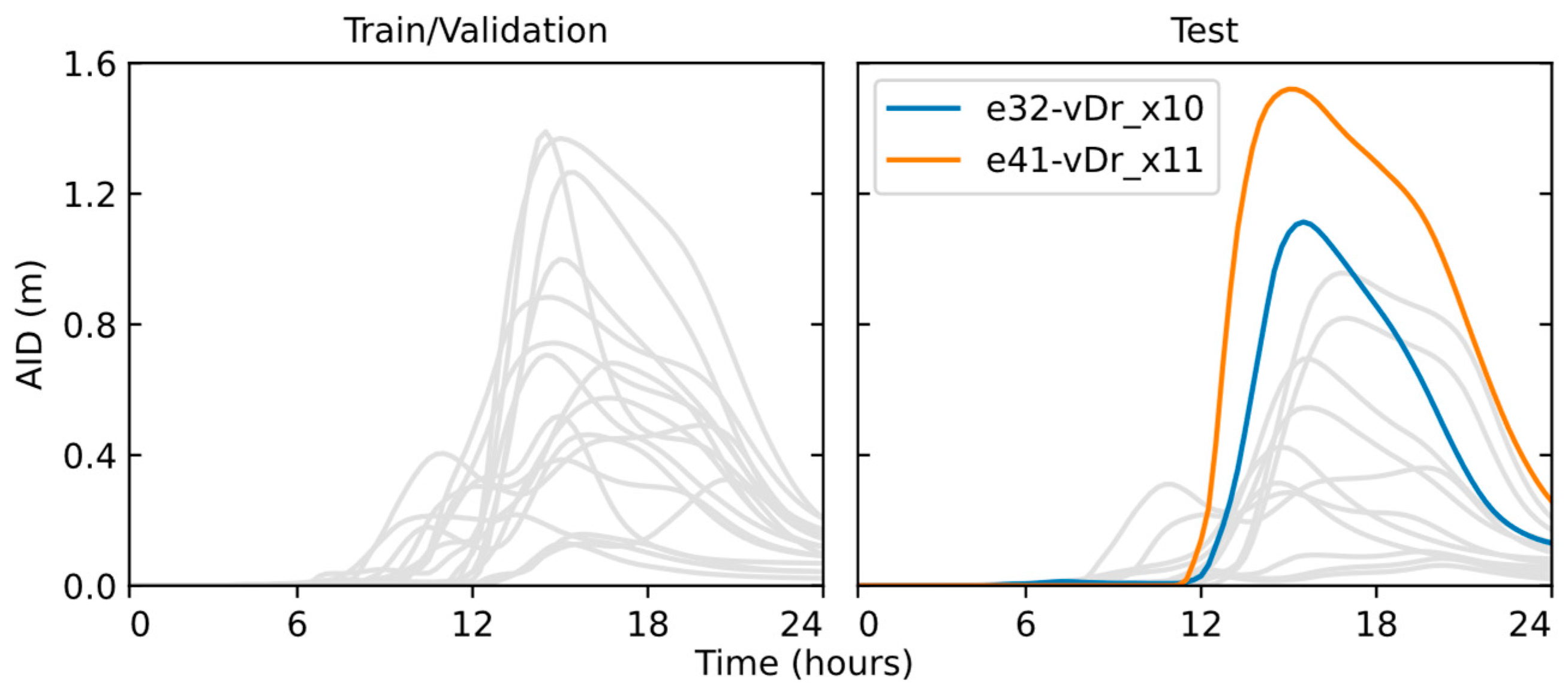
Table 2 presents the overall characteristics of the 24 h events selected for the tuning and evaluation of the data-driven models. To reduce overbias of the model towards highly recurrent scenarios, several rainfall events with low maximum AID (lower than 0.15 m) were discarded. A total of 30 events were effectively used out of the 194 initial simulations performed, 17 of which composed the train/validation dataset while the remaining 13 composed the test dataset. The most extreme event, identified as e41-vDr_x11, was included in the test dataset so that the performance of the model for extrapolating results could be assessed. Figure 5 shows the AID timeseries of all selected events and illustrates the data distribution of each dataset, with the timeseries of the two events used as study case scenarios (Section 4.4.2) highlighted.
4.2. Assessment of the SOM Models Trained
As discussed in Section 3.2, nine SOM networks were trained using the k-fold cross validation approach, each of which have 3 × 4 topological dimension and output node weights representing the water depth at individual cells of the 2D predicted inundation map. Figure 6 presents the topological nodes of one of the nine SOMs trained to illustrate their overall organization. As expected, it can be observed a gradual increase of the flood extension and overall water depth from the map with virtually no flooding (node 1 × 3) to the map related to the most extreme conditions (node 4 × 1). The consistency of the inundation maps obtained demonstrate that SOM is able to properly cluster high-resolution grids (i.e., high number of features) with a relatively limited number of inundation maps used as samples for training (1320 IMs) and validating (176 IMs). Linear discontinuities through the inundated area and river path are due to the existence of crossing bridges, which are modeled in SWMM as closed conduits to represent their underneath water pathways instead of nodes that are interpreted as floodable cells.
It is also interesting to note that the four maps in the top left corner of Figure 5 may be taken as scenarios of concern for the POI 2 while all scenarios in columns 3 and 4 may result in the need of actions for POI 1. In an operational setting, such a configuration could be used as additional information to improve the perception of imminent risk through the interpretation that the topologically closer a predicted winner node is to these “clusters of clusters”, the higher should be the awareness level of the forecasters.
4.3. Assessment of the NARX Models Trained
As discussed in Section 3.3, eight NARX models were trained for each of the 17 lead times predicted for each of the nine folding groups, resulting in a total of 1224 models trained, 153 of which were selected as the ones with the best performance. There was not a predominant set of hyperparameter values in the selected models, which corroborates with the general concept that each independent problem may have different optimal network structures.
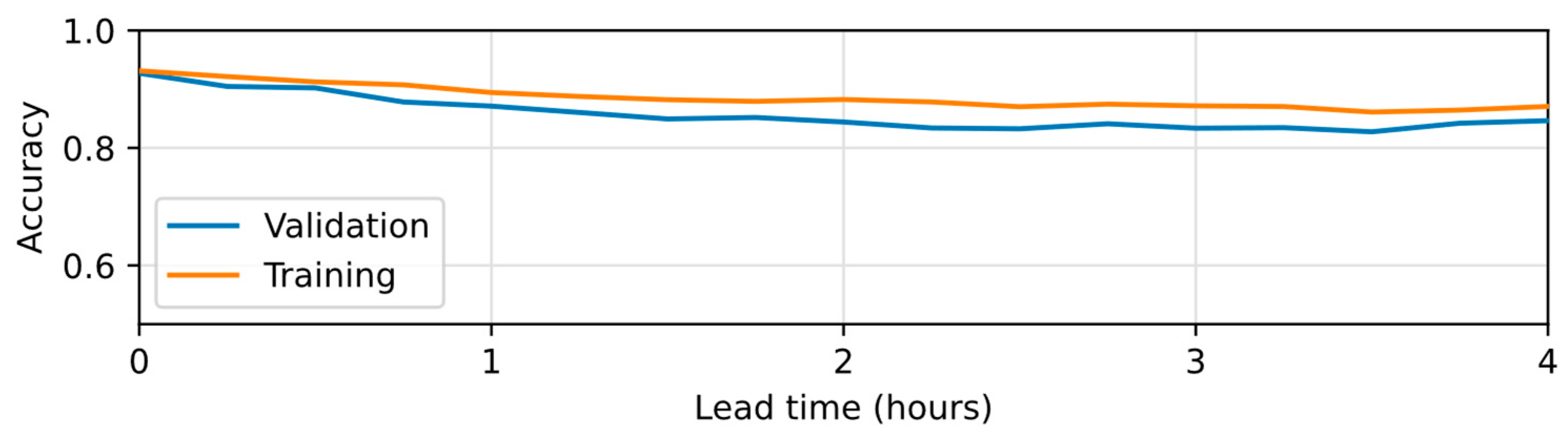
The accuracy of the selected NARX models on predicting the correct topological node of its related SOM out of the hydrological features is presented in Figure 7. As expected, the predictive performance on the training dataset is superior to the performance on the validation dataset, but the relatively small difference between their accuracy values indicates an acceptable degree of generalization. As also expected, the overall performance of the classifier decreases as the lead time of the prediction increases from the lowest lead time up to a lead time of 2 h, after which the performance only oscillates around a constant value. As the response time of the catchment is also in the order of 2 h, the discontinuity can be explained by the influence of precipitation and discharge in the earlier lead times, while for longer lead times the performance is influenced almost completely by the recurrent variable of AID. The performance obtained was superior to 80% for all lead times; however, such a result must be observed with discretion as the AID values used as part of the predictive feature sets were calculated from the IMs simulated by the physically based model instead of being derived from estimations of the outputs from the surrogate model for previous time steps. Such a configuration represents an ideal scenario in which the surrogate model reproduces with perfection the physically based model.
It is worth noting that a misclassification may still be considered a useful classification if the predicted TN neighbored the correct TN, which would result in a low overall error due to their similarities. The global error of the combined model is explored in Section 4.4.
4.4. Assessment of the Hybrid Model
4.4.1. Global Performance
After both SOM and NARX models were trained using the train/validation dataset, the effective performance of the hybrid model was assessed using the testing dataset in an operational setup, i.e., with the value of the recurrent feature AID being obtained from the inundation map latest predicted in previous steps.
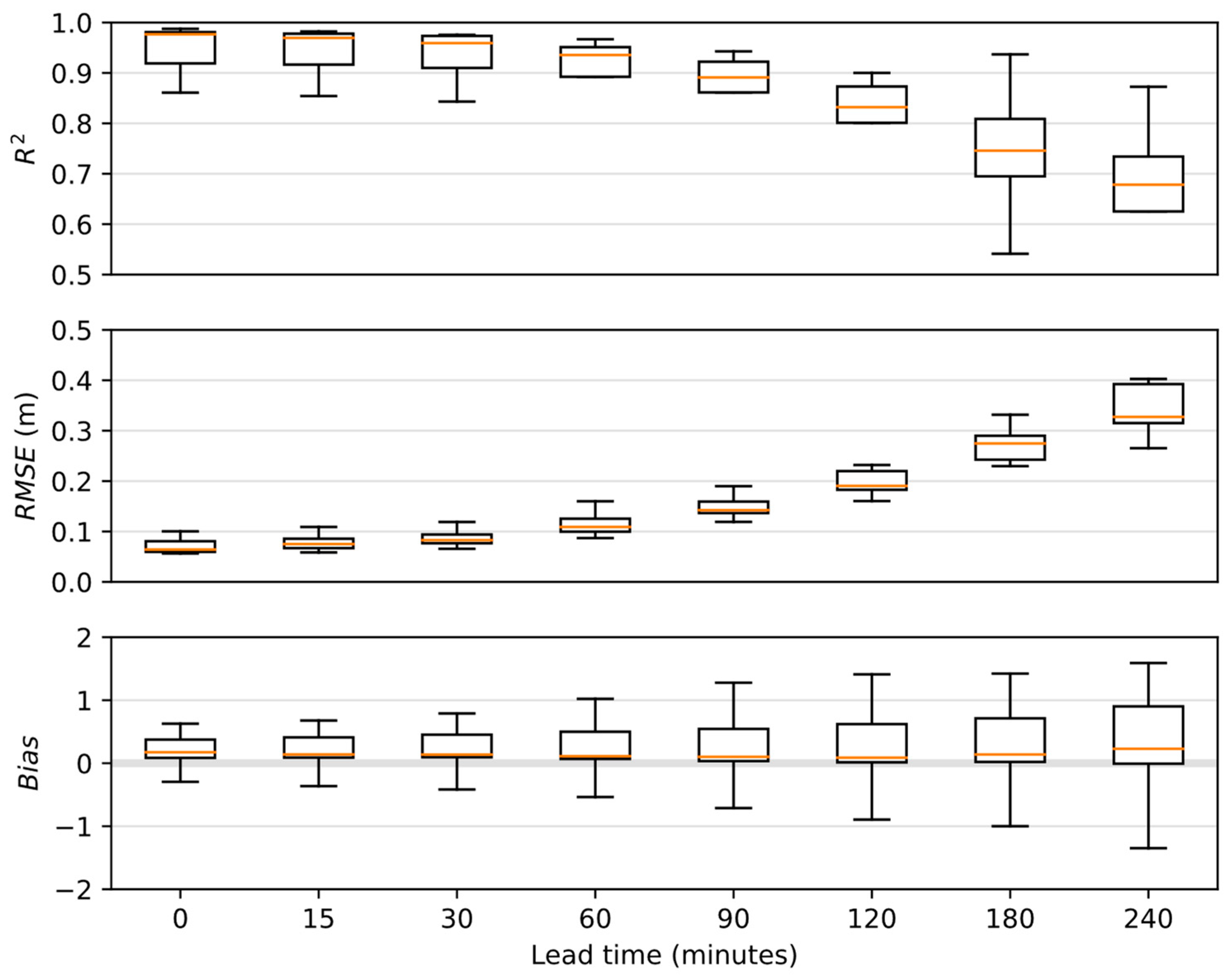
Figure 8 shows the performance of the forecasts in terms of R2, RMSE and bias for the different lead times considered. The higher degradation in performance with respect to the lead time when compared to the NARX analysis is due the cumulative error carried with the sequential estimation of AID values. Results were considered acceptable for the lead time of up to 2 h (120 min) in terms of both R2 (above 0.8) and RMSE (bellow 0.25 m). All lead times presented low overall bias; however, the significant spread for lead times longer than 1.5 h (90 min) indicates a high level of uncertainty that can be considered a constraint for decision makers. The slight trend towards overestimation can be induced by the loss function used during the training of the NARX models, which prioritizes the correct classification of less recurrent (in our case, more intense) events over more common (and thus less intense) events.
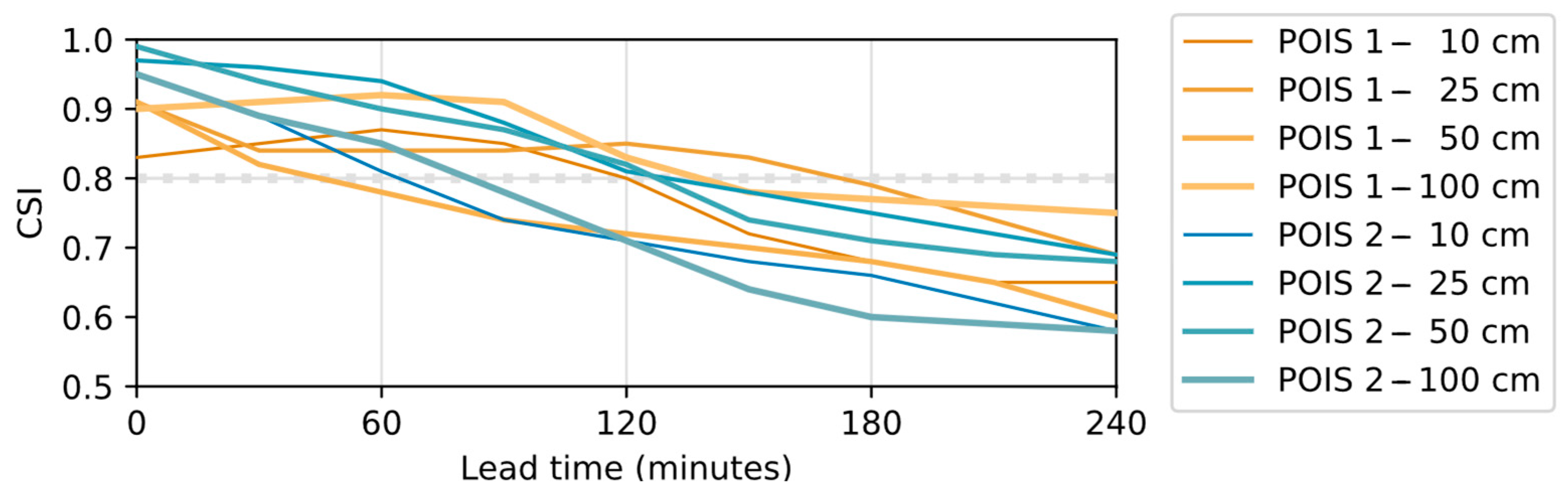
The forecasts were able to satisfactorily predict the occurrence of flood conditions at different depths on both POIs (Table 3 and Table 4). The aforementioned tendency to overestimate the forecast is reflected in highs level of sensitivity (POD), allowing the early detection of more than 90% of the upcoming events in most of the cases and increasing with longer lead times. However, as the sensitivity increases with longer lead times, the number of false alarms issued also increases, which disproportionately decreases the reliability (SR) of the predictions and consequently reduces the overall skill of the model (CSI). CSI is higher than 0.8 for maximum lead times ranging from 30 min (POI 1 for a threshold of 50 cm) up to 150 min (POI 1 for threshold of 25 cm), which indicates that the proposed system can be useful to forecasters. The overall better performance to detect events in the POIS 2 for early lead times when compared to the POIS 1 (Figure 9) can be explained by the different location and surrounding areas of each point. POIS 2 is located close to the margin of stream and is not subject to pounded water, which leads to its water depth to be highly correlated to the instantaneous river water depth. Conversely, the POIS 1 has its behavior more correlated to longstanding flow conditions due to its longer distance from the stream margin and its surrounding micro-relief to be subject to pounded water, which results in better prediction performances at longer lead times.
4.4.2. Performance on Selected Events
The two most extreme events of the testing dataset (highlighted in Figure 5) were selected as study cases. The first event (e32-r-x10) refers to the storm event observed during the night of 29 May 2013, which caused a temporary interruption of the urban train operations and the partial submersion of cars due to inundations in the POIs [50]. Such a rainfall event has a magnitude below the most extreme event in the train/validation dataset, thus it is expected to be reproduced by the hybrid model from the interpolation of its “known” events. The second event (e41-r-x11) simulates the storm event that was observed less than two months after the first one, on 9 July 2013, when several passengers had to be rescued from an urban train strained in the POI 1, and the road traffic was interrupted in the POI 2 due to river overbank conditions [51]. It has a magnitude above the most extreme scenario of the train/validation dataset, thus serves to assess the capabilities of the hybrid model to perform predictions through extrapolation of learned patterns.
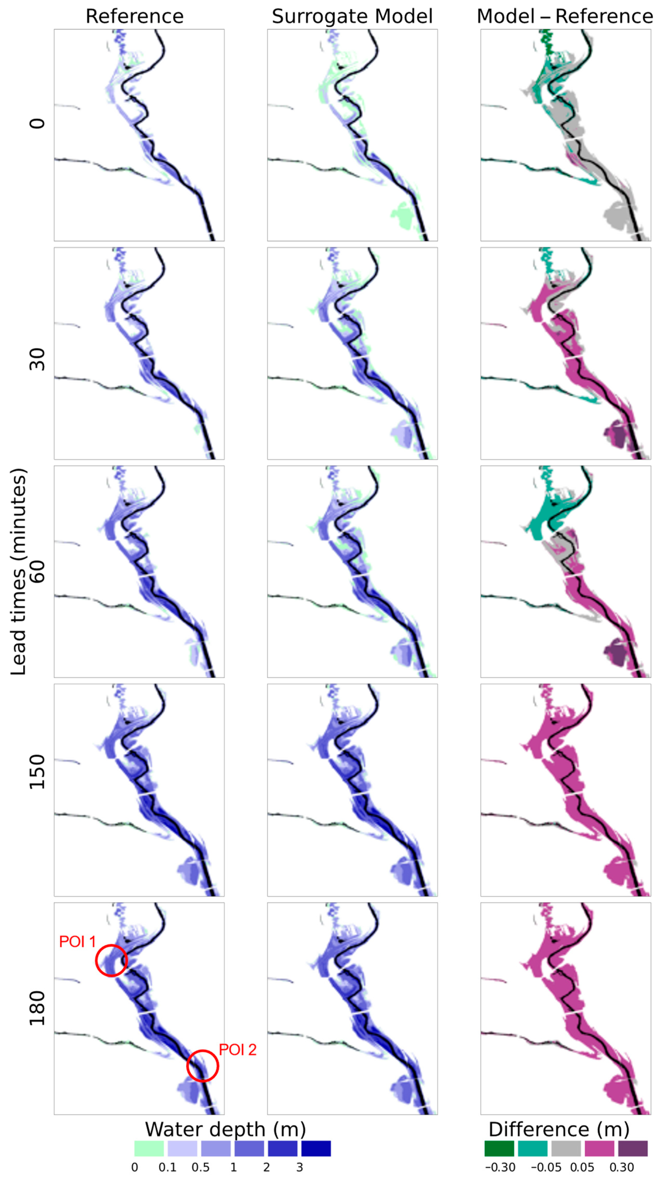
A comparison between IMs produced by the physically based model for the event e32-r-x10 and the respective predictions generated by the surrogate model at a fixed issue time is shown in Figure 10. It is possible to observe that there is little deviation from the simulation in the estimation for the present-moment condition, and as that the error due to overestimation tends to increase as lead time increases. Despite such errors, the overall development of the inundation is properly reproduced, and decision makers responsible for closing (or not) the road at the POI 2 would be properly informed that a minor to moderate inundation scenario would occur in the upcoming 30 min, while a moderate to major condition would be attained within 60 min. A similar result can be observed at the POI 1 in spite of its early underestimation of the water depth.
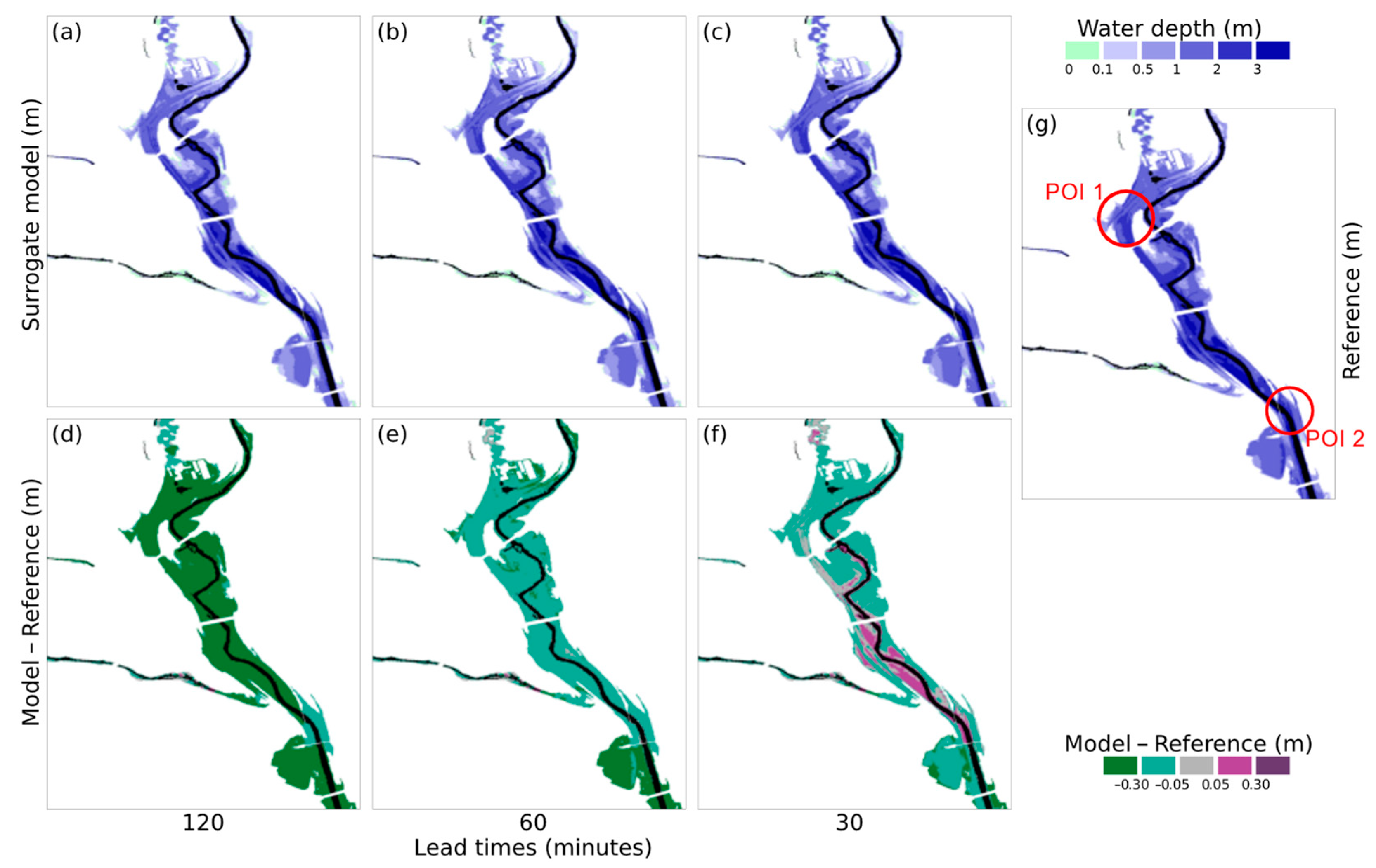
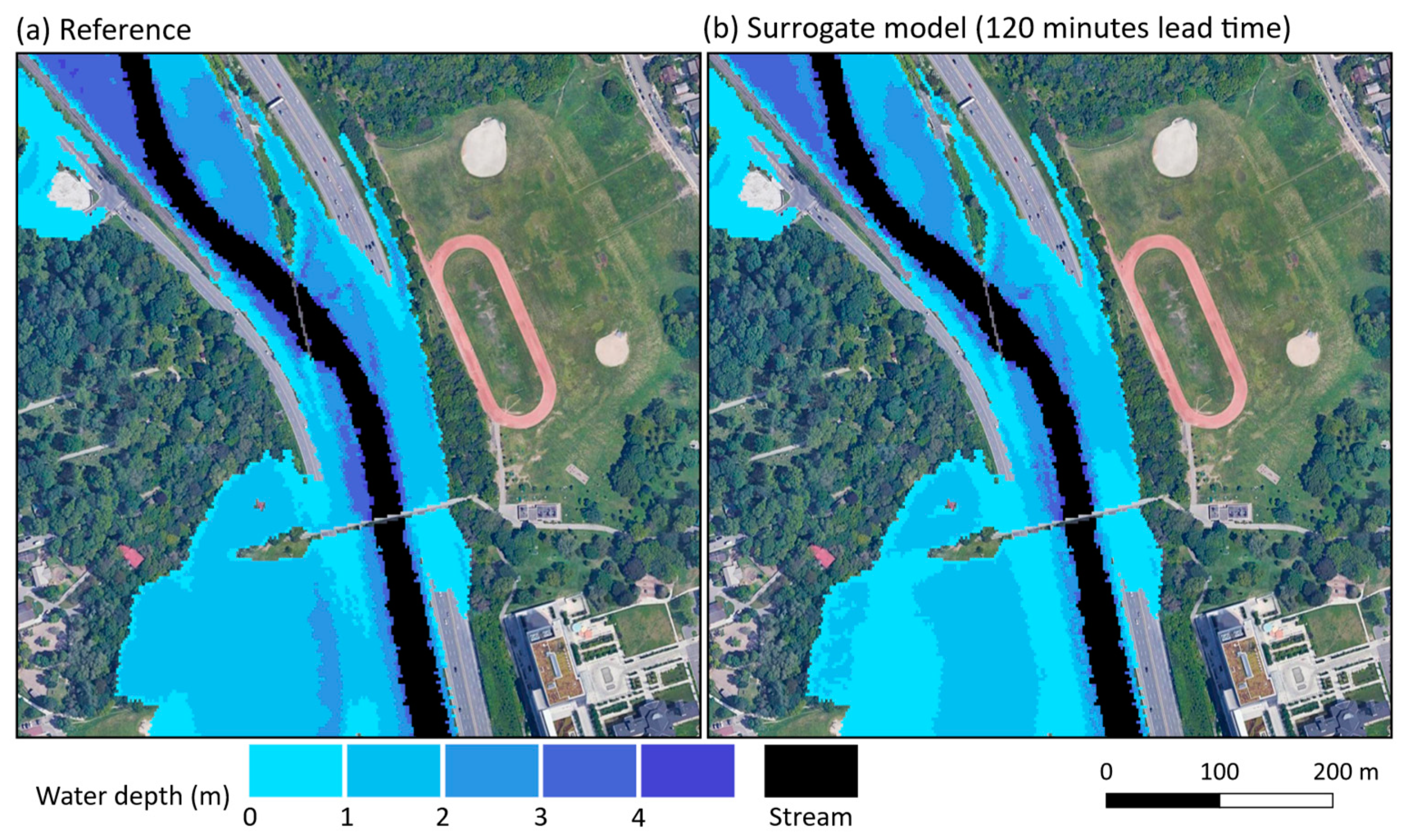
The overall maps issued at different lead times for the peak inundation condition of the event e41-r-x11 and their comparison with the maps produced by the physically based model are shown in Figure 11. As it can be observed, IMs with high overall similarity are forecasted up to 2 h ahead of the most extreme condition despite some significant underestimation. Figure 12 shows a local view of the POI 2 with the maps produced directly by PCSWMM and by the surrogate model, illustrating how the overall inundation pattern is properly reproduced, and how the forecasters would be notified that the roads along the riverbank would have points in which water height ranges between 1 to 2 m. As the lead time decreases (i.e., as the issue time approximates the peak inundation time) and more precipitation and discharge data become available, the overall underestimation of the water depth also gradually significantly decreases, thus illustrating the effects of recent data on “correcting” previously issued predictions (Figure 11b,c,e,f).
4.5. Runtime Comparison
A computer with the following specifications was used to compare the runtime of both the hydrologic-hydraulic model and its surrogate counterpart: CPU Intel I9 with 3.6 GHz, eight cores and 16 logical processors; 64 GB memory RAM. The execution of the physically based hydraulic model for a simulation time of 4 h took 4.5 h to complete, confirming its unsuitability for real-time operational purposes. On the other hand, the generation of the inundation maps for all lead times up to 4 h ahead of the same event took the order of 11 to 15 min, which can be considered compatible to operational forecasting setups. It is worth mentioning that the hybrid models were executed without parallel processing and thus have the potential to have their execution time reduced if such techniques are applied.
4.6. Contraints and Limitations of the Methodology
As a surrogate model, the operational adoption of the proposed methodology depends on a pre-existing hydrological/hydraulic model to be available and properly configured. The implementation of such models, however, depends on the availability of detailed information of the study area, such as high-resolution DEMs and drainage systems, which may not be guaranteed for specific locations.
To maintain a proper replication of the physically based model used as reference, the surrogate model needs to be retrained every time the physically based model is modified. Such updates may be performed with certain recurrence to include, for example, significant structural changes in the covered domain (such as changes in the land use) or recalibrations to consider changes in the rainfall regimes induced by climate change.
5. Conclusions and Future Works
This work presents evidence that hybrid NARX-SOM models can be effective in predicting inundation maps for flash floods caused by river overflow of catchments with short response time. The promising results were obtained using a restrict number of training events, which can be considered an appealing feature as eventual retraining of the hybrid models would require limited re-simulations of the hydraulic model. Forecast products were considered valuable for decision makers for lead times ranging from 30 min to 2.5 h, which can be considered acceptable for the purposes of closing streets to traffic and stopping the operation of trains. To increase the lead time, the use of precipitation forecasts should be considered and are the potential subject of future studies. In the current study, multiple predictors were trained independently using the cross-fold approach and a simple aggregation of their predictions was used as deterministic forecasts. The production of probabilistic flood inundation maps [13] is of continued interest, and future works will explore the potentials of the dual NARX-SOM approach to produce inundation maps accompanied with consistent uncertainties. In addition, the presented results are limited to a single study scope and further experiments are expected to be developed to further assess its applicability to other scenarios.
Author Contributions
Conceptualization, implementation, and writing—original draft preparation, A.D.L.Z.; writing—review and editing, supervision, project administration, funding acquisition, P.C.; all authors contributed equally to the discussion over the results and contributed to the final manuscript. All authors have read and agreed to the published version of the manuscript.
Funding
This research was supported by the Natural Science and Engineering Research Council (NSERC) of Canada, grant NSERC Canadian FloodNet (NETGP-451456).
Data Availability Statement
Publicly available datasets were analyzed in this study. This data can be found at: https://data.trca.ca/dataset (accessed on 19 January 2022). The hydrological-hydraulic model used in this work is not publicly available as it is a property of the Toronto and Region Conservation Authority (TRCA).
Acknowledgments
The authors would like to thank the Toronto and Region Conservation Authority (TRCA) for providing the original hydrological model and the data used in this work, and Computational Hydraulics International (CHI) for providing an academic license of PCSWMM software for this study.
Conflicts of Interest
The authors declare no conflict of interest.
Abbreviations
| Acronyms | Meaning |
| AID | Average inundation depth |
| CMMF | Conditional Median/Mean Function |
| CSI | Critical Success Index |
| DEM | Digital Elevation Model |
| DRB | Don River Basin |
| EP | Estimated probability |
| NARX | Nonlinear Autoregressive neural network with exogenous inputs |
| POD | Probability of detection |
| POI | Point of interest |
| RE-O | Rainfall Events—Observations |
| RE-OH | Rainfall Events—Observations (Highest) |
| RE-SS | Rainfall Events—Synthetic by Shuffling |
| RE-SE | Rainfall Events—Synthetic by Extrapolation |
| RMSE | Root mean square error |
| SOM | Self-Organizing Maps |
| SR | Success Ratio |
| SWMM | Storm Water Management Model |
| TN | Topological node |
References
- WMO—World Meteorological Organization. Climate and Water; WMO: Geneva, Switzerland, 2020; Volume 69. [Google Scholar]
- Lehmann, J.; Coumou, D.; Frieler, K. Increased Record-Breaking Precipitation Events under Global Warming. Clim. Chang. 2015, 132, 501–515. [Google Scholar] [CrossRef]
- Zhao, G.; Gao, H.; Cuo, L. Effects of Urbanization and Climate Change on Peak Flows over the San Antonio River Basin, Texas. J. Hydrometeorol. 2016, 17, 2371–2389. [Google Scholar] [CrossRef]
- Sofia, G.; Roder, G.; Dalla Fontana, G.; Tarolli, P. Flood Dynamics in Urbanised Landscapes: 100 Years of Climate and Humans’ Interaction. Sci. Rep. 2017, 7, 40527. [Google Scholar] [CrossRef] [PubMed]
- Modrick, T.M.; Graham, R.; Shamir, E.; Jubach, R.; Spencer, C.R.; Sperfslage, J.A.; Georgakakos, K.P. Operational Flash Flood Warning Systems with Global Applicability. In Bold Visions for Environmental Modeling, Proceedings of the 7th International Congress on Environmental Modelling and Software (iEMSs 2014), San Diego, CA, USA, 15–19 June 2014; Brigham Young University: Provo, UT, USA; pp. 694–701.
- Hapuarachchi, H.A.P.; Wang, Q.J.; Pagano, T.C. A Review of Advances in Flash Flood Forecasting. Hydrol. Process. 2011, 25, 2771–2784. [Google Scholar] [CrossRef]
- Zanchetta, A.D.L.; Coulibaly, P. Recent Advances in Real-Time Pluvial Flash Flood Forecasting. Water 2020, 12, 570. [Google Scholar] [CrossRef] [Green Version]
- Costabile, P.; Costanzo, C.; de Lorenzo, G.; Macchione, F. Is Local Flood Hazard Assessment in Urban Areas Significantly Influenced by the Physical Complexity of the Hydrodynamic Inundation Model? J. Hydrol. 2020, 580, 124231. [Google Scholar] [CrossRef]
- Nobre, A.D.; Cuartas, L.A.; Hodnett, M.; Rennó, C.D.; Rodrigues, G.; Silveira, A.; Waterloo, M.; Saleska, S. Height Above the Nearest Drainage—A Hydrologically Relevant New Terrain Model. J. Hydrol. 2011, 404, 13–29. [Google Scholar] [CrossRef] [Green Version]
- Follum, M.L.; Tavakoly, A.A.; Niemann, J.D.; Snow, A.D. AutoRAPID: A Model for Prompt Streamflow Estimation and Flood Inundation Mapping over Regional to Continental Extents. J. Am. Water Resour. Assoc. 2017, 53, 280–299. [Google Scholar] [CrossRef]
- Samela, C.; Persiano, S.; Bagli, S.; Luzzi, V.; Mazzoli, P.; Humer, G.; Reithofer, A.; Essenfelder, A.; Amadio, M.; Mysiak, J.; et al. Safer_RAIN: A DEM-Based Hierarchical Filling-&-Spilling Algorithm for Pluvial Flood Hazard Assessment and Mapping across Large Urban Areas. Water 2020, 12, 1514. [Google Scholar] [CrossRef]
- Hu, A.; Demir, I. Real-Time Flood Mapping on Client-Side Web Systems Using Hand Model. Hydrology 2021, 8, 65. [Google Scholar] [CrossRef]
- Teng, J.; Jakeman, A.J.; Vaze, J.; Croke, B.F.W.; Dutta, D.; Kim, S. Flood Inundation Modelling: A Review of Methods, Recent Advances and Uncertainty Analysis. Environ. Model. Softw. 2017, 90, 201–216. [Google Scholar] [CrossRef]
- Hocini, N.; Payrastre, O.; Bourgin, F.; Gaume, E.; Davy, P.; Lague, D.; Poinsignon, L.; Pons, F.; Bouguenais, F.; Rennes, G.; et al. Performance of Automated Methods for Flash Flood Inundation Mapping: A Comparison of a Digital Terrain Model (DTM) Filling and Two Hydrodynamic Methods. Hydrol. Earth Syst. Sci. 2021, 25, 2979–2995. [Google Scholar] [CrossRef]
- Jan, A.; Coon, E.T.; Graham, J.D.; Painter, S.L. A Subgrid Approach for Modeling Microtopography Effects on Overland Flow. Water Resour. Res. 2018, 54, 6153–6167. [Google Scholar] [CrossRef]
- Cao, X.; Ni, G.; Qi, Y.; Liu, B. Does Subgrid Routing Information Matter for Urban Flood Forecasting? A Multiscenario Analysis at the Land Parcel Scale. J. Hydrometeorol. 2020, 21, 2083–2099. [Google Scholar] [CrossRef]
- Nkwunonwo, U.C.; Whitworth, M.; Baily, B. Urban Flood Modelling Combining Cellular Automata Framework with Semi-Implicit Finite Difference Numerical Formulation. J. Afr. Earth Sci. 2019, 150, 272–281. [Google Scholar] [CrossRef] [Green Version]
- Dazzi, S.; Vacondio, R.; Dal Palù, A.; Mignosa, P. A Local Time Stepping Algorithm for GPU-Accelerated 2D Shallow Water Models. Adv. Water Resour. 2018, 111, 274–288. [Google Scholar] [CrossRef]
- Ming, X.; Liang, Q.; Xia, X.; Li, D.; Fowler, H.J. Real-Time Flood Forecasting Based on a High-Performance 2-D Hydrodynamic Model and Numerical Weather Predictions. Water Resour. Res. 2020, 56, e2019WR025583. [Google Scholar] [CrossRef]
- Razavi, S.; Tolson, B.A.; Burn, D.H. Review of Surrogate Modeling in Water Resources. Water Resour. Res. 2012, 48, 7401. [Google Scholar] [CrossRef]
- Bermúdez, M.; Cea, L.; Puertas, J. A Rapid Flood Inundation Model for Hazard Mapping Based on Least Squares Support Vector Machine Regression. J. Flood Risk Manag. 2019, 12, e12522. [Google Scholar] [CrossRef] [Green Version]
- Berkhahn, S.; Fuchs, L.; Neuweiler, I. An Ensemble Neural Network Model for Real-Time Prediction of Urban Floods. J. Hydrol. 2019, 575, 743–754. [Google Scholar] [CrossRef]
- Chang, L.-C.; Amin, M.; Yang, S.-N.; Chang, F.-J. Building ANN-Based Regional Multi-Step-Ahead Flood Inundation Forecast Models. Water 2018, 10, 1283. [Google Scholar] [CrossRef] [Green Version]
- Kim, H.I.; Keum, H.J.; Han, K.Y. Real-Time Urban Inundation Prediction Combining Hydraulic and Probabilistic Methods. Water 2019, 11, 293. [Google Scholar] [CrossRef] [Green Version]
- Kim, H.I.; Han, K.Y. Data-Driven Approach for the Rapid Simulation of Urban Flood Prediction. KSCE J. Civ. Eng. 2020, 24, 1932–1943. [Google Scholar] [CrossRef]
- Ontario Ministry of Natural Resources and Forestry. Ontario Land Cover Compilation Data Specifications Version 2.0; Ontario Ministry of Natural Resources and Forestry: Peterborough, ON, Canada, 2014. [Google Scholar]
- Nirupama, N.; Armenakis, C.; Montpetit, M. Is Flooding in Toronto a Concern? Nat. Hazards 2014, 72, 1259–1264. [Google Scholar] [CrossRef]
- Devlin, M. Rain Causes Flooding on Low-Lying Toronto Highway Ramps. DailyHive News, 2 August 2020. Available online: https://dailyhive.com/toronto/highway-ramp-flooding-rain (accessed on 15 December 2021).
- Rossman, L.A. Storm Water Management Model User’s Manual Version 5.1; USA Environmental Protection Agency: Cincinnati, OH, USA, 2015. [Google Scholar]
- CHI; PCSWMM. Available online: https://www.pcswmm.com/ (accessed on 22 July 2021).
- Meesuk, V.; Vojinovic, Z.; Mynett, A.E.; Abdullah, A.F. Urban Flood Modelling Combining Top-View LiDAR Data with Ground-View SfM Observations. Adv. Water Resour. 2015, 75, 105–117. [Google Scholar] [CrossRef]
- Diakakis, M.; Andreadakis, E.; Nikolopoulos, E.I.; Spyrou, N.I.; Gogou, M.E.; Deligiannakis, G.; Katsetsiadou, N.K.; Antoniadis, Z.; Melaki, M.; Georgakopoulos, A.; et al. An Integrated Approach of Ground and Aerial Observations in Flash Flood Disaster Investigations. The Case of the 2017 Mandra Flash Flood in Greece. Int. J. Disaster Risk Reduct. 2019, 33, 290–309. [Google Scholar] [CrossRef]
- Ricketts, J.; Loftin, M.K.; Merritt, F. Standard Handbook for Civil Engineers, 5th ed.; McGraw-Hill Education: New York, NY, USA, 2004; ISBN 0071364730. [Google Scholar]
- Kohonen, T. Self-Organized Formation of Topologically Correct Feature Maps. Biol. Cybern. 1982, 43, 59–69. [Google Scholar] [CrossRef]
- Ultsch, A.; Lötsch, J. Machine-Learned Cluster Identification in High-Dimensional Data. J. Biomed. Inform. 2017, 66, 95–104. [Google Scholar] [CrossRef] [PubMed]
- Araújo, A.F.R.; Antonino, V.O.; Ponce-Guevara, K.L. Self-Organizing Subspace Clustering for High-Dimensional and Multi-View Data. Neural Netw. 2020, 130, 253–268. [Google Scholar] [CrossRef] [PubMed]
- Koua, E.L.; Maceachren, A.; Kraak, M.J. Evaluating the Usability of Visualization Methods in an Exploratory Geovisualization Environment. Int. J. Geogr. Inf. Sci. 2006, 20, 425–448. [Google Scholar] [CrossRef]
- Belkhiri, L.; Mouni, L.; Tiri, A.; Narany, T.S.; Nouibet, R. Spatial Analysis of Groundwater Quality Using Self-Organizing Maps. Groundw. Sustain. Dev. 2018, 7, 121–132. [Google Scholar] [CrossRef] [Green Version]
- Farsadnia, F.; Rostami Kamrood, M.; Moghaddam Nia, A.; Modarres, R.; Bray, M.T.; Han, D.; Sadatinejad, J. Identification of Homogeneous Regions for Regionalization of Watersheds by Two-Level Self-Organizing Feature Maps. J. Hydrol. 2014, 509, 387–397. [Google Scholar] [CrossRef]
- Li, M.; Jiang, Z.; Zhou, P.; Le Treut, H.; Li, L. Projection and Possible Causes of Summer Precipitation in Eastern China Using Self-Organizing Map. Clim. Dyn. 2020, 54, 2815–2830. [Google Scholar] [CrossRef]
- Rodríguez-Alarcón, R.; Lozano, S. SOM-Based Decision Support System for Reservoir Operation Management. J. Hydrol. Eng. 2017, 22, 04017012. [Google Scholar] [CrossRef]
- Clark, S.; Sisson, S.A.; Sharma, A. Tools for Enhancing the Application of Self-Organizing Maps in Water Resources Research and Engineering. Adv. Water Resour. 2020, 143, 103676. [Google Scholar] [CrossRef]
- Kohonen, T. MATLAB Implementations and Applications of the Self-Organizing Map; Unigrafia Oy: Helsinki, Finland, 2014; ISBN 9789526036786. [Google Scholar]
- Vettigli, G. MiniSom: Minimalistic and NumPy-Based Implementation of the Self Organizing Map; Release 2.2.9. Available online: https://github.com/JustGlowing/minisom (accessed on 15 December 2021).
- Coulibaly, P.; Anctil, F.; Bobée, B. Daily Reservoir Inflow Forecasting Using Artificial Neural Networks with Stopped Training Approach. J. Hydrol. 2000, 230, 244–257. [Google Scholar] [CrossRef]
- Fukushima, K. Visual Feature Extraction by a Multilayered Network of Analog Threshold Elements. IEEE Trans. Syst. Sci. Cybern. 1969, 5, 322–333. [Google Scholar] [CrossRef]
- Bridle, J.S. Probabilistic Interpretation of Feedforward Classification Network Outputs, with Relationships to Statistical Pattern Recognition. In Neurocomputing; Springer: Berlin/Heidelberg, Germany, 1990; pp. 227–236. [Google Scholar] [CrossRef]
- Jung, Y. Multiple Predicting K-Fold Cross-Validation for Model Selection. J. Nonparametr. Stat. 2018, 30, 197–215. [Google Scholar] [CrossRef]
- Erechtchoukova, M.; Khaiter, P.; Saffarpour, S. Short-Term Predictions of Hydrological Events on an Urbanized Watershed Using Supervised Classification. Water Resour. Manag. 2016, 30, 4329–4343. [Google Scholar] [CrossRef]
- CBC News. Toronto’s Don Valley Parkway Reopens after Severe Flooding. CBC News, 29 May 2013. Available online: https://www.cbc.ca/news/canada/toronto/toronto-s-don-valley-parkway-reopens-after-severe-flooding-1.1361421 (accessed on 15 December 2021).
- CBC News. Toronto’s All Wet: Some Images From The Flash Floods That Hit T.O. Last Nigh. CBC News, 9 July 2013. Available online: https://www.cbc.ca/strombo/news/torontos-all-wet-some-images-from-the-flash-floods-that-hit-to-last-night.h (accessed on 15 December 2021).
Figure 1.
Representation of the (a) location of the Don River Basin, (b) its landcover with stream and rain gauges, and (c) the domain of the 2D hydraulic model with the two points of interest (POI) considered in this study.
Figure 1.
Representation of the (a) location of the Don River Basin, (b) its landcover with stream and rain gauges, and (c) the domain of the 2D hydraulic model with the two points of interest (POI) considered in this study.

Figure 2.
Illustration of an SOM utilized in this work during the training step, when the IM of time , composed by N (40, 482) instant water depths , , …, , is associated to the TN 4 × 3 by similitude. The values of such winning TN (, , …, ) are updated following the new learned values.
Figure 2.
Illustration of an SOM utilized in this work during the training step, when the IM of time , composed by N (40, 482) instant water depths , , …, , is associated to the TN 4 × 3 by similitude. The values of such winning TN (, , …, ) are updated following the new learned values.

Figure 3.
Organization of the phase space used as input for the NARX. In the scheme (a), data in the state space (light grey boxes) are aggregated and used as predictive features (yellow boxes) in different combinations to predict IMs (blue rounded-corner boxes). In the output file (b), the first four columns (, , , ) are the predictors and the last is the target ( ).

Figure 4.
Overview of the system in the runtime setup demonstrating how the inundation map (IM) forecasted for a lead time L is obtained from the current data available at time t and from previous steps s. It represents an ensemble system composed by 9 predictors (E1, …, E9), NARX components have 4 input and 5 hidden nodes (interconnected circles), and SOMs have 3 × 4 topological nodes (square grids).

Figure 5.
AID timeseries of the rainfall-runoff events selected to compose the train/validation (left) and test (right) datasets. Highlighted timeseries are from events selected as study cases.
Figure 5.
AID timeseries of the rainfall-runoff events selected to compose the train/validation (left) and test (right) datasets. Highlighted timeseries are from events selected as study cases.

Figure 6.
Topological maps of one of the SOMs trained.

Figure 7.
Accuracy of the NARX model in predicting the topological node of the SOM network in the cross-validation datasets.
Figure 7.
Accuracy of the NARX model in predicting the topological node of the SOM network in the cross-validation datasets.

Figure 8.
Overall performance of the hybrid model for the test dataset. Values were calculated for each event independently.
Figure 8.
Overall performance of the hybrid model for the test dataset. Values were calculated for each event independently.

Figure 9.
CSI values on predicting the exceedance of the water depth over different thresholds at the two POISs. A threshold of 0.8 CSI is considered as minimal for a forecasting system to be considered useful.
Figure 9.
CSI values on predicting the exceedance of the water depth over different thresholds at the two POISs. A threshold of 0.8 CSI is considered as minimal for a forecasting system to be considered useful.

Figure 10.
Inundation maps produced by PCSWWM used as reference compared with the maps forecasted by the NARX-SOM surrogate model issued on 150 before the peak inundation time of event e32-r-x10.
Figure 10.
Inundation maps produced by PCSWWM used as reference compared with the maps forecasted by the NARX-SOM surrogate model issued on 150 before the peak inundation time of event e32-r-x10.

Figure 11.
Flood inundation maps predicted by the NARX-SOM surrogate model to the same instant issued at different lead times (a–c) with their respective differences (d–f) to the map produced by the PCSWMM model used as reference (g) for the peak of the e41-vDr_x11 event.
Figure 11.
Flood inundation maps predicted by the NARX-SOM surrogate model to the same instant issued at different lead times (a–c) with their respective differences (d–f) to the map produced by the PCSWMM model used as reference (g) for the peak of the e41-vDr_x11 event.

Figure 12.
Flood inundation maps centered in the POI 2 of the Figure 11g (a) and of the Figure 11a (b) applied to a Google Earth satellite image (© 2021 Google).


Table 1.
Summary of sub datasets.
| Acronym | Description | Number of Events |
|---|---|---|
| RE-O | Rainfall Events—Observations | 87 |
| RE-OH | Rainfall Events—Observations (Highest) | 10 |
| RE-SS | Rainfall Events—Synthetic by Shuffling | 87 |
| RE-SE | Rainfall Events—Synthetic by Extrapolation | 10 |
Table 2.
Events characteristics.
| Dataset | Events | Total P (mm) | Peak Q (m3/s) | Peak AID (m) | |||
|---|---|---|---|---|---|---|---|
| Min | Max | Min | Max | Min | Max | ||
| Train/validation | 17 | 84.1 | 238.6 | 83.6 | 294.9 | 0.13 | 1.39 |
| Test | 13 | 95.2 | 246.9 | 64.1 | 274.9 | 0.06 | 1.52 |
Table 3.
Contingency metrics at different lead times for the POI 1.
| Metric | Water Depth (cm) | Lead Time (minutes) | |||||||
|---|---|---|---|---|---|---|---|---|---|
| 0 | 30 | 60 | 90 | 120 | 150 | 180 | 240 | ||
| POD | 10 | 0.97 | 0.97 | 0.98 | 0.98 | 0.99 | 0.99 | 0.99 | 1.00 |
| 25 | 0.98 | 0.98 | 0.99 | 0.99 | 0.99 | 0.99 | 0.99 | 0.99 | |
| 50 | 0.97 | 0.98 | 0.98 | 0.99 | 0.99 | 0.99 | 0.99 | 0.99 | |
| 100 | 0.91 | 0.93 | 0.95 | 0.96 | 0.97 | 0.97 | 0.97 | 0.97 | |
| SR | 10 | 0.86 | 0.87 | 0.89 | 0.86 | 0.80 | 0.73 | 0.68 | 0.65 |
| 25 | 0.93 | 0.85 | 0.85 | 0.85 | 0.85 | 0.83 | 0.79 | 0.70 | |
| 50 | 0.94 | 0.84 | 0.79 | 0.75 | 0.73 | 0.71 | 0.68 | 0.61 | |
| 100 | 0.99 | 0.98 | 0.97 | 0.94 | 0.85 | 0.81 | 0.79 | 0.76 | |
| CSI | 10 | 0.83 | 0.85 | 0.87 | 0.85 | 0.80 | 0.72 | 0.68 | 0.65 |
| 25 | 0.91 | 0.84 | 0.84 | 0.84 | 0.85 | 0.83 | 0.79 | 0.69 | |
| 50 | 0.91 | 0.82 | 0.78 | 0.74 | 0.72 | 0.70 | 0.68 | 0.60 | |
| 100 | 0.90 | 0.91 | 0.92 | 0.91 | 0.83 | 0.78 | 0.77 | 0.75 | |
Table 4.
Contingency metrics at different lead times for the POI 2.
| Metric | Water Depth (cm) | Lead Time (minutes) | |||||||
|---|---|---|---|---|---|---|---|---|---|
| 0 | 30 | 60 | 90 | 120 | 150 | 180 | 240 | ||
| POD | 10 | 1.00 | 0.99 | 1.00 | 1.00 | 1.00 | 1.00 | 1.00 | 1.00 |
| 25 | 0.97 | 0.99 | 0.99 | 0.99 | 0.99 | 0.99 | 0.99 | 1.00 | |
| 50 | 1.00 | 1.00 | 1.00 | 1.00 | 1.00 | 1.00 | 1.00 | 1.00 | |
| 100 | 0.97 | 1.00 | 1.00 | 1.00 | 1.00 | 1.00 | 1.00 | 1.00 | |
| SR | 10 | 0.95 | 0.90 | 0.81 | 0.74 | 0.71 | 0.68 | 0.66 | 0.58 |
| 25 | 1.00 | 0.97 | 0.95 | 0.88 | 0.82 | 0.79 | 0.75 | 0.70 | |
| 50 | 0.99 | 0.94 | 0.90 | 0.87 | 0.82 | 0.74 | 0.71 | 0.68 | |
| 100 | 0.97 | 0.89 | 0.85 | 0.78 | 0.71 | 0.64 | 0.60 | 0.58 | |
| CSI | 10 | 0.95 | 0.89 | 0.81 | 0.74 | 0.71 | 0.68 | 0.66 | 0.58 |
| 25 | 0.97 | 0.96 | 0.94 | 0.88 | 0.81 | 0.78 | 0.75 | 0.69 | |
| 50 | 0.99 | 0.94 | 0.90 | 0.87 | 0.82 | 0.74 | 0.71 | 0.68 | |
| 100 | 0.95 | 0.89 | 0.85 | 0.78 | 0.71 | 0.64 | 0.60 | 0.58 | |
Publisher’s Note: MDPI stays neutral with regard to jurisdictional claims in published maps and institutional affiliations. |
© 2022 by the authors. Licensee MDPI, Basel, Switzerland. This article is an open access article distributed under the terms and conditions of the Creative Commons Attribution (CC BY) license (https://creativecommons.org/licenses/by/4.0/).
Share and Cite
MDPI and ACS Style
Zanchetta, A.D.L.; Coulibaly, P. Hybrid Surrogate Model for Timely Prediction of Flash Flood Inundation Maps Caused by Rapid River Overflow. Forecasting 2022, 4, 126-148. https://0-doi-org.brum.beds.ac.uk/10.3390/forecast4010007
AMA Style
Zanchetta ADL, Coulibaly P. Hybrid Surrogate Model for Timely Prediction of Flash Flood Inundation Maps Caused by Rapid River Overflow. Forecasting. 2022; 4(1):126-148. https://0-doi-org.brum.beds.ac.uk/10.3390/forecast4010007
Chicago/Turabian StyleZanchetta, Andre D. L., and Paulin Coulibaly. 2022. "Hybrid Surrogate Model for Timely Prediction of Flash Flood Inundation Maps Caused by Rapid River Overflow" Forecasting 4, no. 1: 126-148. https://0-doi-org.brum.beds.ac.uk/10.3390/forecast4010007