A Hybrid XGBoost-MLP Model for Credit Risk Assessment on Digital Supply Chain Finance

Abstract

Supply Chain Finance (SCF) has gradually taken on digital characteristics with the rapid development of electronic information technology. Business audit information has become more abundant and complex, which has increased the efficiency and increased the potential risk of commercial banks, with credit risk being the biggest risk they face. Therefore, credit risk assessment based on the application of digital SCF is of great importance to commercial banks’ financial decisions. This paper uses a hybrid Extreme Gradient Boosting Multi-Layer Perceptron (XGBoost-MLP) model to assess the credit risk of Digital SCF (DSCF). In this paper, 1357 observations from 85 Chinese-listed SMEs over the period 2016–2019 are selected as the empirical sample, and the important features of credit risk assessment in DSCF are automatically selected through the feature selection of the XGBoost model in the first stage, then followed by credit risk assessment through the MLP in the second stage. Based on the empirical results, we find that the XGBoost-MLP model has good performance in credit risk assessment, where XGBoost feature selection is important for the credit risk assessment model. From the perspective of DSCF, the results show that the inclusion of digital features improves the accuracy of credit risk assessment in SCF.

1. Introduction

In recent years, technological innovation and transformation of the new technology-led FinTech applications in the digital economy are gradually merging with traditional industries and generating new developments (see Deloitte (2021) at https://www2.deloitte.com/mt/en/pages/technology/articles/mt-what-is-digital-economy.html, accessed on 12 January 2021). DSCF, a product of the digital technology surrounding SCF, is a complex web-like system formed due to the combination of big data, cloud computing, IT and blockchain technologies. The SCF platform provided by traditional financial institutions is infinitely extended by the participating entities in this engagement process (Du et al. [1]). The upstream and downstream operational structure of companies in the supply chain is not limited to the traditional chain organization but has evolved into an organizational structure (Scuotto et al. [2]). Governments, financial institutions, logistics, and other proponents of SCF activities are all reflected in this intertwining of interests, guiding supply chain forecasting, planning, execution, and decision-making activities through DSCF platforms. The construction of a modern DSCF system is the integration of traditional process fragmentation, using new technological tools to keep companies closely connected while refining the division of labor and reducing the frictional costs between each link through information technology; DSCF is a deep integration of various industrial chains and finance (Korpela et al. [3]). Due to the application and penetration of digital technologies, SCF has undergone significant changes in the valuation of the soft power of companies, target credit assessment, and asset risk control (Banerjee et al. [4]). For companies financed based on DSCF, financial institutions are increasingly incorporating the digitalization of companies into their credit assessment (Ivanov and Dolgui [5]). Meanwhile, credit risk assessment models are being improved to accommodate the increasing complexity of the data. The introduction of machine learning methods has contributed significantly to the development of credit risk assessment, but the effectiveness of an extensive range of machine learning models in dealing with the credit risk assessment problem in DSCF remains to be investigated.

The motivation of this paper is driven by three aspects: Firstly, the model for credit risk assessment is various and ambivalent. For instance, LR has defaulted to the most common method for credit risk assessment even if it shows less non-linear fitting ability in forecasting the credit risk (Denison et al. [6]). While SVM is believed to provide the highest accuracy in forecasting (Khemakhem and Boujelbene [7]; Danenas and Garsva [8]), the MLP is also argued to outperform other traditional approaches (Bahnsen and Gonzalez [9]). The performance of modern machine learning models in empirical data remains to be tested. Secondly, most of the credit risk assessment variables in the existing literature are selected manually, and their selection is subjective and arbitrary, e.g., Wang et al. [10] summarized the existing literature and came up with four first-level indicators, 11 s-level indicators, and 20 third-level indicators. However, the selection of feature variables for enterprises is diverse and advanced with the time that we cannot clarify the proper indicators for assessment. Thirdly, there are gaps in the research on DSCF, especially from the perspective of credit risk assessment, and most existing articles investigate DSCF from a theoretical perspective, not to mention the lack of a corresponding indicator system. Thus, we use 1357 observations from 85 Chinese-listed SMEs over the period 2016–2019 as the sample, and select the important feature automatically through XGBoost at the first stage, then compare the performance of MLP and other machine learning models in credit risk assessment.

This study enriches the theory and practice of enterprise credit risk assessment in the DSCF environment. The effectiveness of the XGBoost-MLP approach for credit risk assessment in DSCF is investigated. Based on the traditional single credit risk assessment model, the feature selection is taken into account in the first stage by using XGBoost as the model, and then is compared to each traditional model including LR, KNN, NB, DT, RF, SVM and MLP, and its combination with XGBoost in the second stage. The hybrid method of XGBoost-MLP is observed to have optimal performance, which contributes to the enhancement and development of the theory of enterprise risk assessment models in the DSCF environment, and also provides new ideas to improve the accuracy of enterprise credit risk prediction. Further, the impact of feature selection on credit risk assessment under the XGBoost method is explored in depth by observing the effect of risk assessment models with different feature thresholds. Feature selection plays an important role in credit risk assessment, and selecting the most appropriate features as indicators for credit risk assessment analysis helps to improve the accuracy of the model. This extends the application of traditional credit risk assessment indicator systems and provides strong evidence for banks and other financial institutions to make sound financing decisions. Finally, the study on DSCF features is conducted by comparing the assessment results with and without DSCF features; we find that the credit risk assessment of firms is better when their DSCF features are taken into account. On the basis of feature screening, adding indicators of DSCF features further improves the modern credit risk assessment indicator system and enriches the relevant theory.

The paper proceeds as follows. In Section 2, the background of DSCF and credit risk assessment with machine learning is presented as the literature review. Section 3 includes the theory and methodology. Section 4 exhibits experimental design. Section 5 reports the results and discussion of the experiment. Section 6 offers the robustness check. Section 7 provides the conclusion.

2. Literature Review

2.1. Background of DSCF

Since the 1970s, driven by rising consumption levels, market demand, and minimization of production costs, there has been a gradual shift in the pattern of division of labor from within a single enterprise to between multiple enterprises. The role of inter-firm coordination and facilitation through new supply chain enterprises has led to the derivation of a supply chain production model. Timme and Williams-Timme [11] first introduced the concept of SCF, and then Berger et al. [12] defined SCF from the perspective of SME lending. They argued that SMEs have difficulty in obtaining loans due to a lack of good credit support and proposed a new financing model in which large enterprises or financial institutions control transactions to finance SMEs that are difficult to finance. Initially, supply chain management neglected the flow of capital until the late 20th century when the importance of capital flow to the entire supply chain came into focus and SCF was created. Hofmann [13] argued that multiple firms and external service participants participate in the management and integration of financial resources to increase the value of all participants in the supply chain. He also innovatively incorporates corporate values by managing the stakeholders in the supply chain to strengthen the corporate culture of the core companies, which can effectively reduce the credit risk in SCF. The core of SCF is composed of financial institutions, core enterprises, and information platforms, which focus on financing and cost settlement in the supply chain, thereby optimizing and reducing the costs of enterprises in the supply chain (Supply chain Europe [14]). Further, Camerinelli [15] defines SCF as the provision of financial services by financial institutions to companies in the supply chain to help them manage logistics and information flows. Lyons et al. [16] argue that supply chains contain a large number of enterprises with complex structures, and that they can be considered as a whole where countermeasures can be formulated by integrating information on all commodities and materials, information on transactions, and financial transactions to ultimately improve the competitiveness of the supply chain.

Digitization has been a popular trend in recent years, and its application does not happen overnight but is advanced in layers. With the advancement of technology, FinTech, represented by artificial intelligence, blockchain, cloud computing, and big data, is being deeply integrated with traditional SCF, forming a new generation of DSCF platforms. The root of DSCF is the supply chain. The essence of the supply chain is actually the supply and demand chain, which refers to the chain consisting of a series of supply and demand links from the supply chain to the customer. The supply chain includes physical flow, capital flow and information flow, in which the physical flow and capital flow form a complete closed-loop, i.e., the use of funds to purchase raw materials, raw materials are converted into products, products are further converted into funds, and then part of the converted funds are used to purchase raw materials again, opening a new cycle (see Financial Times (2021) at https://www.ft.com/content/8ca7b05d-f1a8-4ddd-8fda-3383f11e5143, accessed on 5 April 2021). SCF is an activity that brings in external capital when a company is not operating well or when it wants to expand its business. Scholars usually define the concept of SCF: from the supply chain perspective, e.g., Hofmann [13]. Guillén et al. [17] thought that SCF integrates production and financing into the management framework of a firm’s supply chain, and thus manages it in an integrated manner. Gomm [18] and Caniato et al. [19] believed that SCF uses optimal strategies to plan, manage, and control cash flows in the supply chain to help improve the operational efficiency of the supply chain, while Wuttke et al. [20] and Wandfluh et al. [21] illustrated that SCF can strengthen the relationship between upstream firms, downstream firms and core firms, and optimize the financing structure in the supply chain. From another type of financial perspective, such as Atkinson [22] and Gobbi and Sette [23], they considered that SCF is a financing business conducted through a third-party trading platform, which can effectively reduce the financing cost of enterprises and improve the cash flow turnover of the supply chain. Jing and Seidmann [24] and Caniato et al. [19] argued that SCF is a process of optimizing the financial management of the supply chain, focusing on core enterprises and financing institutions.

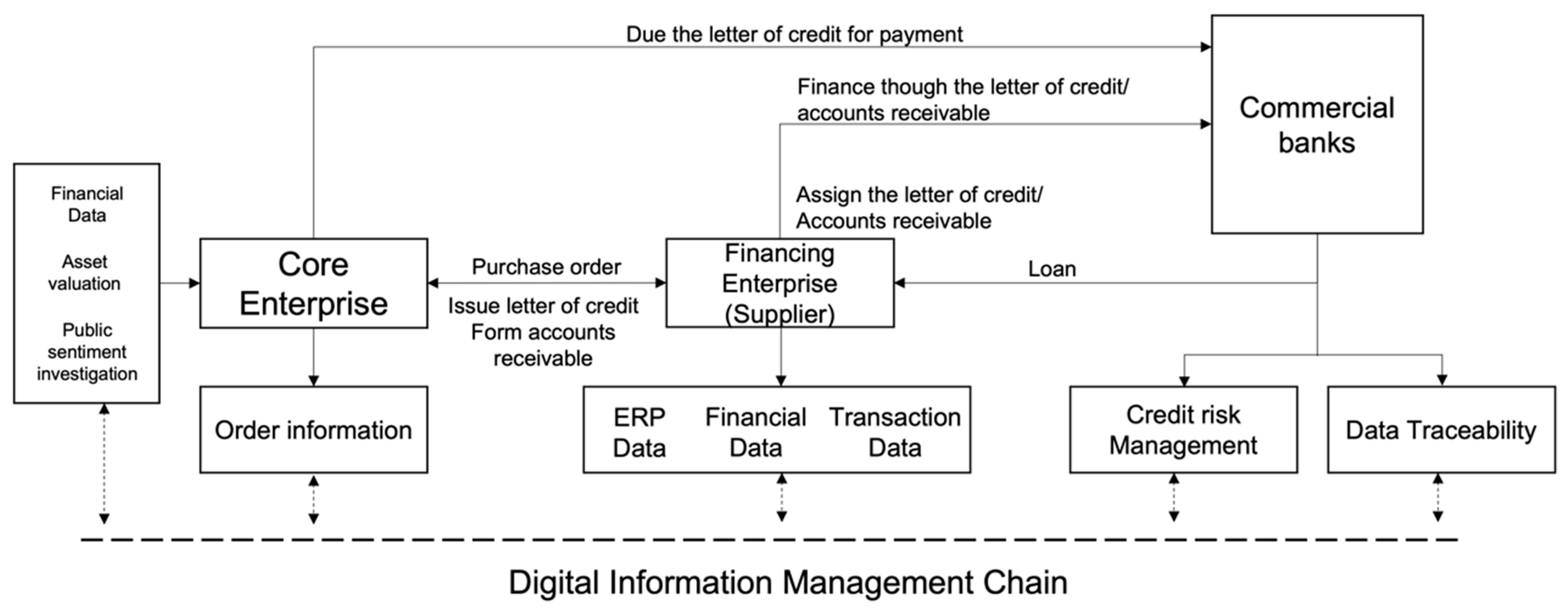
Compared to traditional SCF, an important feature of DSCF is the “enterprise data on the chain”, i.e., the enterprises in the supply chain register and confirming their transaction information on the chain (see Figure 1), which is a different way of digitizing enterprises than the internet (Goldfarb and Tucker [25]). For the realization of this feature, the digitalization of both financial institutions and enterprises is essential, with the digitalization of enterprises also playing an important role in the risk control of SCF. Firstly, the information recording, IoT technology, plays a role in collecting and recording information, warehouse management system (WMS), supplier relationship management (SRM), customer relationship management (CRM), etc., which are all supply chain information collection and recording systems. Secondly, the dissemination of information, in digital form, makes it possible to share, collaborate, and monitor information in real-time across locations. Enterprise resource planning (ERP), for example, is called the internal information internet of the enterprise. Thirdly, information processing, i.e., the fast and accurate processing of information, e.g., advanced planning and scheduling (APS) is an information processing system for the supply chain management. The new generation platform features intelligent multi-party connection, mutual trust of chain enterprises, multi-level credit penetration and closed-loop ecological risk control, which is expected to drive the development of enterprise financing business in relatively risk-controlled batches by transferring core enterprise credit at multiple levels and closing the loop of funds in an operational manner.

2.2. Machine Learning and Credit Risk Models

The issue of credit risk assessment in SCF has attracted the attention of scholars. Hallikas et al. [26] used internal audit and computer cameras and analyzed the causes of risk through interviews with two core enterprises and nine suppliers, and classified the risks of SCF into four parts: demand, transaction, pricing, and finance. Finch [27] analyzed the literature on the need for core firms to determine whether to use SMEs as a supply partner for critical operations and to establish appropriate information systems for review, and found that improved information management of SMEs contributed to credit risk reduction. Yurdakul and İç [28] developed a credit assessment and decision-making model for determining the credibility of manufacturing firms. Ghadge et al. [29] developed a holistic, systematic, and quantitative risk assessment process to measure overall risk behavior. By capturing dynamic risks in case studies of manufacturing firms, the overall risk impact of SCF can be predicted and a whole picture of risk behavior exhibited is constructed. With the gradual improvement of SCF applications, the credit risks they face are becoming increasingly complex. Subjective assessments based on experience and traditional linear models are no longer able to accurately predict risks, and assessment models based on machine learning techniques are now more popular. Many research results have been achieved in the assessment of enterprise credit risks in SCF. Zhu et al. [30] used an integrated ensemble machine learning approach to assess SME credit risk in Chinese SCF. The RS-boosting method was found to outperform other methods in improving the accuracy of risk prediction. Zhu et al. [31] further used a new hybrid ensemble machine learning method, RS-MultiBoosting, which improved the accuracy of credit risk assessment based on the SCF in China. Wang et al. [10] then explored the mechanism of online SCF using least squares support vector machine (LS-SVM) method and found that LS-SVM method has higher accuracy in online SCF risk prediction.

Due to the complexity of credit risk, there are various models for credit risk assessment, which have undergone a series of improvements since their development. Prior to 1970, financial institutions such as commercial banks mainly carried out qualitative analysis of financing companies by professionals and credit assessment was more subjective. The methods used included expert scoring and profiling. After 1970, financial institutions used ZETA scoring models, Z-score models, and other statistical distributions to assess the credit risk of financing companies. Orgler [32] studied credit risk based on the characteristics of linear regression, and later linear regression methods also provided many references to credit risk assessment problems (Fitzpatrick [33]; Lucas [34]; Henley [35]). However, in view of the shortcomings of linear discriminatory methods, non-linear statistical models such as logistic regression (LR) and Probit have emerged as commonly used models for multivariate credit risk assessment. Wiginton [36] assessed risk on the basis that logistic regression can explain problems where the variable is a qualitative indicator, and Steenackers and Goovaens [37] made a related follow-up application of personal loans. Cramer [38] systematically investigated LR and showed that LR was more accurate in classification, and that its low assumptions and high stability made it one of the most widely used methods for credit risk assessment. Profit regression was used by Grablowsky and Talley [39] in their study of credit risk and the results showed that profit regression did not have as good an interpretation as LR.

Further, the classification tree method was first applied to credit risk assessment by Makowsik [40], whose results were compared and which confirmed its high accuracy in credit assessment applications, with the advantage of automatic variable selection and better handling of missing information (Carter and Catlett [41]). While Cover [42] proposed the k-nearest neighbor (KNN) discriminant method, and then Henley et al. [43] applied the KNN analysis method to personal credit assessment and confirmed the feasibility of KNN in credit risk assessment. Hand [44] used the KNN method and decision trees (DT) to identify loan risk, and the results showed that the KNN method had better prediction accuracy. Subsequently, Bayesian algorithms were proposed by Pearl [45] and have been used to good effect in the areas of representation of uncertain knowledge and inference. The research of Hsieh [46] showed that Bayesian networks enable to intuitively represent the relationship between attributes and probabilities, and have good explanatory power. As Bayesian classification models combine prior knowledge and sample information and use probability tables to quantify the dependencies between variables with better classification accuracy, they have attracted increasing attention from scholars. The naïve Bayesian (NB) classification algorithm (Friedman et al. [47]), a milestone in Bayesian classification research, assumes that all feature variables are independent of each other where the class node is the parent of all attribute nodes in the structured graph, with no arcs between any other attribute nodes. A good classification with a simple structure can be obtained using an NB classifier when the correlation between feature variables is small, but its strict conditional independence is often not achieved under realistic conditions thereby greatly reducing its classification effectiveness (Langley et al. [48]).

As the application of machine learning methods in credit risk assessment continues to evolve, do Prado et al. [49] used the Web Science database to analyze the journal literature on credit risk and bankruptcy research published between 1968 and 2014 using bibliometric methods. They found that LR has been a common approach though, since Odom and Sharda [50] first used Artificial Neural Network (ANN) for credit risk assessment, artificial intelligence (AI) techniques represented by neural networks have been used more and more widely, and multiple or hybrid models with sophisticated AI techniques are a trend for further research. Since credit risk assessment models based on AI techniques do not require strict assumptions to be made and have advantages in dealing with non-linear problems (Denison et al. [6]), they have become more popular when facing increasingly complex credit risk. Davis et al. [51] conducted a case study of neural networks in personal credit assessment and found that the neural network method was more accurate in classification, but the training time for the neural network data was longer. Desai et al. [52] also used neural networks in personal credit assessment and showed that their performance was better. Piramuthu [53] developed a neural network survival model using multi-layer perceptron (MLP) neural networks and fuzzy neural network-related principles. Lee and Chen [54] used neural networks and the related theory of multivariate adaptive spline regression to investigate the feasibility of applying the related theory to credit assessment. Tsai [55] applied the principles of MLP neural networks to corporate bankruptcy prediction and credit assessment. Marcano-Cedeño et al. [56] developed a plasticity neural network model and then conducted an empirical study using relevant data. Coincidently, the theory of support vector machine (SVM) was first proposed by Cortes and Vapnik [57] in 1995, and SVM has quickly become a hot topic of research in machine learning in recent years. Stecking and Schebesch [58] selected different kernel functions and then analyzed the impact of these kernel functions on credit appraisal. Lai et al. [59] modeled the problem of credit assessment and verified the feasibility of the theory in credit assessment by using the theory related to least squares support vector machines. Schebesch and Stecking [60] developed a credit assessment model by combining these principles through a study of combined support vector machines and imbalanced data sets. Yu et al. [61] developed a credit risk assessment model based on hybrid intelligent mining, in which rough set theory and the related theory of support vector machines were used.

Controversy surrounds the choice of credit risk assessment models. The advent of SVM has provided excellent algorithms for classification models, with a large number of kernel functions available for flexible solutions to a wide range of non-linear classification regression problems. However, model selection is also the main problem with SVMs, as the selection of kernels and the optimization of kernels and regularization parameters can often lead to severe overfitting if the model selection criteria are over-optimized, while the emergence of ANNs has effectively bridged the shortcomings of traditional methods. ANNs are widely used for the estimation and prognosis of complex processes due to their ability to classify research populations in complex environments using large amounts of uncertain information. The advantage of ANNs is that they do not require a strict distribution of the data, nor do they require a detailed representation of the function between the independent and dependent variables, and they are effective in solving non-normally distributed non-linear credit assessment problems. However, neural networks also have their disadvantages, namely the long training time and the difficulty in identifying the relative importance of the input variables in order to obtain the optimal network. Among the ANNs, MLP neural networks have been used in risk assessment due to their outstanding performance.

3. Methodology

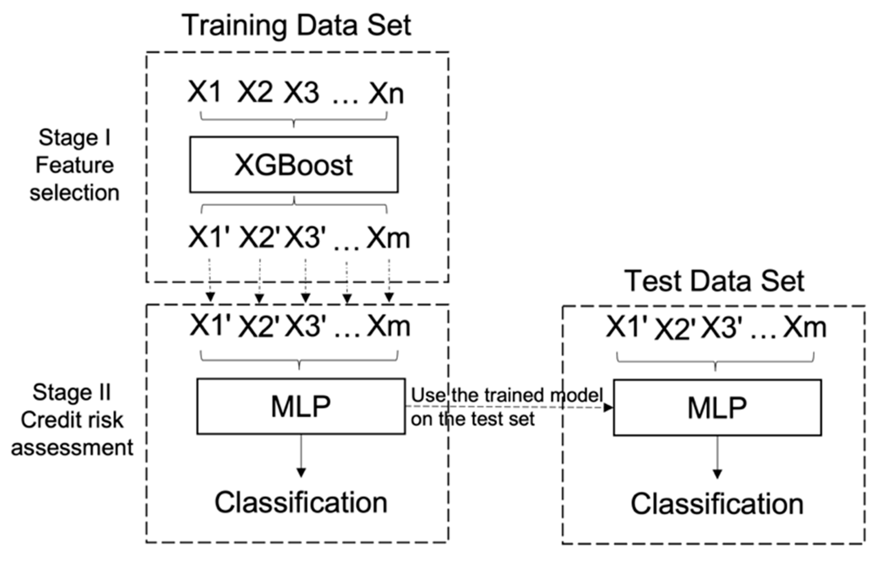
In order to accurately and effectively conduct a credit risk assessment, we construct the following model (See Figure 2). In the first stage, through feature selection, we extract the training sample set and select the features with higher scores based on the importance score of the calculated features. In the second stage, MLP is used for credit risk assessment based on the selected features. As credit risk assessment can essentially be seen as a classification problem, the MLP is used as a classification model in the credit assessment process. Further, the trained model is used to test the test set and ultimately, we validate the proposed research question. Specifically, given the training set $\mathit{X}$, ${\mathit{x}}_{\mathit{i}}$ represents the original features as the input of credit risk assessment and ${\mathit{y}}_{\mathit{i}}$ is the label of credit status ($\mathit{Y}=\mathbf{0} \mathit{o}\mathit{r} \mathbf{1}$, i.e., risky/non-risky). $\mathit{X}=\{\left({\mathit{x}}_{\mathbf{1}},{\mathit{y}}_{\mathbf{1}}\right), \left({\mathit{x}}_{\mathbf{2}},{\mathit{y}}_{\mathbf{2}}\right),\dots ,({\mathit{x}}_{\mathit{n}},{\mathit{y}}_{\mathit{n}})\}$. Based on the importance ranking ${\mathit{r}}_{\mathit{n}}$ by XGBoost classifier in the first stage, we filter the features by thresholds ${\mathit{t}}_{\mathit{i}}$ and remove features ${\mathit{x}}_{\mathit{n}}$ where ${\mathit{r}}_{\mathit{n}}<{\mathit{t}}_{\mathit{i}}$. Then we obtain the remained features in subset ${\mathit{X}}^{\mathbf{\prime }}$ as the input for retraining with MLP. Though the $\mathit{R}\mathit{e}\mathit{L}\mathit{U}$-based MLP, $\mathit{R}\mathit{e}\mathit{L}\mathit{U}$ as the activation function is more expressive for linear functions. For non-linear functions, $\mathit{R}\mathit{e}\mathit{L}\mathit{U}$ does not have the vanishing gradient problem as the gradient of the non-negative interval is constant, allowing the convergence rate of the model to be maintained in a steady-state. Thus, we obtain the output of $\mathit{y}=\mathit{f}\left(\mathit{x}\right)=\mathbf{max}\left(\mathbf{0},\mathit{x}\right)$ and the performance of the model.

3.1. Stage I: Feature Selection with XGBoost

XGBoost is an improved algorithm based on Gradient Boosting Decision Trees (GBDT) proposed by Chen and Guestrin [62], which can efficiently build augmented trees and run in parallel. This is an ensemble learning method where the basic idea is to select some samples and features to generate a simple model (e.g., a decision tree) as the basic classifier and to learn the residuals of the previous model, minimize the target function, and generate a new model, which is repeated to produce a combination of hundreds of linear or tree models with high accuracy. At its core, the new model is built in the direction of the corresponding gradient of the loss function, correcting for residuals while controlling complexity. Thus, the dataset in our paper containing $\mathit{n}$ examples with $\mathit{e}$ features is denoted as $\mathit{X}=\left\{\left({\mathit{x}}_{\mathit{i}},{\mathit{y}}_{\mathit{i}}\right):{\mathit{x}}_{\mathit{i}}\in {\mathit{R}}^{\mathit{e}}, {\mathit{y}}_{\mathit{i}}\in \mathit{R}, \left|\mathit{X}\right|=\mathit{n}\right\}$, and the set of all classification and regression trees (CART) [63] is denoted as $\mathit{F}=\left\{\mathit{f}\left(\mathit{x}\right)={\mathit{w}}_{\mathit{q}\left(\mathit{x}\right)}, \mathit{q}:{\mathit{R}}^{\mathit{e}}\to \mathit{T}, \mathit{w}\in {\mathit{R}}^{\mathit{T}}\right\}$ where $\mathit{q}$ is the rule structure for mapping the samples to the corresponding leaf nodes, $\mathit{T}$ is the number of leaf nodes in a tree, and $\mathit{w}$ is the weight of the leaf nodes. $\mathit{f}$ represents the CART, including the structure of the tree $\mathit{q}$ and the weight of the leaf nodes $\mathit{w}$. CART decision trees are divided into regression trees and classification trees, and CART regression trees, which assume that a DT is a binary tree. It constructs a DT by continuously splitting the features (into left and right halves). The predicted value of ${\mathit{y}}_{\mathit{i}}$ based on the XGBoost algorithm can be expressed as:

$${\widehat{\mathit{y}}}_{\mathit{i}}=\mathit{\theta }\left({\mathit{x}}_{\mathit{i}}\right)={{\displaystyle \sum }}_{\mathit{k}=\mathbf{1}}^{\mathit{K}}{\mathit{f}}_{\mathit{k}}\left({\mathit{x}}_{\mathit{i}}\right)$$

(1)

where ${\mathit{f}}_{\mathit{k}}\in \mathit{F}$ and $\mathit{K}$ is the number of CART. ${\mathit{f}}_{\mathit{k}}\left(\mathit{x}\right)$ represents a DT, that function $\mathit{f}$ can be interpreted as mapping the sample $\mathit{x}$ into some leaf node of the tree, and each leaf node in the tree will correspond to a weight $\mathit{w}$.

We consider a general objective function first:

$$\mathit{o}\mathit{b}\mathit{j}\left(\mathit{\theta }\right)={\displaystyle \sum }_{\mathit{i}}\mathit{l}\left({\widehat{\mathit{y}}}_{\mathit{i}},{\mathit{y}}_{\mathit{i}}\right)+{\displaystyle \sum }_{\mathit{k}}\Omega \left({\mathit{f}}_{\mathit{k}}\right)$$

(2)

$$\Omega \left(\mathit{f}\right)=\mathit{\gamma }\mathit{T}+\frac{\mathbf{1}}{\mathbf{2}}\mathit{\lambda }{\left|\right|\mathit{w}\left|\right|}^{\mathbf{2}}$$

(3)

Among them, $\mathit{l}$ is a derivable and convex loss function, which is used to measure the similarity between $\widehat{\mathit{y}}$ and $\mathit{y}$. The second term $\Omega$ is a regular term, which contains two parts. The first one is $\mathit{\gamma }\mathit{T}$, where $\mathit{T}$ is leaf. The number of nodes, $\mathit{\gamma }$, is a hyperparameter that if $\mathit{\gamma }$ is larger, the number of leaf nodes will be smaller. The other part is the L2 regularization term, which penalizes the weight of the leaf nodes so that there will be no leaf nodes with too large weights to prevent overfitting.

It is difficult to optimize and minimize the above objective function Equation (2), so we transform it by greedily optimizing the objective function by adding a base classifier ${\mathit{f}}_{\mathit{t}}$ at each step, so that each time it is added, the loss becomes smaller. In this way, we obtain an evaluation function that can be used to evaluate the performance of the current classifier ${\mathit{f}}_{\mathit{t}}$.

$$\mathit{o}\mathit{b}\mathit{j}\left(\mathit{t}\right)={\displaystyle \sum }_{\mathit{i}=\mathbf{1}}^{\mathit{n}}\mathit{l}\left({\mathit{y}}_{\mathit{i}}, {\widehat{\mathit{y}}}_{\mathit{i}}^{\left(\mathit{t}-\mathbf{1}\right)}+{\mathit{f}}_{\mathit{t}}\left({\mathit{x}}_{\mathit{i}}\right)\right)+\Omega \left({\mathit{f}}_{\mathit{t}}\right)$$

(4)

where ${\mathit{y}}_{\mathit{i}}$ is the $\mathit{i}$ target and ${\widehat{\mathit{y}}}_{\mathit{i}}^{\mathit{t}}={\widehat{\mathit{y}}}_{\mathit{i}}^{\left(\mathit{t}-\mathbf{1}\right)}+{\mathit{f}}_{\mathit{t}}\left({\mathit{x}}_{\mathit{i}}\right)$ is the prediction for the $\mathit{t}$th iteration. Equation (4) can also be called forward stepwise optimization. To optimize this function more quickly, we do a second-order Taylor expansion at ${\mathit{f}}_{\mathit{t}}=\mathbf{0}$.

$$\mathit{o}\mathit{b}\mathit{j}\left(\mathit{t}\right)\approx {\displaystyle \sum }_{\mathit{i}=\mathbf{1}}^{\mathit{n}}\left[\mathit{l}\left({\mathit{y}}_{\mathit{i}}, {\widehat{\mathit{y}}}^{\left(\mathit{t}-\mathbf{1}\right)}\right)+{\mathit{g}}_{\mathit{i}}{\mathit{f}}_{\mathit{t}}\left({\mathit{x}}_{\mathit{i}}\right)+\frac{\mathbf{1}}{\mathbf{2}}{\mathit{h}}_{\mathit{i}}{\mathit{f}}_{\mathit{t}}^{\mathbf{2}}\left({\mathit{x}}_{\mathit{i}}\right)\right]+\mathit{\gamma }\mathit{T}+\Omega \left({\mathit{f}}_{\mathit{t}}\right)$$

(5)

where ${\mathit{g}}_{\mathit{i}}$ denotes the first order partial derivative of $\mathit{l}$ with respect to $\mathit{f}$ and ${\mathit{h}}_{\mathit{i}}$ denotes the second order partial derivative of $\mathit{l}$ with respect to $\mathit{f}$.

$${\mathit{g}}_{\mathit{i}}={\mathit{\partial }}_{{\widehat{\mathit{y}}}_{\mathit{i}}^{\left(\mathit{t}-\mathbf{1}\right)}}\mathit{l}\left({\mathit{y}}_{\mathit{i}}, {\widehat{\mathit{y}}}_{\mathit{i}}^{\left(\mathit{t}-\mathbf{1}\right)}\right)$$

(6)

$${\mathit{h}}_{\mathit{i}}={\partial }_{{\widehat{\mathit{y}}}_{\mathit{i}}^{\left(\mathit{t}-\mathbf{1}\right)}}^{\mathbf{2}}\mathit{l}\left({\mathit{y}}_{\mathit{i}}, {\widehat{\mathit{y}}}_{\mathit{i}}^{\left(\mathit{t}-\mathbf{1}\right)}\right)$$

(7)

Then we define the total number of samples as $\mathit{n}$, each sample as $\mathit{i}$, the information of $\mathit{i}$ is divided into some leaf node information, and define the weight of each leaf belonging to $\mathit{i}$ as $\mathit{j}$. ${\mathit{I}}_{\mathit{j}}=\left\{\mathit{i}\right|\mathit{q}\left({\mathit{x}}_{\mathit{i}}\right)=\mathit{j}\}$ is the instance set of leaf $\mathit{i}$.

$$\begin{gathered} \widetilde{\mathit{o}\mathit{b}\mathit{J}}\left(\mathit{t}\right)={\displaystyle \sum }_{\mathit{i}=\mathbf{1}}^{\mathit{n}}\left[{\mathit{g}}_{\mathit{i}}{\mathit{f}}_{\mathit{t}}\left({\mathit{x}}_{\mathit{i}}\right)+\frac{\mathbf{1}}{\mathbf{2}}{\mathit{h}}_{\mathit{i}}{\mathit{f}}_{\mathit{t}}^{\mathbf{2}}\left({\mathit{x}}_{\mathit{i}}\right)\right]+\mathit{\gamma }\mathit{T}+\frac{\mathbf{1}}{\mathbf{2}}\mathit{\lambda }{\displaystyle \sum }_{\mathit{j}=\mathbf{1}}^{\mathit{T}}{\mathit{w}}_{\mathit{j}}^{\mathbf{2}} \\ ={\displaystyle \sum }_{\mathit{j}=\mathbf{1}}^{\mathit{n}}\left[\left({\displaystyle \sum }_{\mathit{i}\in {\mathit{I}}_{\mathit{j}}}{\mathit{g}}_{\mathit{i}}\right){\mathit{w}}_{\mathit{j}}+\frac{\mathbf{1}}{\mathbf{2}}\left({\displaystyle \sum }_{\mathit{i}\in {\mathit{I}}_{\mathit{j}}}{\mathit{h}}_{\mathit{i}}+\mathit{\lambda }\right){\mathit{w}}_{\mathit{j}}^{\mathbf{2}}\right]+\mathit{\gamma }\mathit{T} \end{gathered}$$

(8)

Define the ${\mathit{G}}_{\mathit{i}}=\sum _{\mathit{i}\in {\mathit{I}}_{\mathit{j}}}{\mathit{g}}_{\mathit{i}}$, ${\mathit{H}}_{\mathit{i}}=\sum _{\mathit{i}\in {\mathit{I}}_{\mathit{j}}}{\mathit{h}}_{\mathit{i}}$, then let the current function derivative of $\mathit{w}$ be 0. At this point, the objective function becomes quadratic with respect to $\mathit{w}$. The optimal weight for the fixed $\mathit{q}\left(x\right)$ is:

$${\mathit{w}}_{\mathit{j}}^{*}=\frac{{\mathit{G}}_{\mathit{j}}}{{\mathit{H}}_{\mathit{j}}+\mathit{\lambda }}$$

(9)

Substituting Equation (9) into the objective function gives:

$${\widetilde{\mathit{o}\mathit{b}\mathit{J}}}^{*}=-\frac{\mathbf{1}}{\mathbf{2}}{\displaystyle \sum }_{\mathit{j}=\mathbf{1}}^{\mathit{T}}\frac{{\mathit{G}}_{\mathit{j}}^{\mathbf{2}}}{{\mathit{H}}_{\mathit{j}}+\mathit{\lambda }}+\mathit{\gamma }\mathit{T}$$

(10)

When selecting features for XGBoost-based classification, feature importance is integrated into the classification process. A new tree is created in each iteration, and the branch nodes in the tree are a feature variable, and the importance of these nodes is calculated. The importance of a feature is based on the squared improvement of the split nodes of the tree that a feature is selected for. Each time a feature is selected to be added to the tree as a splitting node, all possible splitting points are enumerated using a greedy algorithm, from which the splitting point with the best gain is selected. The best splitting point corresponds to the maximum gain, and the gain is calculated by the formula:

$${\mathit{G}}_{\mathit{a}\mathit{i}\mathit{n}}=\frac{\mathbf{1}}{\mathbf{2}}\left[\frac{{\mathit{G}}_{\mathit{L}}^{\mathbf{2}}}{{\mathit{H}}_{\mathit{L}}+\mathit{\lambda }}+\frac{{\mathit{G}}_{\mathit{R}}^{\mathbf{2}}}{{\mathit{H}}_{\mathit{R}}+\mathit{\lambda }}-\frac{{\left({\mathit{G}}_{\mathit{L}}+{\mathit{G}}_{\mathit{R}}\right)}^{\mathbf{2}}}{{\mathit{H}}_{\mathit{L}}+{\mathit{H}}_{\mathit{R}}+\mathit{\lambda }}\right]-\mathit{\gamma }$$

(11)

where the ${\mathit{I}}_{\mathit{L}}$ and ${\mathit{I}}_{\mathit{R}}$ are the instance sets of left and right nodes after splitting. Relevant features and split points improve the squared difference on a single tree, and the more improvement there is, the better the split point and the more important the feature is. When all trees are built, the calculated node importance is averaged over the forest. The more times a feature is selected as a split point, the more important it will be.

3.2. Stage II: Credit Risk Assessment Models

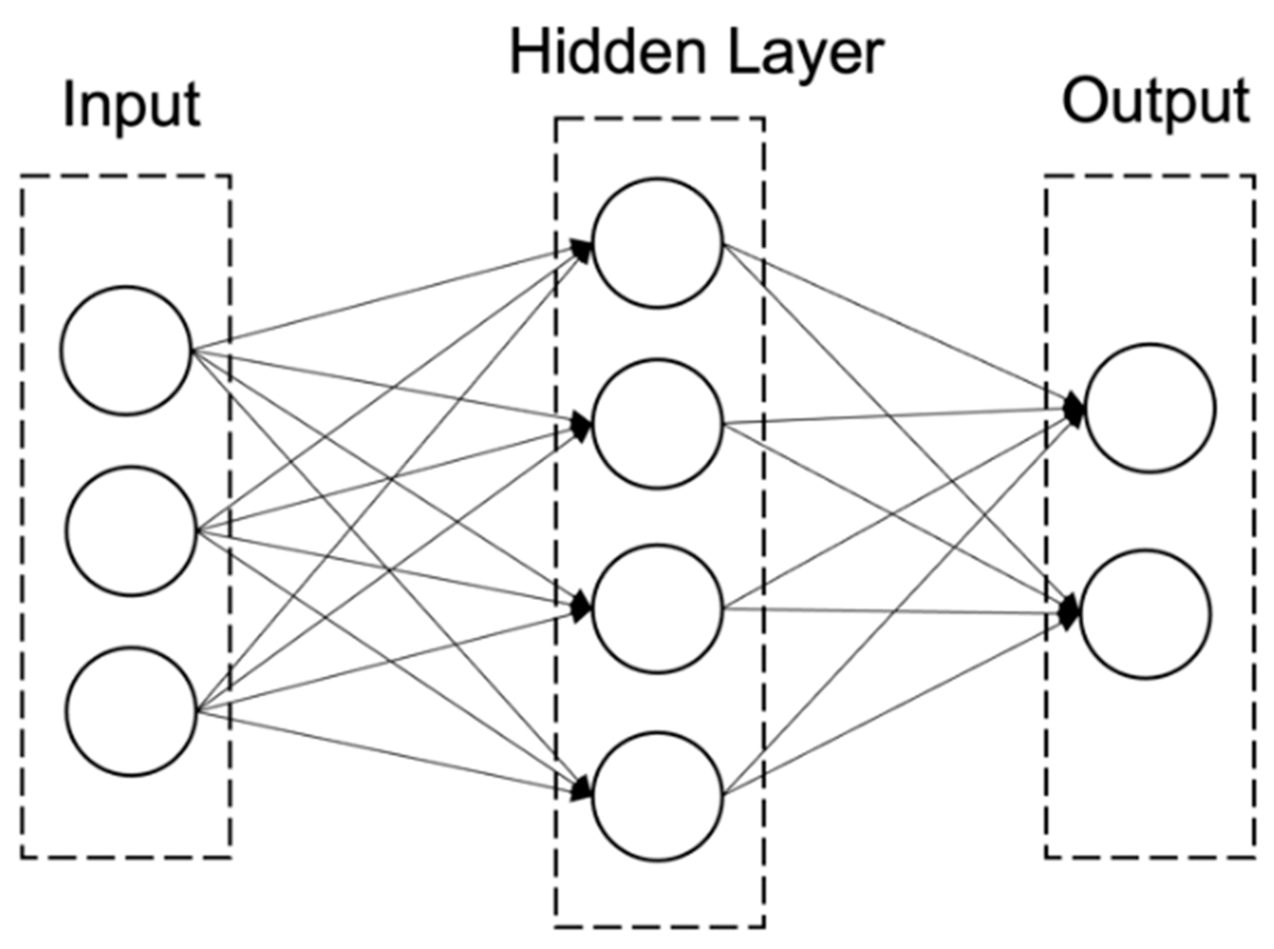
As part of the second stage, we utilize several models, namely a MLP, KNN, NB, DT, RF, and SVM. MLP, an ANN with forwarding agency that maps a set of input vectors to a set of output vectors, is thought of as a directed graph, consisting of multiple layers of nodes, each layer fully connected to the next (see Figure 3). In addition to the input nodes, each node is a neuron (or processing unit) with a non-linear activation function. A supervised learning method known as backpropagation is often used to train MLPs, which overcomes the weakness of the perceptron in their inability to recognize non-linear data. MLP has been shown to be a general function approximation method that can be used to fit complex functions or to solve classification problems. For more details on MLPs and their modeling design, we refer the interested reader to Sermpinis et al. [64].

The LR model is widely used in corporate credit risk assessment research, and the LR model is used to calculate the relationship between the dependent variables and the independent variables as well as the strength of the relationship (Crook et al. [65]). In this paper, the subject of credit risk research, i.e., enterprise in the digital supply chain financial environment, is divided into two categories: one category is risky SMEs; the other category is non-risky enterprises, and the binary LR method is used to assess the credit risk based on the DSCF environment. For more details on LRs and their modeling design, we refer the interested reader to Hassanniakalager et al. [66]. KNN is a non-parametric estimation method in the field of pattern recognition (Cover and Hart [67]). The algorithm is simple, fast and efficient, and the idea is to assume that a sample data $\mathit{x}$ is to be recognized, where most of the $\mathit{k}$-nearest-neighbor training sample representative points in the feature space belong to one of the categories, then $\mathit{x}$ also belongs to this category. The Euclidean distance is generally used to measure the distance between the sample with the training sample. For more details on KNNs and their modeling design, we refer the interested reader to Sermpinis et al. [68].

The NB classifier is the simplest Bayesian classifier with the advantage of high efficiency and good classification accuracy (Rish [69]; Antonakis and Sfakianakis [70]). In its structure, the class variables are treated as parents of the other attribute variables, and it is assumed that the attribute variables are independent of each other, provided that the class variables are known. For more details on NBs and their modeling design, we refer the interested reader to Hassanniakalager et al. [71]. The DT algorithm is a binary tree decision method similar to that used in risk management theory and a conditional branching structure in discrete mathematical flowchart theory, where probability calculations are used to classify the categories (Breiman et al. [63]). The DT model makes an inductive classification algorithm that learns from a sample of training data, and then suitable decision rules are then used to analyze the test data samples. The DT algorithm divides the data into subsets depending on whether the selected attribute is discrete or numerical. The corresponding subsets are then divided recursively until the division is no longer required and a leaf node is placed to identify it. There are many classification algorithms for DTs, including the Iterative Dichotomiser 3 (ID3) algorithm and the C 4.5 algorithm proposed by Quinlan [72].

The RF method is a classification model based on DT theory, but which differs from DT in that the RF does not generate only unique trees, and randomly uses variables and data in the process of generating DTs (Breiman [73]). It is also known as a random DT because it uses variables and data randomly in the process of generating a DT that contains multiple DTs. RF contains the idea of integrated learning, which means that weak classifiers are learned and trained to combine into strong classifiers. In the RF model, this integrated learning theory is based on the Bagging algorithm (Bootstrap aggregating). The difference is that the RF model creates a DT by splitting the set of attributes for random selection. SVM is the linear classifier first proposed by Cortes and Vapnik [57]. The SVM has advantages in solving small-sample, non-linear and high-dimensional pattern recognition (Cusano et al. [74]). For non-linear problems, a non-linear transformation $\mathit{f}\left(\mathit{x}\right)$ is used to map the input data into a high-dimensional feature space, and then go for linear classification in the high-dimensional feature space, which solves the low-dimensional space (Bao et al. [75]). The linearly indivisible problem in low-dimensional space could be transformed into a linearly divisible problem in high-dimensional feature space by Kernel function, basically including linear, polynemoid, radial bias function, and sigmoid. For more details on SVM and their modeling design for classification or regression tasks, we refer the interested reader to Stasinakis et al. [76].

4. Experimental Design

In order to compare the performance of the XGBoost-MLP model with other traditional models for credit risk assessment of DSCF, we selected listed SMEs in China as our data sample because SMEs in China are a major demand-side of SCF which is certainly representative. The studies on SCF in China are relatively limited, and it is difficult to collect relevant data. Thus, we firstly select listed SMEs as the main subject of the credit risk assessment, which represents the main target of supply chain financial services. Secondly, large enterprises listed on the Main Board are selected as the core enterprises, which have the strong financial strength and enable them to act as important guarantors in the supply chain. The requirements for listing on the Main Board are the highest, with the listing criteria requiring the company to be established and in operation for at least three years, and to be profitable for three years, with an aggregate of more than RMB 30 million, and the company’s net cash flow from operations for three years to exceed an aggregate of RMB 50 million. The company is also required to have a cumulative total of more than RMB 300 million over three years, plus a total pre-issue share capital of not less than RMB 30 million. Companies that can successfully list on the Main Board are in a leading position in a certain industry (https://www.szse.cn/English/products/equity/mainboards/index.html, accessed on 5 February 2021). Thirdly, the selected SMEs have real trading relationships with the core enterprises, and they are suppliers or customers of the core enterprises. Based on the above selection criteria, we selected 85 listed SMEs from 31 March 2016–31 December 2019 from the Small and Medium Enterprise Board of the Shenzhen and Shanghai Stock Exchange including a quarterly 1357-observations dataset of risky and non-risky enterprises.

All companies selected are private manufacturing companies that have been listed for more than 10 years. Although this method of data collection is commonly used in the existing literature (Zhang et al. [77]; Zhu et al. [31]; Zhu et al. [30]), it has certain limitations that make the results susceptible to error. Hence, certain improvements have been made on this basis. Firstly, most of the relevant data samples are collected through questionnaires on non-financial data related to the supply chains which is somewhat subjective and arbitrary, and can bias the experimental results. Thus, we use publicly available financial data for the SCF part of the feature data to be measured. Secondly, the existing literature mostly takes SCF or online SCF as the research object, and there are gaps in research on the characteristics of the DSCF. In this paper, through the analysis and investigation of DSCF, digital features are added to the credit risk assessment. Thirdly, there are few data treatments in the existing literature that focus on feature selection. Zhu et al. [30] use the DT to evaluate data samples and derive important rankings before conducting classification assessment. Although the algorithm of DT is simple and interpretable, the risk of overfitting is great and the application scenario is limited. In this paper, we use XGBoost as the first stage feature selection method, which improves on the basis of GBDT by adding a regular term to the objective function of each iteration to further reduce the risk of overfitting, thus improving the performance for feature selection.

The 85 listed SMEs comprise 11 enterprises under special treatment under risk alert, i.e., ST and *ST stocks, which are regarded as risky SMEs with negative credit status, and 74 enterprises with normal financial status. Thus, we classify the dependent variables into two groups based on the credit status; the dependent variables are assigned the value of 0 or 1 which indicates the risky and non-risky enterprises. We select 30% of the data set as the test set, i.e., 408 observations, with 49 negative examples and 359 positive examples, and 949 observations in the training set, with 127 negative examples and 822 positive examples.

In addition, the confusion matrix and its derived assessment metrics are used to evaluate the results of the sample data. In this paper, positive samples are creditworthy, i.e., risk-free firms, and negative samples are bad creditworthy, i.e., risky firms. The parameters mentioned below are calculated based on a confusion matrix shown in

Table 1. Confusion matrix.

		Actual Condition
		Positive (non-risky)	Negative (risky)
Test result	Positive (non-risky)	True positive (TP)	False positive (FP)
	Negative (risky)	False negative (FN)	True negative (TN)

. True positive (TP) refers to the number of defaults that are correctly predicted as defaults; false positive (FP) refers to the number of non-defaults that are mistakenly predicted as defaults; true negative (TN) refers to the number of non-defaults that are correctly predicted as non-default; false negative (FN) refers to the number of defaults that are mistakenly predicted as non-defaults. The parameters used in this work are calculated with the following equations (Equations (12)–(18)).

The accuracy rate represents the proportion of correct samples to the total sample:

$$\mathit{A}\mathit{v}\mathit{e}\mathit{r}\mathit{a}\mathit{g}\mathit{e} \mathit{A}\mathit{c}\mathit{c}\mathit{u}\mathit{r}\mathit{a}\mathit{c}\mathit{y}=\frac{\mathit{T}\mathit{P}+\mathit{T}\mathit{N}}{\mathit{T}\mathit{P}+\mathit{F}\mathit{P}+\mathit{T}\mathit{N}+\mathit{F}\mathit{N}}$$

(12)

Precision indicates the number of samples that are predicted to be positive that are truly positive and recall indicates the number of positive cases in the sample that was correctly predicted. Precision is specific to the predicted output and recall is specific to the original sample. Type I error is defined as the number of true negative samples incorrectly predicted to be positive as a proportion of the number of all true negative samples; while Type II error is defined as the number of true positive samples incorrectly predicted to be negative as a proportion of the number of all true positive samples.

$$\mathit{P}\mathit{r}\mathit{e}\mathit{c}\mathit{i}\mathit{s}\mathit{i}\mathit{o}\mathit{n}=\frac{\mathit{F}\mathit{P}}{\mathit{T}\mathit{P}+\mathit{F}\mathit{P}}$$

(13)

$$\mathit{R}\mathit{e}\mathit{c}\mathit{a}\mathit{l}\mathit{l}=\frac{\mathit{T}\mathit{P}}{\mathit{T}\mathit{P}+\mathit{F}\mathit{N}}$$

(14)

$$\mathit{T}\mathit{y}\mathit{p}\mathit{e} \mathit{I} \mathit{E}\mathit{r}\mathit{r}\mathit{o}\mathit{r}=\frac{\mathit{F}\mathit{P}}{\mathit{T}\mathit{P}+\mathit{F}\mathit{N}}$$

(15)

$$\mathit{T}\mathit{y}\mathit{p}\mathit{e} \mathit{I}\mathit{I} \mathit{E}\mathit{r}\mathit{r}\mathit{o}\mathit{r}=\frac{\mathit{F}\mathit{N}}{\mathit{T}\mathit{N}+\mathit{F}\mathit{P}}$$

(16)

The F-Measure is the composite index based on the accuracy and recall; the closer the F-Measure is to 1, the better the classification model is.

$$\mathit{F}-\mathit{M}\mathit{e}\mathit{a}\mathit{s}\mathit{u}\mathit{r}\mathit{e}=\frac{\mathbf{2}\times \mathit{T}\mathit{P}}{\mathbf{2}\times \mathit{T}\mathit{P}+\mathit{F}\mathit{P}+\mathit{F}\mathit{N}}$$

(17)

The Matthew correlation coefficient (MCC) takes into account true and false positives and false negatives, and is often seen as an unbalanced measure that can be used even if these categories are of different sizes.

MCC is essentially the correlation coefficient between the observed category and the predicted binary category; it returns a value between −1 and +1. A coefficient of +1 indicates a perfect prediction, 0 indicates no better than a random prediction, and −1 indicates a complete inconsistency between prediction and observation.

$$\mathit{M}\mathit{C}\mathit{C}=\frac{\left(\mathit{T}\mathit{P}\ast \mathit{T}\mathit{N}\right)-\left(\mathit{F}\mathit{P}\ast \mathit{F}\mathit{N}\right)}{\sqrt{\left(\mathit{T}\mathit{P}+\mathit{F}\mathit{P}\right)\left(\mathit{T}\mathit{P}+\mathit{F}\mathit{N}\right)\left(\mathit{T}\mathit{N}+\mathit{F}\mathit{P}\right)\left(\mathit{T}\mathit{N}+\mathit{F}\mathit{N}\right)}}$$

(18)

5. Experimental Result

Following the existing literature (Zhu et al. [31]; Wang and Ma [78]; Wang et al. [10]), 17 independent variables are selected.

Table 2. Variables for enterprise credit risk analysis.

Groups	Independent Variables
Status of financing company	Current ratio of SMEs
	Quick ratio of SMEs
	Working capital turnover of SMEs
	Accounts receivable turnover ratio of SMEs
	Rate of return on total assets of SMEs
	Total assets growth rate of SMEs
	Credit rating of SME (the evaluation of SMEs creditworthiness is divided into 10 grade)
Status of core enterprise	Quick ratio of the CE
	Total assets growth rate of the CE
	Rate of return on total assets of the CE
	Credit rating of CE (the evaluation of CEs creditworthiness is divided into 10 grade)
Status of supply chain	Transaction amount/SME sales or cost of sales (sales when the SME is upstream, cost of sales when the SME is downstream)
	Transaction amount/cost of sales of the core enterprise (sales when the core enterprise is an upstream supplier, cost of sales when the core enterprise is a downstream purchaser)
	Average rate of return on total assets in the industry
Status of digitalization	Age of online platform construction
	Enterprise resource planning (ERP) system application (1/0)
	Age of ERP system application

define the variables for enterprise credit risk analysis based on the DSCF and

Table 3. Descriptive statistics.

Code	Observations	Mean	Std. Dev	Minimum	Maximum
SME_CurrentRatio	1357	2.327	2.327	0.162	45.316
SME_QuickRatio	1357	1.802	1.972	0.161	45.191
SME_WorkingCapitalTurnover	1355	0.502	5.859	−3.101	189.143
SME_AccountReceivableTurnover	1319	12.710	92.873	0.000	1736.194
SME_ROA	1357	0.029	0.059	−0.909	0.248
SME_TotalAssetGrowthRate	1357	0.091	0.327	−0.579	5.779
SME_CreditRating	1357	8.757	1.365	2.000	10.000
CE_QuickRatio	1348	1.570	1.587	0.000	19.821
CE_TotalAssetGrowthRate	1348	0.163	0.304	−0.708	2.587
CE_ROA	1348	533.465	285.922	1.000	946.000
CE_CreditRating	1357	4.850	3.511	1	10
TransactionAmount/SME	1357	96.944	57.707	1.000	197.000
TransactionAmount/CE	1357	57.027	60.218	1.000	185.000
AverageIndustryROA	1357	3.248	1.481	1.000	5.000
ERP_Age	1324	4.546	5.348	0.000	19.000
ERP_Usage	1325	0.649	0.487	0.000	1.000
PlatformAge	1325	5.629	5.323	0.000	19.000

Note: This table presents the descriptive statistics of original features for credit risk assessment based on the existing works of literatures. The raw data is collected from CSMAR, Wind, and annual reports manually.

presents the descriptive statistics of all data.

5.1. Model Performance Evaluation

In order to compare the performance of the proposed XGBoost-MLP model with other machine learning models, LR, DT, SVM, RF, and MLP were chosen as the single model for comparison, as well the hybrid model of XGBoost with DF, SVM, and RF. The results of XGBoost-MLP and other machine learning results using out-of-sample tests are shown in

Table 4. Performance of XGBoost-MLP and other machine learning methods. (Out-of-sample).

	Average Accuracy	Recall	Precision	Type I Error	Type II Error	F-Measure	MCC
LR	0.909	0.994	0.910	0.098	0.038	0.950	0.508
KNN	0.946	0.983	0.956	0.045	0.115	0.969	0.741
NB	0.897	0.938	0.943	0.056	0.423	0.941	0.545
DT	0.936	0.978	0.951	0.051	0.154	0.964	0.693
SVM	0.961	1.000	0.957	0.044	0.000	0.978	0.814
RF	0.966	1.000	0.962	0.039	0.000	0.981	0.839
MLP	0.973	0.986	0.983	0.017	0.009	0.985	0.922
XGBoost-KNN	0.953	0.986	0.961	0.039	0.096	0.974	0.776
XGBoost-NB	0.912	0.952	0.947	0.053	0.327	0.949	0.607
XGBoost-DT	0.963	0.986	0.972	0.028	0.096	0.979	0.921
XGBoost-SVM	0.963	1.000	0.960	0.042	0.000	0.979	0.826
XGBoost-RF	0.973	1.000	0.970	0.031	0.000	0.985	0.875
XGBoost-MLP	0.983	0.994	0.986	0.014	0.038	0.994	0.922

Notes: This table presents the performance of XGBoost-MLP and other machine learning methods. All models presented in Table 4 are estimated based on the out-of-samples test. Results are estimated based on the training set of 949-observations and the test set of 408-observations from 31 March 2016–31 December 2019. LR is the logistic regression model; KNN is the k-nearest-neighbor model; NB is the naïve Bayes model; DT is the decision tree model; SVM is the support vector machine model with radial bias function as kernel function; RF is the random forest model; MLP is the multi-layer perceptron model.

, the accuracy of XGBoost-MLP is the highest of the full sample (0.983). Compared to the average accuracies of LR (0.909), DT (0.936), SVM (0.961), and RF (0.966), the single machine learning model is overall lower than the hybrid XGBoost model, although the MLP has a better classification evaluation among them. The comparison of the hybrid models shows that XGBoost-MLP has the best results, which validates our first research question. Further, the XGBoost-MLP model achieves good results for both recall and precision, and the XGBoost-MLP model has the highest F-Measure score of 0.994 compared to other models, which indicates a well-balanced precision and recall. Type I error indicates the weight of this false-positive case, i.e., enterprises that are expected to be risky are judged to be risk-free, which is unfavorable for credit risk assessment. The Type I error of XGboost-MLP is 0.014, which is the lowest among the models measured, which is beneficial for credit risk assessment. In addition, MCC shows that the XGBoost-MLP has the best performance, i.e., 0.922.

In addition, to access the effectiveness of the algorithm, we also present the performance of models in sample test (See

Table 5. Performance of XGBoost-MLP and other machine learning methods. (In sample).

	Average Accuracy	Recall	Precision	Type I Error	Type II Error	F-Measure	MCC
LR	0.917	0.991	0.919	0.087	0.056	0.954	0.573
KNN	0.978	0.994	0.981	0.019	0.040	0.987	0.900
NB	0.902	0.948	0.939	0.061	0.347	0.944	0.558
DT	1.000	1.000	1.000	0.000	0.000	1.000	1.000
SVM	0.967	1.000	0.964	0.037	0.000	0.982	0.850
RF	1.000	1.000	1.000	0.000	0.000	1.000	1.000
MLP	1.000	1.000	1.000	0.000	0.000	1.000	0.995
XGBoost-KNN	0.978	0.996	0.979	0.022	0.024	0.987	0.899
XGBoost-NB	0.906	0.958	0.935	0.067	0.274	0.947	0.558
XGBoost-DT	1.000	1.000	1.000	0.000	0.000	1.000	1.000
XGBoost-SVM	0.969	1.000	0.966	0.035	0.000	0.983	0.870
XGBoost-RF	1.000	1.000	1.000	0.000	0.000	1.000	1.000
XGBoost-MLP	0.999	1.000	0.999	0.001	0.000	0.999	0.995

Notes: This table presents the performance of XGBoost-MLP and other machine learning methods. All models presented in Table 5 are estimated based on the in-samples test. Results are estimated based on the training set of 949-observations from 31 March 2016–31 December 2019. LR is the logistic regression model; KNN is the k-nearest-neighbor model; NB is the naïve Bayes model; DT is the decision tree model; SVM is the support vector machine model with radial bias function as kernel function; RF is the random forest model; MLP is the multi-layer perceptron model.

). The average accuracy score of models are all higher than the results of the out-of-sample test, and the results of XGBoost-based models are close to 1, which indicates that the models are well trained.

5.2. The Impact of Feature Selection

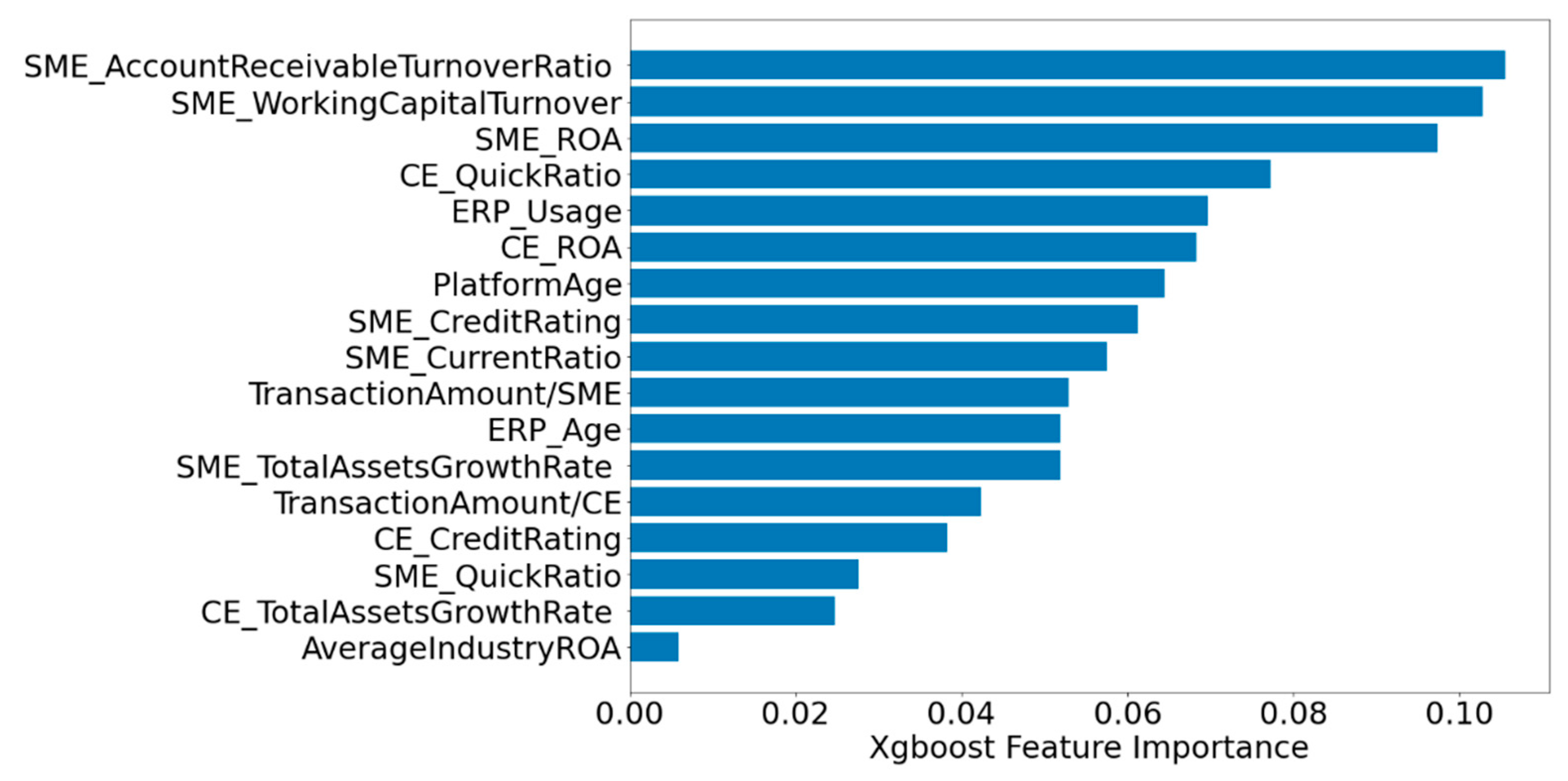
To further validate the impact of XGBoost feature selection on credit risk assessment, we first ranked the importance of all the features, and Figure 4 shows the XGBoost feature importance ranking, with the horizontal axis showing the threshold of the selected features.

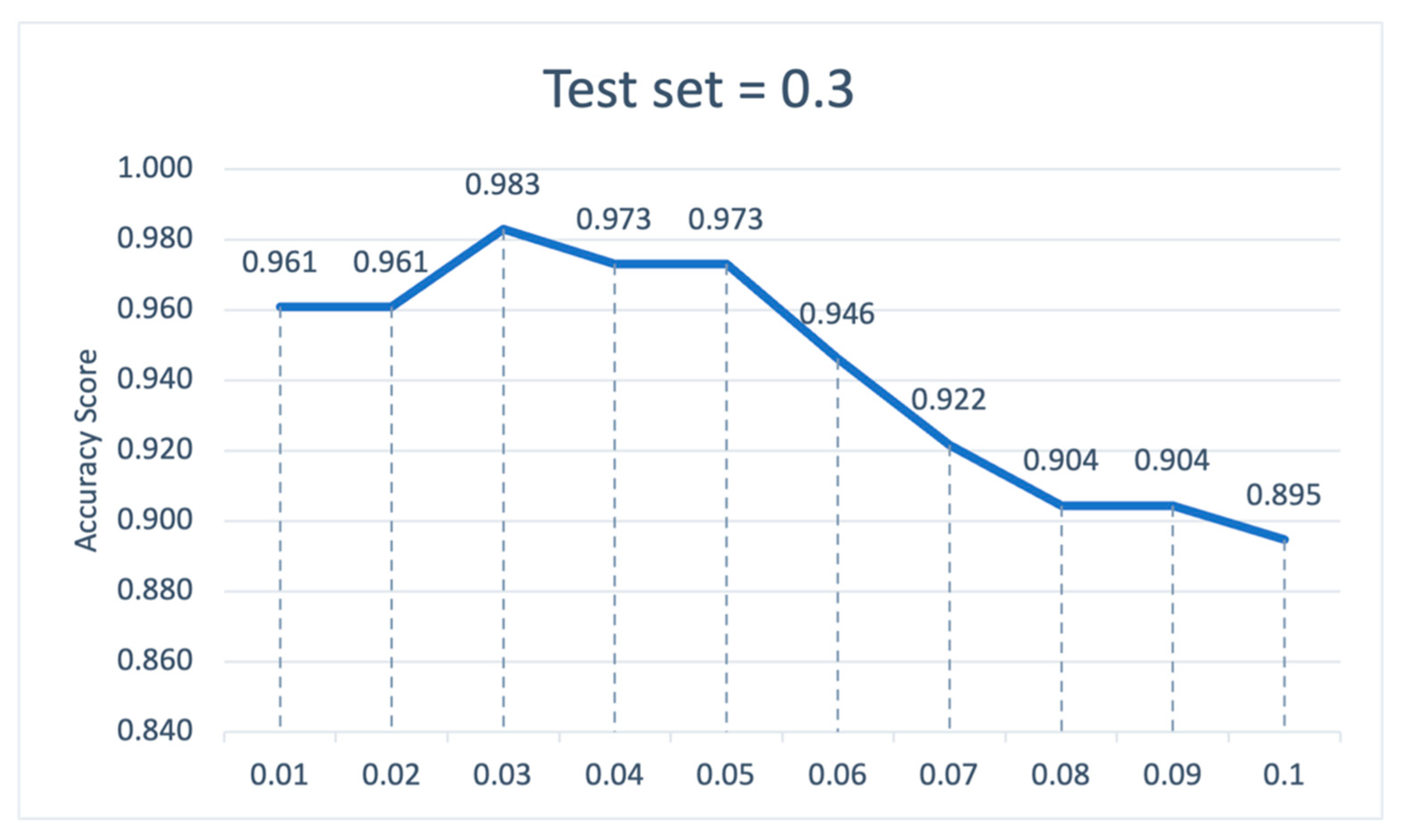
We then examine the accuracy of the assessment at different thresholds and plot the change as Figure 5. An increasing threshold means that more useless features are removed, and the accuracy of the model increases as the threshold increases until the best accuracy of the model is assessed at a threshold of 0.03 (average accuracy is 0.983), when the quick ratio of SMEs, the growth rate of total assets of the core enterprise and the average industry ROA are removed. This indicates that these three indicators are detrimental to credit risk assessment and that removing these three characteristics will result in a more accurate model. Then, as the threshold continues to increase (above 0.03), the correctness of the model starts to decline, especially when the threshold is between 0.05 and 0.08, the correctness tends to drop sharply which shows when important features are removed from the model, the correctness rate deteriorates. This indicates that feature selection has a significant impact on the effectiveness of credit risk assessment models, and that reasonable feature selection can improve model effectiveness.

5.3. The Impact of DSCF Feature

Further, for the extent to which DSCF features affect the effectiveness of credit risk assessment, we find that DSCF features occupy certain importance from the important features chart, i.e., whether the enterprise has an ERP system or not, the importance accounts for roughly 0.07 in credit risk assessment, which is an important credit risk assessment factor. The age of an enterprise’s electronic information technology platform construction, with an important share of roughly 0.065, and the year in which the ERP was used with an important share of roughly 0.055, are the more important features. In order to further confirm that the inclusion of digital supply chain financial features has an impact on the effectiveness of the credit risk assessment model, we compared the results of the XGBoost-MLP model with/without digital supply chain financial features. As shown in

Table 6. Comparison of XGBoost-MLP with/without digital SCF features.

	Average Accuracy	Recall	Precision	Type I Error	Type II Error	F-Measure	MCC
XGBoost-MLP (Threshold = 0.03) with DSCF features	0.983	0.994	0.986	0.014	0.038	0.994	0.922
XGBoost-MLP (Threshold = 0.03) without DSCF features	0.946	0.986	0.954	0.048	0.096	0.970	0.739

, the average accuracy of XGBoost-MLP without DSCF feature is 0.946, which is lower than the result of XGBoost-MLP with DSCF features, and the MCC also shows that the performance of XGBoost-MLP with DSCF features is better than when it is without DSCF features.

Moreover, this paper uses partial dependence plots (PDP) to analyze the impact of each explanatory variable in the XGBoost-MLP model on credit risk assessment (Scikit-learn in Python is used for the PDP experiment.). PDP was introduced by Friedman [79] which can be used to indicate how one of the features affects the model prediction if all other features are maintained constant. Figure 6 shows the PDP of traditional financing features of SMEs including the current ratio, working capital turnover ratio, accounts receivable turnover ratio, ROA, total asset growth rate, and the credit rating score. The vertical axis of PDP represents the probability that an SME is judged non-risky, and the horizontal axis represents the change in features. Accordingly, Figure 6 indicates that the higher the current ratio, the higher probability of non-risky SMEs, which is consistent with the result of Zhu et al. [31]. Similarly, the impact of accounts receivable turnover ratio and ROA also have a similar trend that the higher ratio, the higher probability of non-risky SMEs. The change of total asset growth rate has a slight impact on the probability though the overall impact of the total asset growth rate remains between 0.85 to 0.9. Moreover, the working capital turnover ratio has the contrary trend of probability changes that the higher the working capital turnover ratio, the lower possibility of non-risky SMEs. The highest probability of non-risky SMEs happens when the working capital ratio is below 1. Generally, the higher the accounts receivable turnover rate, the shorter the period of accounts receivable, which means that the return of funds is guaranteed and the risk of repayment is correspondingly lower. However, for working capital turnover, a high working capital turnover indicates that the company is under-capitalized and has a debt crisis. Based on the sample of the SMEs in the paper, the working capital turnover ratio of SMEs in China is generally low, and although the risk of loan repayment is low, it also indicates low capital utilization and insufficient sales. Additionally, a higher credit rating has a higher probability of non-risky SMEs and the probability increases sharply when the credit rating of SMEs is improved.

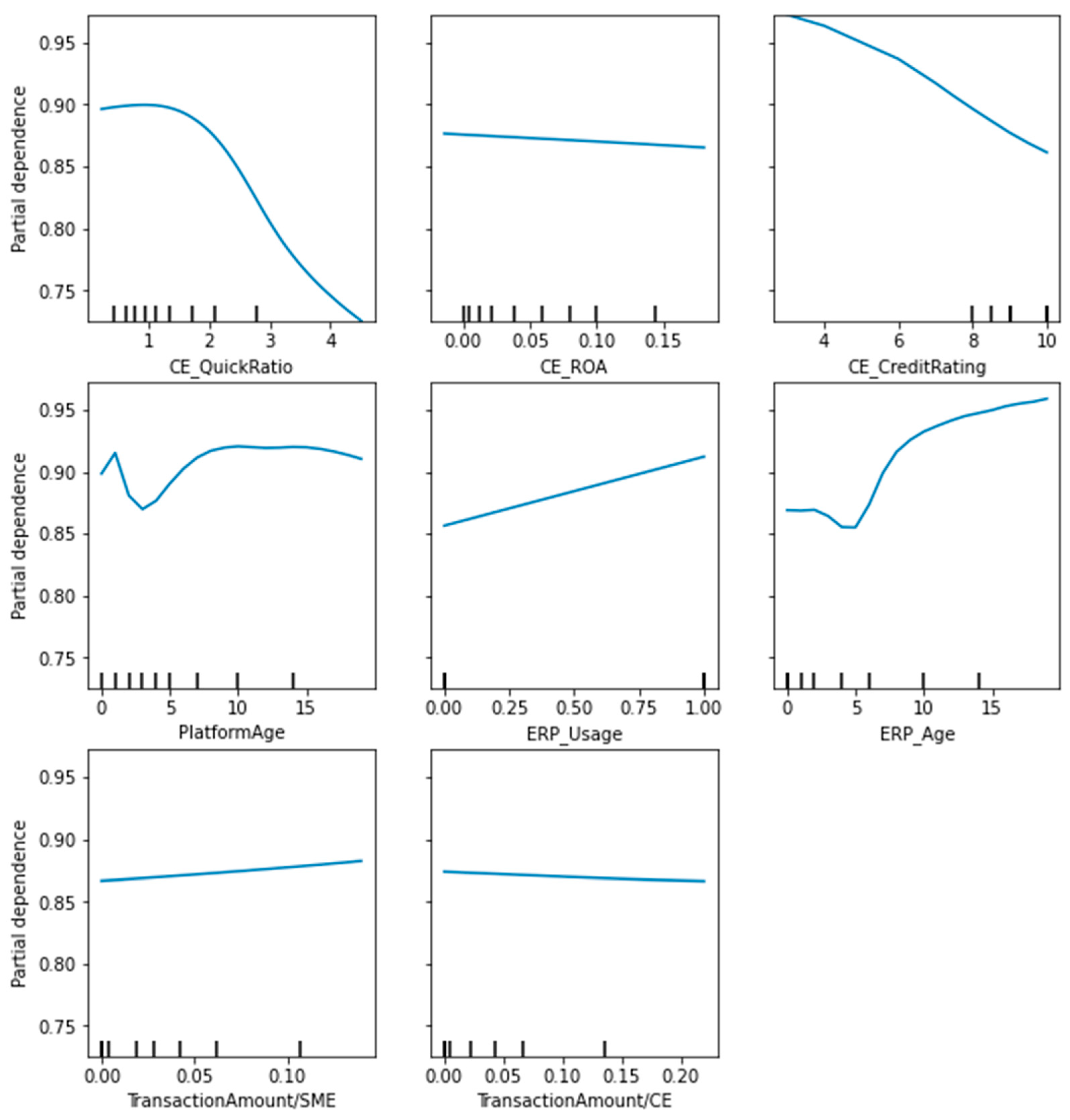
Figure 7 indicates the PDP of DSCF features of SMEs including the features of core enterprise, the digitalization feature of SMEs, and the trading features in the supply chain. There is a decreasing trend of the probability of non-risky SMEs following the increase of CE’s quick ratio, which is consistent with the result of Zhu et al. [31]. The high quick ratio of a core enterprise leads to excessive capital occupation in its quick assets, which are mostly accounts receivable in the supply chain, and this has an impact on its solvency, as there is a certain degree of uncertainty regarding the collection of accounts receivable. Therefore, for SMEs in the supply chain, a core enterprise with a high quick ratio does not enhance its own risk tolerance. It is also interesting to note that a higher return on assets (ROA) of the core firm does not improve the risk-free probability of the SME. Although a higher ROA indicates a better utilization of the assets of the core enterprise, for SMEs in the supply chain, their own repayment ability is more important. Meanwhile, we find that core enterprise with a higher credit rating does not have the higher risk-free probability of SMEs but has the opposite effect. Combined with the fact that the weight of the credit rating of core enterprises is not prominent in the feature importance ranking in Figure 4, we believe that the current source of funds for SMEs in China is complex, and SCF is not the main source of funds for SMEs, which leads to the core enterprises’ own advantage which does not effectively enhance the risk-free probability of SMEs.

Nevertheless, the DSCF features of SMEs have a more positive impact. The change in the age of platform usage is non-linear, with the lowest probability of a firm being non-risky when the age of information platform usage is around three years. Whereas, when the age of platform use is in the range of 3 to 10 years, the probability of a firm being non-risky is positively affected. Furthermore, the longer the platform is used does not increase the risk-free probability of the firm, which starts to decrease after 15 years of usage. We further use the dummy variable to describe the usage of ERP by firms, and the trend in Figure 7 shows that SMEs using ERP systems have a higher probability of being risk-free. The feature of ERP usage age is also non-linear, as the change in risk-free probability is not significant for firms with ERP usage of fewer than five years, but when firms have ERP usage of more than five years, the longer the usage time, the higher the risk-free probability. Regarding the basis of supply chain financial cooperation, the variable of the transactions between the core firm and the SME divided by SME’s sales or costs also show a positive change, with a subsequent increase in the probability of risk-free for the firm. This indicates that in the supply chain when the main business of SMEs and core enterprises has a certain regularity and a large proportion, the solvency of SMEs has certain stability and security.

6. Robustness Check

The XGBoost-MLP model achieves better credit risk assessment results than the comparison models in the designed experimental environment. In order to assess the robustness of the XGBoost-MLP model in credit risk assessment, we attempt to vary the experimental setting of the model and investigate whether changing the test set proportion in the dataset has an impact on the performance of the models. The following tables show the evaluation results for each model when the test set percentage is adjusted from 0.3 to 0.1 with the rest of the data set remaining unchanged.

Table 7. Performance of XGBoost-MLP and other machine learning methods. (Test set = 0.1).

	Average Accuracy	Recall	Precision	Type I Error	Type II Error	F-Measure	MCC
LR	0.926	0.992	0.929	0.076	0.056	0.959	0.638
KNN	0.971	0.992	0.975	0.025	0.056	0.983	0.868
NB	0.860	0.889	0.946	0.051	0.722	0.917	0.487
DT	0.956	0.966	0.983	0.017	0.222	0.974	0.818
SVM	0.971	1.000	0.967	0.034	0.000	0.983	0.867
RF	0.963	1.000	0.959	0.042	0.000	0.979	0.832
MLP	0.978	1.000	0.975	0.025	0.000	0.987	0.901
XGBoost-KNN	0.978	0.992	0.983	0.017	0.056	0.987	0.902
XGBoost-NB	0.882	0.924	0.939	0.059	0.500	0.932	0.512
XGBoost-DT	0.934	0.983	0.943	0.059	0.111	0.963	0.695
XGBoost-SVM	0.977	1.000	0.975	0.025	0.000	0.987	0.901
XGBoost-RF	0.971	1.000	0.967	0.034	0.000	0.983	0.867
XGBoost-MLP	0.978	0.989	0.986	0.014	0.077	0.987	0.901

Notes: This table presents the performance of XGBoost-MLP and other machine learning methods. All models presented in Table 7 are estimated based on the test set = 0.1. Results are estimated based on the training set of 949-observations and the test set of 408-observations from 31 March 2016–31 December 2019. LR is the logistic regression model; KNN is the k-nearest-neighbor model; NB is the naïve Bayes mode; DT is the decision tree model; SVM is the support vector machine model with radial bias function as kernel function; RF is the random forest model; MLP is the multi-layer perceptron model.

shows the performance of each model when the test set is 0.1; the average accuracy of XGBoost-MLP is the highest, and we further focus on the F-Measure which represents the harmonized average score of recall and precision. The F-Measure score of XGBoost-MLP is also the highest among the tested models. In addition, the Type I error of XGBoost-MLP is the lowest among the models, which indicates that XGBoost-MLP works best in screening for risky firms.

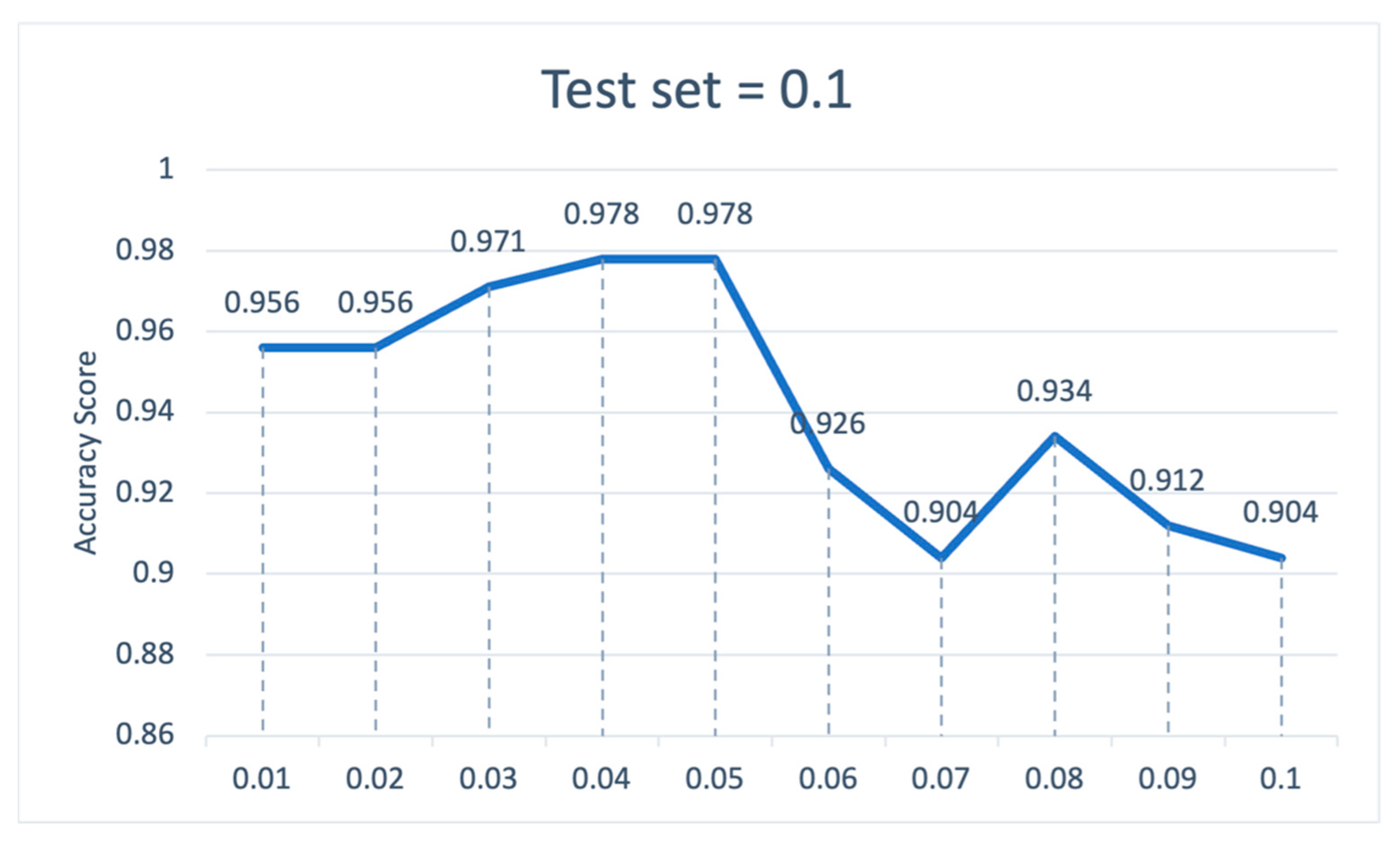
Figure 8 shows the ranking of the feature importance of XGBoost-MLP at a test set of 0.1, with the ROA of SME being the most important feature. More specifically, we find by plotting the variation in model accuracy for different thresholds (see Figure 9) that the model has the highest accuracy of 0.978 when the threshold is at 0.04 or 0.05, i.e., removing the quick ratio of SMEs, the credit rating of CE, the proportion of trading transaction on CE sales or cost, the growth rate of total assets of the core enterprise, and the average industry ROA. It is noteworthy that when the threshold rises to 0.06, the growth rate of total assets of the core enterprise and the average industry ROA is also removed, and then the accuracy of the model decreases significantly and the features removed include ERP age, usage status of ERP, the growth rate of total assets of the SME, and the credit rating of the SME.

Extra similar robustness findings supporting the main results are obtained of test set = 0.2 and 0.4, and they are available upon request. In summary, combining the different test set settings, we find that the overall model evaluation results change to some extent as the test set changes, but the average accuracy of the XGBoost-MLP is still the highest, indicating the robustness of the XGBoost-MLP model. Moreover, the most optimal test setting is when the test set is 0.3.

7. Conclusions

With the development of the industrial IoT and the digital economy, various industries and sectors will form different industrial chains and supply chains on various digital platforms in the future. DSCF is breaking the shackles of the current inertia of building digital platforms centered on finance or banks, embedding DSCF into various industrial Internet of Things and various digital economic platforms, and becoming an organic part of these digital economic platforms. In order to take DSCF as the research background, specifically from the perspective of credit risk assessment, this paper conducted research on the credit risk assessment methods of enterprises in the DSCF environment and its empirical evidence.

Firstly, the existing credit risk assessment methods in terms of their subjective and arbitrary feature selection and the poor effectiveness of linear assessment methods are analyzed in this paper. Secondly, feature importance and the role of feature selection on credit risk assessment models through XGBoost feature selection are evaluated. Then, the role of digital features for credit risk assessment in SCF is validated. We selected 1357 observations from 85 private Chinese-listed manufacturing SMEs over the period 2016–2019 to empirically test and compare the credit risk assessment models. After the feature selection by XGBoost, the five most important features were selected as accounts receivable turnover of SME, working capital turnover of SME, ROA of SME, quick ratio of CE, and ERP usage situations of SME, which improved the accuracy of risk identification by 98.3% compared to the traditional credit risk assessment models without the feature selection. The importance of the DSCF features was also verified through the XGboost feature selection. We further found that the feature selection is essential to the performance of credit risk assessment results by varying the threshold value of XGBoost feature importance ranking. The effectiveness of the risk assessment model varies depending on the threshold value set by the lending decision-maker for the feature selection process in the risk assessment, and that reasonable feature selection will improve the model effectiveness. Taking into account the various threshold values for feature selection, the accounts receivable turnover ratio of SMEs is the most important risk assessment indicator. Finally, by comparing the inclusion and removal of digital features of enterprises, we found that digital features are important for the credit risk assessment effect of digital supply chain finance, and the model with the inclusion of digital features as an assessment indicator has a higher accuracy rate, with an increase of 3.7%. This further validates that the inclusion of DSCF features in credit risk assessment is beneficial in terms of the accuracy of its risk identification.

On this aforementioned basis, this paper provides the following recommendations for the mitigation of credit risks based on DSCF. For supply chain finance platforms, including commercial banks and other financial institutions, as one of the main actors in supply chain financial services, they should be well prepared for their own risk management, credit assessment, and credit limits. Traditional credit risk assessment features such as accounts receivable turnover of SMEs, working capital turnover of SMEs, ROA of SMEs and CEs, quick ratio of CE, and credit rating of SMEs are still key characteristics for lending decision-makers. Furthermore, in the case of companies with a high degree of digitalization, such as those that actively use ERP systems or have a well-developed information technology network, the corresponding DSCF features such as the degree of ERP usage or the construction of an information technology platform should also be taken into account in the credit risk assessment. For core enterprises and SMEs, the enterprise’s accounts receivable turnover and working capital turnover are two important indicators for credit risk assessment, so enterprises are expected to be flexible in working capital and to digitize assets such as pledges to improve the speed and efficiency of circulation of the pledge. Whereas ROA, as one of the most important traditional evaluation indicators, also points out that enterprises are supposed to improve their own financial system and management system to improve their production and operation capacity. Meanwhile, the construction of digital information platforms and the usage of ERP as new indicators also provide important reference bases for credit risk assessment, and enterprises are advised to strengthen their digital development process to achieve open and transparent business data and reduce their own credit risks.

Overall, SCF is a very promising business for commercial banks, and with the continuous innovation of technology, the application of DSCF is becoming more and more widespread, and its connotations are becoming more and more enriched. Although DSCF is a future development trend and has high research value, DSCF is still in its infancy and research on it is very limited. Thus, there are some limitations in our paper. Firstly, due to the availability of data, 85 Chinese enterprises are selected as the sample for this paper. Although they are representative of the empirical samples in the context of DSCF in China, the experimental results may be biased due to the small sample. Secondly, only by comparing traditional commonly used machine learning models as a comparative analysis in this paper, we do not perform a comprehensive experimental analysis, so we will further increase the inter-model study in future research.

References

- Du, M.; Chen, Q.; Xiao, J.; Yang, H.; Ma, X. Supply Chain Finance Innovation Using Blockchain. IEEE Trans. Eng. Manag. 2020, 67, 1045–1058. [Google Scholar] [CrossRef]
- Scuotto, V.; Caputo, F.; Villasalero, M.; Del Giudice, M. A Multiple Buyer—Supplier Relationship in the Context of SMEs’ Digital Supply Chain Management. Prod. Plan. Control 2017, 28, 1378–1388. [Google Scholar] [CrossRef]
- Korpela, K.; Hallikas, J.; Dahlberg, T. Digital Supply Chain Transformation toward Blockchain Integration. In Proceedings of the 50th Hawaii International Conference on System Sciences, Hilton Waikoloa Village, HI, USA, 4–7 January 2017. [Google Scholar] [CrossRef] [Green Version]
- Banerjee, A.; Lücker, F.; Ries, J.M. An Empirical Analysis of Suppliers’ Trade-off Behaviour in Adopting Digital Supply Chain Financing Solutions. IJOPM 2021, 41, 313–335. [Google Scholar] [CrossRef]
- Ivanov, D.; Dolgui, A. A Digital Supply Chain Twin for Managing the Disruption Risks and Resilience in the Era of Industry 4.0. Prod. Plan. Control 2021, 32, 775–788. [Google Scholar] [CrossRef]
- Denison, D.G.; Holmes, C.C.; Mallick, B.K.; Smith, A.F. Bayesian Methods for Nonlinear Classification and Regression; John Wiley & Sons: Hoboken, NJ, USA, 2002; Volume 386. [Google Scholar]
- Khemakhem, S.; Boujelbene, Y. Artificial Intelligence for Credit Risk Assessment: Artificial Neural Network and Support Vector Machines. ACRN Oxf. J. Financ. Risk Perspect. 2017, 6, 1–17. [Google Scholar]
- Danenas, P.; Garsva, G. Credit Risk Evaluation Modeling Using Evolutionary Linear SVM Classifiers and Sliding Window Approach. Procedia Comput. Sci. 2012, 9, 1324–1333. [Google Scholar] [CrossRef] [Green Version]
- Bahnsen, A.C.; Gonzalez, A.M. Evolutionary Algorithms for Selecting the Architecture of a MLP Neural Network: A Credit Scoring Case. In Proceedings of the 2011 IEEE 11th International Conference on Data Mining Workshops, Vancouver, BC, Canada, 11 December 2011; pp. 725–732. [Google Scholar] [CrossRef]
- Wang, F.; Ding, L.; Yu, H.; Zhao, Y. Big Data Analytics on Enterprise Credit Risk Evaluation of E-Business Platform. Inf. Syst. E-Bus. Manag. 2020, 18, 311–350. [Google Scholar] [CrossRef]
- Timme, S.G.; Williams-Timme, C. The Financial-SCM Connection. Supply Chain. Manag. Rev. 2000, 4, 33–40. [Google Scholar]
- Berger, A.N.; Demirguc-Kunt, A.; Levine, R.; Haubrich, J.G. Bank Concentration and Competition: An Evolution in the Making. J. Money Credit Bank. 2004, 36, 433–451. [Google Scholar] [CrossRef]
- Hofmann, E. Supply Chain Finance—Some Conceptual Insights. In Logistik Management; Lasch, R., Janker, C.G., Eds.; Deutscher Universitätsverlag: Wiesbaden, Germany, 2005; pp. 203–214. [Google Scholar] [CrossRef]
- Kerle, P. Steady Supply: The Growing Role of Supply Chain Finance in Europe. Supply Chain. Eur. 2007, 16, 18. [Google Scholar]
- Camerinelli, E. Supply Chain Finance. J. Paym. Strategy Syst. 2009, 3, 114–128. [Google Scholar]
- Lyons, A.C.; Mondragon, A.E.C.; Piller, F.; Poler, R. Supply Chain Performance Measurement. In Customer-Driven Supply Chains; Springer: Berlin/Heidelberg, Germany, 2012; pp. 133–148. [Google Scholar]
- Guillén, G.; Badell, M.; Puigjaner, L. A Holistic Framework for Short-Term Supply Chain Management Integrating Production and Corporate Financial Planning. Int. J. Prod. Econ. 2007, 106, 288–306. [Google Scholar] [CrossRef]
- Gomm, M.L. Supply Chain Finance: Applying Finance Theory to Supply Chain Management to Enhance Finance in Supply Chains. Int. J. Logist. Res. Appl. 2010, 13, 133–142. [Google Scholar] [CrossRef]
- Caniato, F.; Gelsomino, L.M.; Perego, A.; Ronchi, S. Does Finance Solve the Supply Chain Financing Problem? SCM 2016, 21, 534–549. [Google Scholar] [CrossRef]
- Wuttke, D.A.; Blome, C.; Henke, M. Focusing the Financial Flow of Supply Chains: An Empirical Investigation of Financial Supply Chain Management. Int. J. Prod. Econ. 2013, 145, 773–789. [Google Scholar] [CrossRef]
- Wandfluh, M.; Hofmann, E.; Schoensleben, P. Financing Buyer–Supplier Dyads: An Empirical Analysis on Financial Collaboration in the Supply Chain. Int. J. Logist. Res. Appl. 2016, 19, 200–217. [Google Scholar] [CrossRef]
- Atkinson, W. Supply Chain Finance: The next Big Opportunity. Supply Chain Manag. Rev. 2008, 12, 57–60. [Google Scholar]
- Gobbi, G.; Sette, E. Do Firms Benefit from Concentrating Their Borrowing? Evidence from the Great Recession. Rev. Financ. 2014, 18, 527–560. [Google Scholar] [CrossRef]
- Jing, B.; Seidmann, A. Finance Sourcing in a Supply Chain. Decis. Support Syst. 2014, 58, 15–20. [Google Scholar] [CrossRef]
- Goldfarb, A.; Tucker, C. Digital Economics. J. Econ. Lit. 2019, 57, 3–43. [Google Scholar] [CrossRef] [Green Version]
- Hallikas, J.; Virolainen, V.-M.; Tuominen, M. Risk Analysis and Assessment in Network Environments: A Dyadic Case Study. Int. J. Prod. Econ. 2002, 78, 45–55. [Google Scholar] [CrossRef]
- Finch, P. Supply Chain Risk Management. Supply Chain Manag. 2004, 9, 183–196. [Google Scholar] [CrossRef]
- Yurdakul, M.; İç, Y.T. AHP Approach in the Credit Evaluation of the Manufacturing Firms in Turkey. Int. J. Prod. Econ. 2004, 88, 269–289. [Google Scholar] [CrossRef]
- Ghadge, A.; Dani, S.; Chester, M.; Kalawsky, R. A Systems Approach for Modelling Supply Chain Risks. Supply Chain Manag. 2013, 18, 523–538. [Google Scholar] [CrossRef] [Green Version]
- Zhu, Y.; Xie, C.; Wang, G.-J.; Yan, X.-G. Comparison of Individual, Ensemble and Integrated Ensemble Machine Learning Methods to Predict China’s SME Credit Risk in Supply Chain Finance. Neural Comput. Appl. 2017, 28, 41–50. [Google Scholar] [CrossRef]
- Zhu, Y.; Zhou, L.; Xie, C.; Wang, G.-J.; Nguyen, T.V. Forecasting SMEs’ Credit Risk in Supply Chain Finance with an Enhanced Hybrid Ensemble Machine Learning Approach. Int. J. Prod. Econ. 2019, 211, 22–33. [Google Scholar] [CrossRef] [Green Version]
- Orgler, Y.E. A Credit Scoring Model for Commercial Loans. J. Money Credit Bank. 1970, 2, 435. [Google Scholar] [CrossRef]
- Fitzpatrick, D.B. An Analysis of Bank Credit Card Profit. J. Bank Res. 1976, 7, 199–205. [Google Scholar]
- Lucas, A. Updating Scorecards: Removing the Mystique. In Credit Scoring and Credit Control; Thomas, L.C., Crook, J.N., Edelman, D.B., Eds.; Oxford University Press: Oxford, UK, 1992; pp. 180–197. [Google Scholar]
- Henley, W.E. Statistical Aspects of Credit Scoring; Open University: Milton Keynes, UK, 1995. [Google Scholar] [CrossRef]
- Wiginton, J.C. A Note on the Comparison of Logit and Discriminant Models of Consumer Credit Behavior. J. Financ. Quant. Anal. 1980, 15, 757. [Google Scholar] [CrossRef]
- Steenackers, A.; Goovaerts, M. A Credit Scoring Model for Personal Loans. Insur. Math. Econ. 1989, 8, 31–34. [Google Scholar] [CrossRef]
- Cramer, J.S. Scoring Bank Loans That May Go Wrong: A Case Study. Stat. Neerl. 2004, 58, 365–380. [Google Scholar] [CrossRef] [Green Version]
- Grablowsky, B.J.; Talley, W.K. Probit and Discriminant Functions for Classifying Credit Applicants-a Comparison. J. Econ. Bus. 1981, 33, 254–261. [Google Scholar]
- Makowski, P. Credit Scoring Branches Out. Credit World 1985, 75, 30–37. [Google Scholar]
- Carter, C.; Catlett, J. Assessing Credit Card Applications Using Machine Learning. IEEE Comput. Archit. Lett. 1987, 2, 71–79. [Google Scholar] [CrossRef]
- Cover, T. Estimation by the Nearest Neighbor Rule. IEEE Trans. Inf. Theory 1968, 14, 50–55. [Google Scholar] [CrossRef] [Green Version]
- Henley, W.E.; Hand, D.J. A K-Nearest-Neighbour Classifier for Assessing Consumer Credit Risk. Statistician 1996, 45, 77. [Google Scholar] [CrossRef]
- Hand, D.J. Discrimination and Classification; Wiley Series in Probability and Mathematical Statistics; Wiley: Chichester, UK, 1981. [Google Scholar]
- Pearl, J. Probabilistic Reasoning in Intelligent Systems: Networks of Plausible Inference; Morgan Kaufmann: Burlington, MA, USA, 1988. [Google Scholar]
- Hsieh, N.-C.; Hung, L.-P. A Data Driven Ensemble Classifier for Credit Scoring Analysis. Expert Syst. Appl. 2010, 37, 534–545. [Google Scholar] [CrossRef]
- Friedman, N.; Geiger, D.; Goldszmidt, M. Bayesian Network Classifiers. Mach. Learn. 1997, 29, 131–163. [Google Scholar] [CrossRef] [Green Version]
- Langley, P.; Iba, W.; Thompson, K. An Analysis of Bayesian Classi Ers. In Proceedings of the Tenth Na-Tional Conference on Articial Intelligence, San Jose, CA, USA, 12–16 July 1992; p. 15. [Google Scholar]
- Do Prado, J.W.; de Castro Alcântara, V.; de Melo Carvalho, F.; Vieira, K.C.; Machado, L.K.C.; Tonelli, D.F. Multivariate Analysis of Credit Risk and Bankruptcy Research Data: A Bibliometric Study Involving Different Knowledge Fields (1968–2014). Scientometrics 2016, 106, 1007–1029. [Google Scholar] [CrossRef]
- Odom, M.D.; Sharda, R. A Neural Network Model for Bankruptcy Prediction. In Proceedings of the 1990 IJCNN International Joint Conference on Neural Networks, San Diego, CA, USA, 17–21 June 1990; Volume 2, pp. 163–168. [Google Scholar] [CrossRef]
- Davis, R.H.; Edelman, D.B.; Gammerman, A.J. Machine-Learning Algorithms for Credit-Card Applications. IMA J. Manag. Math 1992, 4, 43–51. [Google Scholar] [CrossRef]
- Desai, V.S.; Conwayf, D.G.; Crookj, J.N.; Overstreet, G.A., Jr. Credit-Scoring Models in the Credit-Onion Environment Using Neural Networks and Genetic Algorithms. IMA J. Manag. Math. 1997, 8, 323–346. [Google Scholar] [CrossRef]
- Piramuthu, S. Financial Credit-Risk Evaluation with Neural and Neurofuzzy Systems. Eur. J. Oper. Res. 1999, 112, 310–321. [Google Scholar] [CrossRef]
- Lee, T.; Chen, I. A Two-Stage Hybrid Credit Scoring Model Using Artificial Neural Networks and Multivariate Adaptive Regression Splines. Expert Syst. Appl. 2005, 28, 743–752. [Google Scholar] [CrossRef]
- Tsai, C.-F. Financial Decision Support Using Neural Networks and Support Vector Machines. Expert Syst. 2008, 25, 380–393. [Google Scholar] [CrossRef]
- Marcano-Cedeño, A.; Marin-De-La-Barcena, A.; Jimenez-Trillo, J.; Piñuela, J.A.; Andina, D. Artificial Metaplasticity Neural Network Applied to Credit Scoring. Int. J. Neur. Syst. 2011, 21, 311–317. [Google Scholar] [CrossRef]
- Cortes, C.; Vapnik, V. Support-Vector Networks. Mach. Learn. 1995, 20, 273–297. [Google Scholar] [CrossRef]
- Stecking, R.; Schebesch, K.B. Variable Subset Selection for Credit Scoring with Support Vector Machines. In Operations Research Proceedings 2005; Haasis, H.-D., Kopfer, H., Schönberger, J., Eds.; Operations Research Proceedings; Springer: Berlin/Heidelberg, Germany, 2006; Volume 2005, pp. 251–256. [Google Scholar] [CrossRef]
- Lai, K.K.; Yu, L.; Huang, W.; Wang, S. A Novel Support Vector Machine Metamodel for Business Risk Identification. In PRICAI 2006: Trends in Artificial Intelligence; Yang, Q., Webb, G., Eds.; Hutchison, D., Kanade, T., Kittler, J., Kleinberg, J.M., Mattern, F., Mitchell, J.C., Naor, M., Nierstrasz, O., Pandu Rangan, C., Steffen, B., et al., Series Eds.; Lecture Notes in Computer Science; Springer: Berlin/Heidelberg, Germany, 2006; Volume 4099, pp. 980–984. [Google Scholar] [CrossRef]
- Schebesch, K.B.; Stecking, R. Using Multiple SVM Models for Unbalanced Credit Scoring Data Sets. In Data Analysis, Machine Learning and Applications; Springer: Berlin/Heidelberg, Germany, 2008; pp. 515–522. [Google Scholar]
- Yu, L.; Wang, S.; Lai, K.K. Developing an SVM-Based Ensemble Learning System for Customer Risk Identification Collaborating with Customer Relationship Management. Front. Comput. Sci. China 2010, 4, 196–203. [Google Scholar] [CrossRef]
- Chen, T.; Guestrin, C. XGBoost: A Scalable Tree Boosting System. In Proceedings of the 22nd ACM SIGKDD International Conference on Knowledge Discovery and Data Mining; ACM: San Francisco, CA, USA, 2016; pp. 785–794. [Google Scholar] [CrossRef] [Green Version]
- Breiman, L.; Friedman, J.H.; Olshen, R.A.; Stone, C.J. Classification and Regression Trees; Routledge: London, UK, 1984. [Google Scholar]
- Sermpinis, G.; Dunis, C.; Laws, J.; Stasinakis, C. Forecasting and Trading the EUR/USD Exchange Rate with Stochastic Neural Network Combination and Time-Varying Leverage. Decis. Support Syst. 2012, 54, 316–329. [Google Scholar] [CrossRef]
- Crook, J.N.; Edelman, D.B.; Thomas, L.C. Recent Developments in Consumer Credit Risk Assessment. Eur. J. Oper. Res. 2007, 183, 1447–1465. [Google Scholar] [CrossRef]
- Hassanniakalager, A.; Sermpinis, G.; Stasinakis, C.; Verousis, T. A Conditional Fuzzy Inference Approach in Forecasting. Eur. J. Oper. Res. 2020, 283, 196–216. [Google Scholar] [CrossRef]
- Cover, T.; Hart, P. Nearest Neighbor Pattern Classification. IEEE Trans. Inf. Theory 1967, 13, 21–27. [Google Scholar] [CrossRef]
- Sermpinis, G.; Stasinakis, C.; Hassanniakalager, A. Reverse Adaptive Krill Herd Locally Weighted Support Vector Regression for Forecasting and Trading Exchange Traded Funds. Eur. J. Oper. Res. 2017, 263, 540–558. [Google Scholar] [CrossRef] [Green Version]
- Rish, I. An Empirical Study of the Naive Bayes Classifier. In Proceedings of the IJCAI 2001 Workshop on Empirical Methods in Artificial Intelligence, Seattle, WA, USA, 4 August 2001; Volume 3, pp. 41–46. [Google Scholar]
- Antonakis, A.C.; Sfakianakis, M.E. Assessing Naive Bayes as a Method for Screening Credit Applicants. J. Appl. Stat. 2009, 36, 537–545. [Google Scholar] [CrossRef]
- Hassanniakalager, A.; Sermpinis, G.; Stasinakis, C. Trading the Foreign Exchange Market with Technical Analysis and Bayesian Statistics. J. Empir. Financ. 2021, 63, 230–251. [Google Scholar] [CrossRef]
- Quinlan, J.R. Improved Use of Continuous Attributes in C4.5. J. Artif. Intell. Res. 1996, 4, 77–90. [Google Scholar] [CrossRef] [Green Version]
- Breiman, L. Random Forests; UC Berkeley TR567; University of California: Berkeley, CA, USA, 1999. [Google Scholar]
- Cusano, C.; Ciocca, G.; Schettini, R. Image Annotation Using SVM. In Internet Imaging V, Proceedings of the ELECTRONIC IMAGING 2004, San Jose, CA, USA, 18–22 January 2004; International Society for Optics and Photonics: Bellingham, WA, USA, 2003; pp. 330–338. [Google Scholar] [CrossRef]
- Bao, W.; Lianju, N.; Yue, K. Integration of Unsupervised and Supervised Machine Learning Algorithms for Credit Risk Assessment. Expert Syst. Appl. 2019, 128, 301–315. [Google Scholar] [CrossRef]
- Stasinakis, C.; Sermpinis, G.; Psaradellis, I.; Verousis, T. Krill-Herd Support Vector Regression and Heterogeneous Autoregressive Leverage: Evidence from Forecasting and Trading Commodities. Quant. Financ. 2016, 16, 1901–1915. [Google Scholar] [CrossRef]
- Zhang, L.; Hu, H.; Zhang, D. A Credit Risk Assessment Model Based on SVM for Small and Medium Enterprises in Supply Chain Finance. Financ. Innov. 2015, 1, 14. [Google Scholar] [CrossRef] [Green Version]
- Wang, G.; Ma, J. A Hybrid Ensemble Approach for Enterprise Credit Risk Assessment Based on Support Vector Machine. Expert Syst. Appl. 2012, 39, 5325–5331. [Google Scholar] [CrossRef]
- Friedman, J.H. Greedy Function Approximation: A Gradient Boosting Machine. Ann. Stat. 2001, 45, 1189–1232. [Google Scholar] [CrossRef]
Figure 1.
Framework of digital supply chain finance.
Figure 2.
The flowchart of XGBoost-MLP.
Figure 3.
Structure of multi-layer perceptron.
Figure 4.
XGBoost feature importance ranking.
Figure 5.
The model accuracy in different threshold level.
Figure 6.
The PDP of SMEs’ traditional financing features based on the XGBoost-MLP.
Figure 7.
The PDP of DSCF features based on the XGBoost-MLP.
Figure 8.
XGBoost feature importance ranking. (Test set = 0.1).
Figure 9.
The model accuracy in different threshold levels. (Test set = 0.1).