
Projecting Mortality Rates to Extreme Old Age with the CBDX Model


1
Durham Business School, Durham University, Durham DHL 3LB, UK
2
Pensions Institute, City University of London, 106 Bunhill Row, London EC1Y 8TZ, UK
*
Author to whom correspondence should be addressed.
Forecasting 2022, 4(1), 208-218; https://0-doi-org.brum.beds.ac.uk/10.3390/forecast4010012
Submission received: 14 December 2021
/
Revised: 21 January 2022
/
Accepted: 27 January 2022
/
Published: 2 February 2022
(This article belongs to the Special Issue Mortality Modeling and Forecasting)
Abstract
:We introduce a simple extension to the CBDX model to project cohort mortality rates to extreme old age. The proposed approach fits a polynomial to a sample of age effects, uses the fitted polynomial to project the age effects to ages beyond the sample age range, then splices the sample and projected age effects, and uses the spliced age effects to obtain mortality rates for the higher ages. The proposed approach can be used to value financial instruments such as life annuities that depend on projections of extreme old age mortality rates.
Keywords:
mortality rates; Cairns–Blake–Dowd mortality model; CBDX mortality model; projection; extreme old age; life annuitiesJEL Classification:
G22; G23; J111. Introduction
The CBDX model (Dowd et al., 2020 [1]) was recently introduced as a workhorse mortality model for the adult age range (i.e., excluding the accident hump and younger ages). It applies the ‘general procedure’ (GP) of (Hunt and Blake, 2014 [2]) to identify an age-period model that fits the data well before adding in a cohort effect that captures the residual year-of-birth features arising in the original age-period model. The resulting model is intended to be suitable for a variety of populations but economises on the number of period effects in comparison with a full implementation of the GP. The CBDX model extends the Cairns–Blake–Dowd (CBD) family of mortality models (Cairns et al., 2006, 2009 [3,4]) by including an additional non-parametric age effect (or state variable (SV)) in the form of a static ‘base mortality table’.
The original CBD models were designed specifically for higher ages. As they have no age-related SVs, the models can be used to project mortality rates to any age without being constrained by the range of ages in the sample data used to calibrate the age effects. Currie (2011 [5]) shows how the original CBD models can be projected to very old ages.
Since the CBDX model has an age effect, it faces the same problem with projecting mortality at advanced ages as other models with an age effect, such as the Lee–Carter model (Lee and Carter, 1992 [6]). In this paper, we consider how the CBDX model can be used to project mortality rates beyond the upper end of the age range over which the model was estimated, allowing model users to project mortality rates out to extreme old age. This is important, for example, for a life insurer wishing to price a life annuity or sell an equity release mortgage.
The article is organised as follows: Section 2 briefly reviews the CBDX model. Section 3 illustrates our projection approach on a sample of Australian mortality data. Section 4 provides an illustrative financial application by showing how our approach can be used to price a life annuity. Section 5 looks at other approaches to projecting older age mortality rates. Section 6 concludes. Appendix A sets out the relationships between age effects, death rates, and mortality rates.
2. The CBDX Model
We begin with some definitions. First, the death rate is defined as = / where is a matrix of the number of deaths of individuals aged in year , and is the corresponding exposures matrix showing the number of individuals aged in year (or alternatively, the number of person years of aged in year ). Second, the mortality rate is defined as follows:
The CBDX model postulates that , the natural log of the death rate, is given by Equation (2):
where refers to the year of birth; , and are the age-related (i.e., base mortality table, ), period-related and cohort-related SVs, respectively; the parameters , , are fixed throughout, where and are the mean and variance of the ages in our sample age range; γ(c) is estimated as a residual and, under the null hypothesis of a good fit, we expect it to fluctuate around zero and have no trend. The difference between Equation (2) and the original CBD M7 model (Cairns et al. 2009 [4]) is that replaces , and there is now an age SV, . The version of the CBDX model we use in this article is the one in which there are three period effects (i.e., K = 3); this version is known as CBDX3.
3. Projecting Mortality to Extreme Old Age with the CBDX Model: An Empirical Example Based on Australian Data
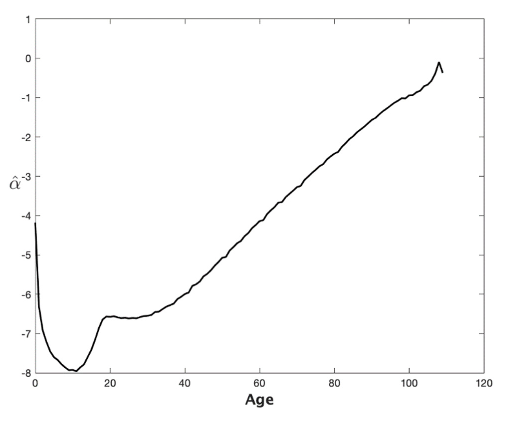
Figure 1 shows a plot of the estimated (i.e., ) for Australian males for ages varying from 0 to 109 years. In Figure 1, falls sharply after childbirth, before turning upwards in the teenage years, levelling off in the late teens and then declining again in the early years of the 20–30 age range (the ‘accident hump’); it starts to rise again in the later part of the 20–30 age range and continues rising thereafter. Of particular interest is the way in which becomes more volatile from the late 90–100 age range onwards—especially noteworthy is the hook-shaped, right-hand side tail—reflecting the estimates’ increasing sensitivity to sampling variation at higher ages.
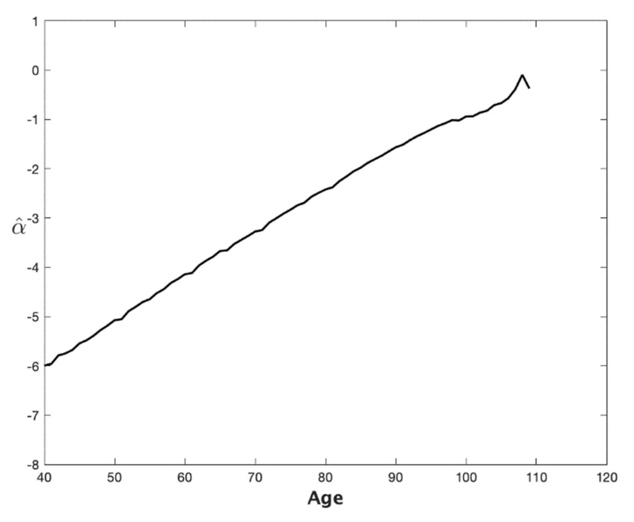
Figure 2 shows the same plot of the estimated for Australian males for ages varying from 40 to 109. Noteworthy is the near linearity of the plot up to ages in the late 90–100 age range. This near-linear fit provides the basis for the projections to higher ages. However, there is still an issue with sampling variation at very high ages, and we had to smooth out this variation. We accomplished this goal by fitting a polynomial function to the data, as explained in what follows.
We adopted the following simple approach to obtain smoothed projected (and hence ) rates extending to age 150, which we assumed to be the maximum length of life, for modelling purposes. We (a) began with a set of values of , with a sample age range, 40–95; (b) fitted a polynomial function to smooth the data over a fitted age range, 70–95; (c) used the polynomial fit to project the terms over higher ages: for illustrative purposes, we chose a projection age range of 70–150, that is, we chose to project the mortality rates of someone currently aged exactly 70 years old, who in a year’s time will be 71 if they survive, and 72 the following year, etc.; (d) spliced the fitted and projected series to produce an series spanning ages 40–150; (e) inputted this spliced series into the CBDX model (2) and then (1) to obtain a smoothed set of rates over these same ages.
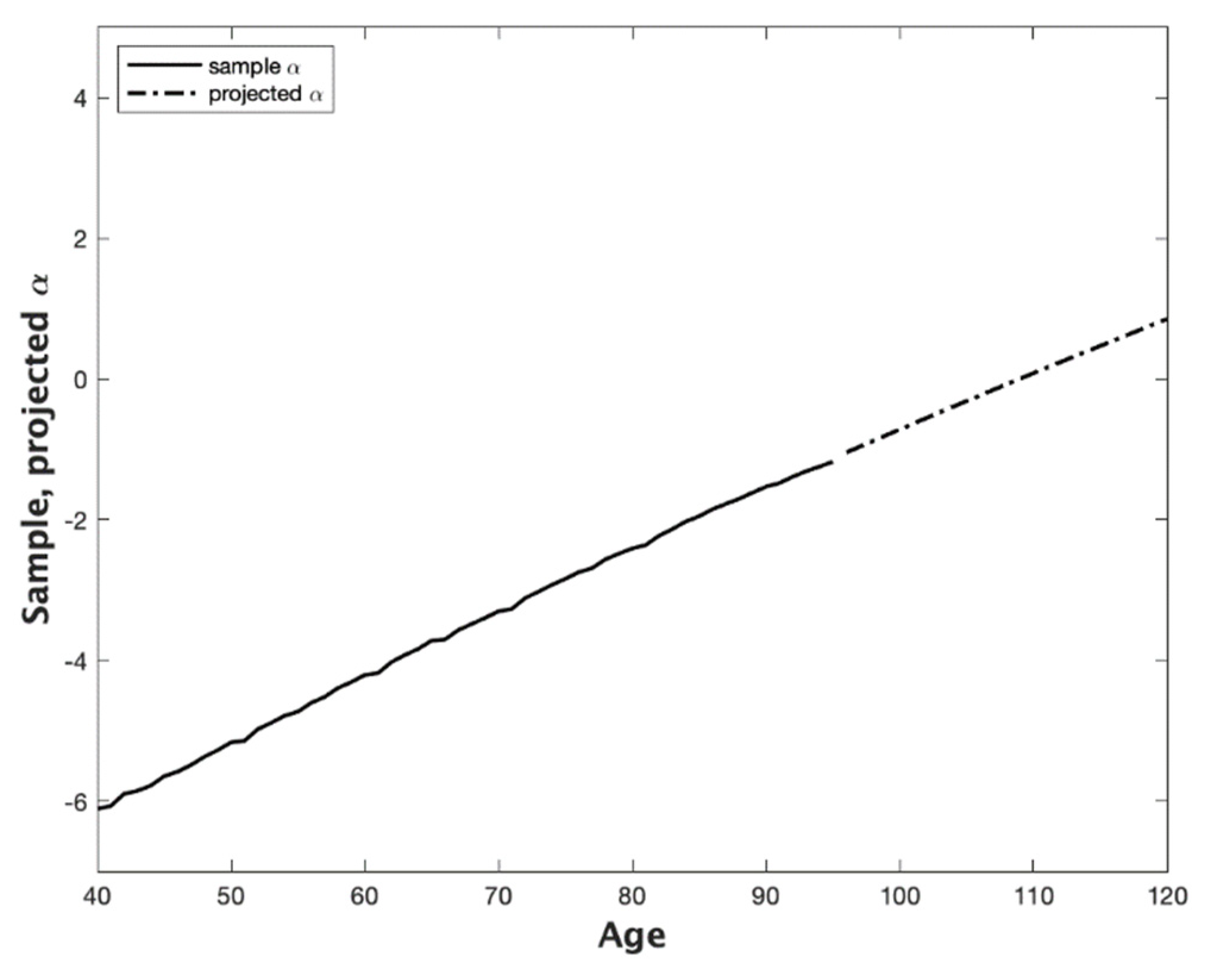
Figure 3 shows a plot (continuous line) of with ages ranging from 40 to 95 years. The dash-dotted line depicts the projections for ages 96 to 120 years (the projections extend to age 150, but Figure 3 curtails the age range at 120). This latter plot is a projection from a quadratic fit of , and we see that the projection is a well-fitted continuation of . The fitted equation is . We made the judgement that a straight line would not reflect the slight curvature shown by the plot up to the mid-years of the 90–100 age range (Figure 3) and that a cubic fit would be excessively parameterised given the slightness of that curvature. (See Lindbergson (2001 [7]) for an approach that replaces the exponential growth in a Makeham function with a straight line at very high ages). The fitted equation was obtained using the MATLAB ‘polyfit’ function. It is also worth noting that the projection is smooth and largely free of the random variation in the higher age values of .
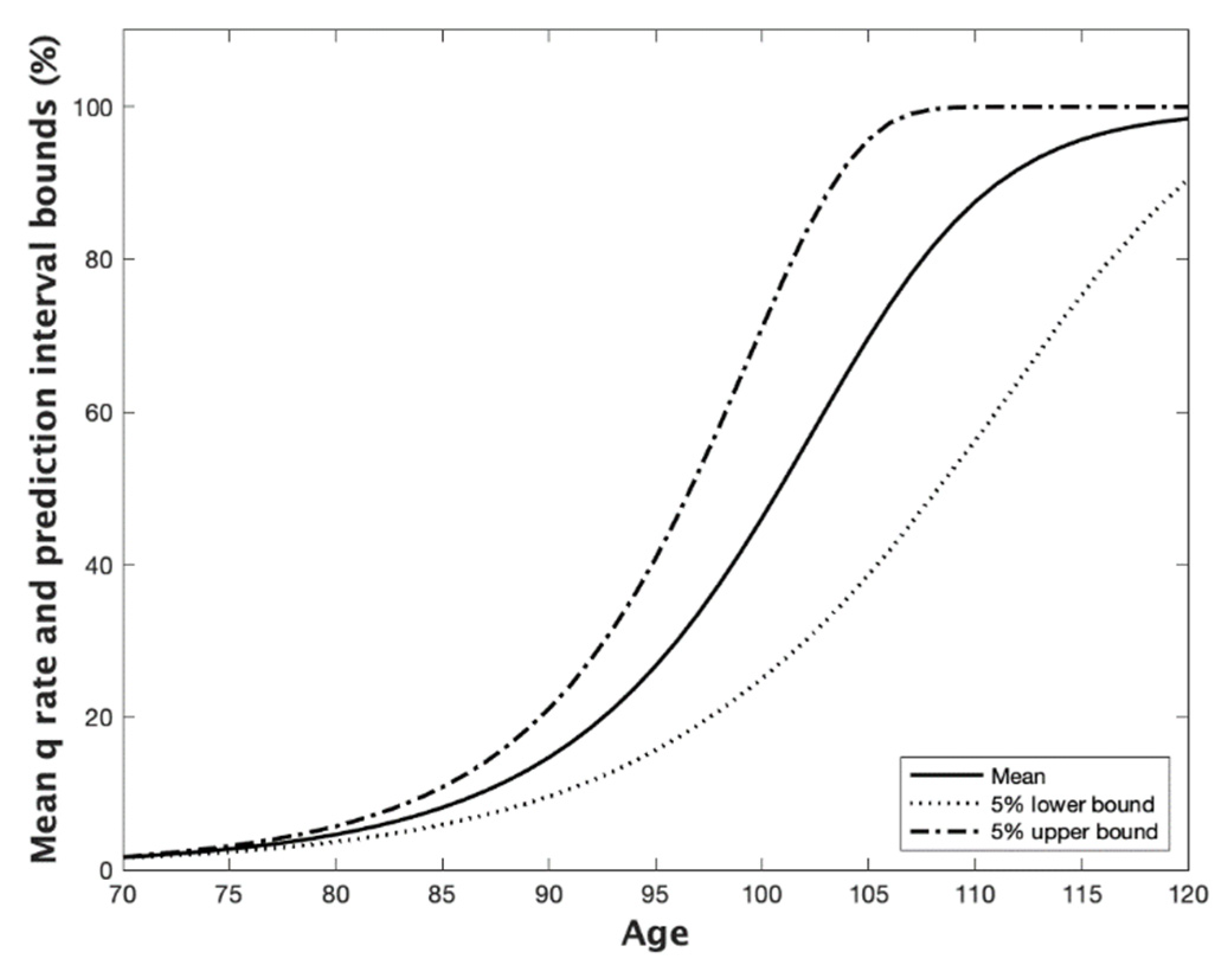
The resulting projections for the mean and 90% prediction interval for the cohort rates are shown in Figure 4, in which every member of the cohort is deemed for modelling purposes to be at their 70th birthday. The projections and their bounds rise with age and eventually converge to 100% as the age continues to rise.
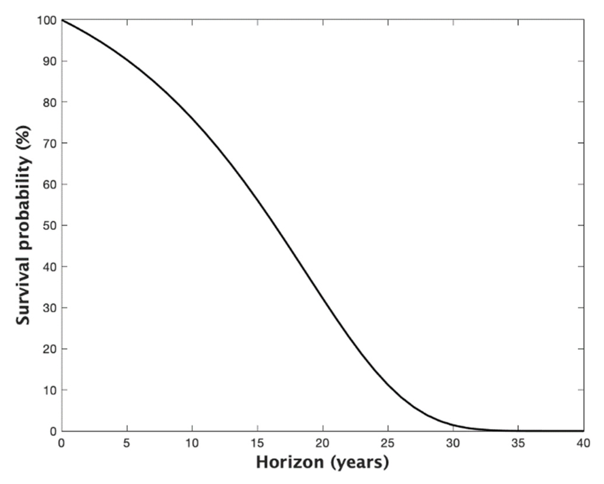
Figure 5 shows the projected survivorship probabilities corresponding to the projections in Figure 4 for an individual who just turned 70.
Table 1 shows the survival probabilities to key benchmark ages: 80, 90, 100, up to 150.
Therefore, the probability of surviving to age 100 is just over 1.4%, and the probability of surviving to age 150 is about 5.8%, with the decimal point moved 93 places to the left. To put this latter figure into perspective, the probability of surviving to age 150 is about 1/2000th of the probability of winning the national lottery 14 times in a row—possible but not too likely. (Methuselah, the grandfather of Noah, lived to the ripe old age of 969 years (See Dowd et al. 2016 [8]).
4. A Financial Application: Pricing a Life Annuity
Table 2 provides the results of a robustness exercise in which the price of a life annuity is estimated using eight different combinations of two sets of sample years (1921–2014 and 1950–2014), two sets of sample ages (40–95 and 40–80), and two sets of fitted ages (70–95 and 70–80).
The results are relatively robust: The mean annuity price is 12.80, and all prices are within the range (98.1%, 101.62%) of the mean. This suggests that the model’s mortality projections are not very sensitive to the age ranges assumed for the fitting and projection models. In principle, this is very helpful to the model user, although the findings would need to be confirmed with other datasets.
5. Other Approaches to Projecting Mortality Rates to Older Ages
It should be clear from Section 3 that smoothing and projecting mortality rates are intimately linked, since the method used for predicting often follows naturally from the method used for smoothing out the random variation in the data at high ages. Smoothing (or graduating to use the actuarial term) has a long history (see, e.g., Perks, 1932 [9]).
A number of papers (e.g., Denuit and Goderniaux, 2005 [10]; Gavrilova and Gavrilov, 2014 [11]; Gavrilov and Gavrilova, 2019 [12]) have reviewed the existing literature on smoothing and projecting future mortality rates at high ages by both demographers and actuaries.
Thatcher et al. (2002 [13]) used the ‘survivor ratio’ (SR) method, which multiplies the SR by the known number of deaths that have occurred in a given cohort, to estimate the number of survivors who are still alive. The past population can then be reconstructed by adding the estimated number of survivors to the known number of past deaths, cohort by cohort. The SR method extends the method of ‘extinct cohorts’ proposed by (Vincent 1951 [14]).
The SR method works well when mortality rates are stable but not when mortality rates are falling quite rapidly since SRs are no longer constant from one cohort to the next. Kannisto (1988, 1994, 1997 [15,16,17]) attempted to deal with this by estimating the highest age and working downwards. However, the SR estimates gradually become less and less reliable, since they become increasingly dependent on the assumptions. (They also ignore migration).
Other methods modify the so-called Gompertz law—namely, that the force of mortality exhibits exponential growth with age in the light of experience. Gavrilova and Gavrilov (2014 [11]) report that early studies (e.g., Horiuchi and Wilmoth, 1998 [18]; Thatcher et al. 1998 [19]; Thatcher, 1999 [20]) indicated that the exponential growth was followed by a period of deceleration, with slower rates of mortality increase, suggesting a logistic model might be appropriate for fitting human mortality above age 80 to account for mortality levelling off at advanced ages (Perks, 1932 [9]; Horiuchi and Wilmoth, 1998 [18]; Wilmoth et al. 2007 [21]). This mortality deceleration eventually produces ‘late-life mortality levelling-off’ and ‘late-life mortality plateaus’ at extreme old age (Gavrilov and Gavrilova, 1991 [22]).
Denuit and Goderniaux (2005 [10], DG for short) have proposed the following log-quadratic model which allows both for late-life mortality plateauing and a maximum length of life:
which is fitted to each year and high age in the dataset (DG selected an age range of 75–105), subject to the two following constraints:
- A closure constraint of for all , on the grounds that ‘even if the human life span shows no sign of approaching a fixed limit imposed by biology or other factors, it seems reasonable to retain as a working assumption that the limit age 130 will not be exceeded’ (life tables have to be closed before projection by either truncating them at a specific age (e.g., 110, 120, or 130) or the (Kannisto, 1988, 1994, 1997 [15,16,17]) method is used to close a life table, as in some European regulatory life tables; DG assumed a maximum age of 130);
- An inflexion constraint for all , which makes the rate of mortality increase with age slow down at very old ages, consistent with the early empirical demographic data.
These two constraints yield the following relationship for each
which allows to be estimated on the basis of the observations on
The completed dataset was obtained by retaining the original prior to a particular high age (DG chose 85 which is below the maximum age in their dataset), and then, the fitted values from the constrained quadratic regression were used to make projections of out to age 130.
More recent evidence indicates that mortality deceleration appears to have disappeared (Gavrilov and Gavrilova, 2019 [12]), suggesting that the inflexion constraint above may no longer be needed.
Another problem is the misreporting of the age of death of older people. Gavrilov and Gavrilova (2019 [12]) argue that age misreporting may affect the estimates of mortality at advanced ages, with even a small percentage of inaccurate data capable of distorting mortality trajectories at these ages. In most cases, age misreporting at older ages leads to mortality underestimation (Preston and Elo, 1999 [23]), and, at extreme old ages, it can lead to spurious mortality deceleration (Newman, 2018 [24]).
DG concluded that ‘no approach provides systematically satisfactory results’, while Gavrilov and Gavrilova (2019 [12]) concluded that ‘Our results demonstrate that there is no single universal answer to the question concerning the mortality pattern at extreme old ages, because this answer depends on the historical period of mortality analysis. In old historical data, late-life mortality deceleration is observed. In more recent data, mortality continues to grow exponentially with age even at very old ages. This observation may lead to more conservative estimates of future human longevity records’.
Given the problem of age-of-death errors, and since there is no theoretically ideal model for projecting mortality rates beyond the existing dataset, and since no approach currently in use provides fully satisfactory results, we decided to adopt the very simple approach outlined in Section 3—namely, using a quadratic fitting and projection model—with a very high closure constraint at age 150, but no inflexion constraint. We consider this to be at least as good as any other.
6. Conclusions
This article shows how the CBDX model can be used to project cohort mortality rates to extreme old age by fitting and projecting the age effects (or age state variables) themselves using a low-order polynomial function of age.
The proposed approach requires the application of expert judgement in a number of dimensions.
First, choosing the order of the polynomial. For the dataset we examined, plots of the age effect, , suggested that a quadratic function would suffice, while a linear function would not capture the slight curvature that was observed and a cubic fit would be over-parameterised.
Second, the following six ages should be taken into account or set:
- Age 1—minimum age of the sample age range (we chose 40);
- Age 2—maximum age of the sample age range (we chose 95);
- Age 3—minimum age of the fitted age range (we chose 70);
- Age 4—maximum age of the fitted age range (we chose 95);
- Age 5—minimum age of the projection age range, i.e., the current age of the cohort being projected (we chose 70);
- Age 6—maximum age of the projection age range, i.e., the closing age of the life table (we chose 150).
Our proposed approach produces smooth fitted mortality rates and allows modellers to project cohort mortality rates out to ages well beyond the sample age range. Our approach can also be used to price financial instruments that depend on projected cohort mortality rates that eventually increase to 1, and the most obvious example would be to price a lifetime annuity. The proposed approach is thus of considerable practical use to mortality modellers, pensions economists, and life insurers.
Author Contributions
Conceptualization, K.D. c D.B.; Methodology, K.D. and D.B.; Validation, K.D.; Visualization, K.D.; Writing— original draft preparation, K.D.; and Writing—review and editing, D.B. All authors have read and agreed to the published version of the manuscript.
Funding
This research received no external funding.
Institutional Review Board Statement
Not applicable.
Informed Consent Statement
Not applicable.
Data Availability Statement
Data were obtained from the Human Mortality Database.
Acknowledgments
The authors thank Andrew Cairns and three anonymous referees for helpful feedback. The usual caveat applies.
Conflicts of Interest
The authors declare no conflict of interest.
Appendix A. The Age State Variable, the Death Rate, and the Mortality Rate
This Appendix provides an overview of the relationships between the age state variable, the death rate, and the mortality rate.
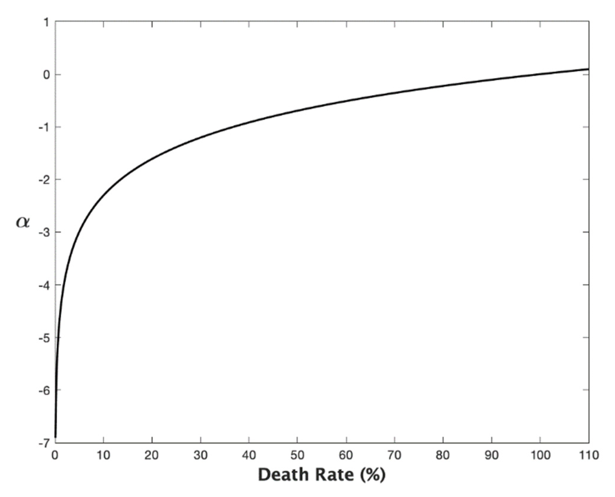
For obvious reasons, the theoretical death rate must always be bounded by 100%. However, the empirical death rate can exceed 100% because of the possibility of measurement errors in the exposures data (see, e.g., Cairns et al. 2016 [25]). Accordingly, Figure A1 allows for possible death rates in excess of 100% on the x-axis. For convenience, we now drop the ‘’ terms when they are clearly redundant. Noteworthy also is the fact that turns positive when m exceeds 100%. Thus, we should regard 100% or equivalently 0 as empirical possibilities that are associated with flawed data for extreme old age.
Figure A1.
Age effect, vs. death rate, . Notes: Based on

Since we are interested in death rates varying from 0% to 100% or slightly more, Figure A1 establishes that we should be interested in the age effect, , ranging from −7 to somewhere a little above 0.
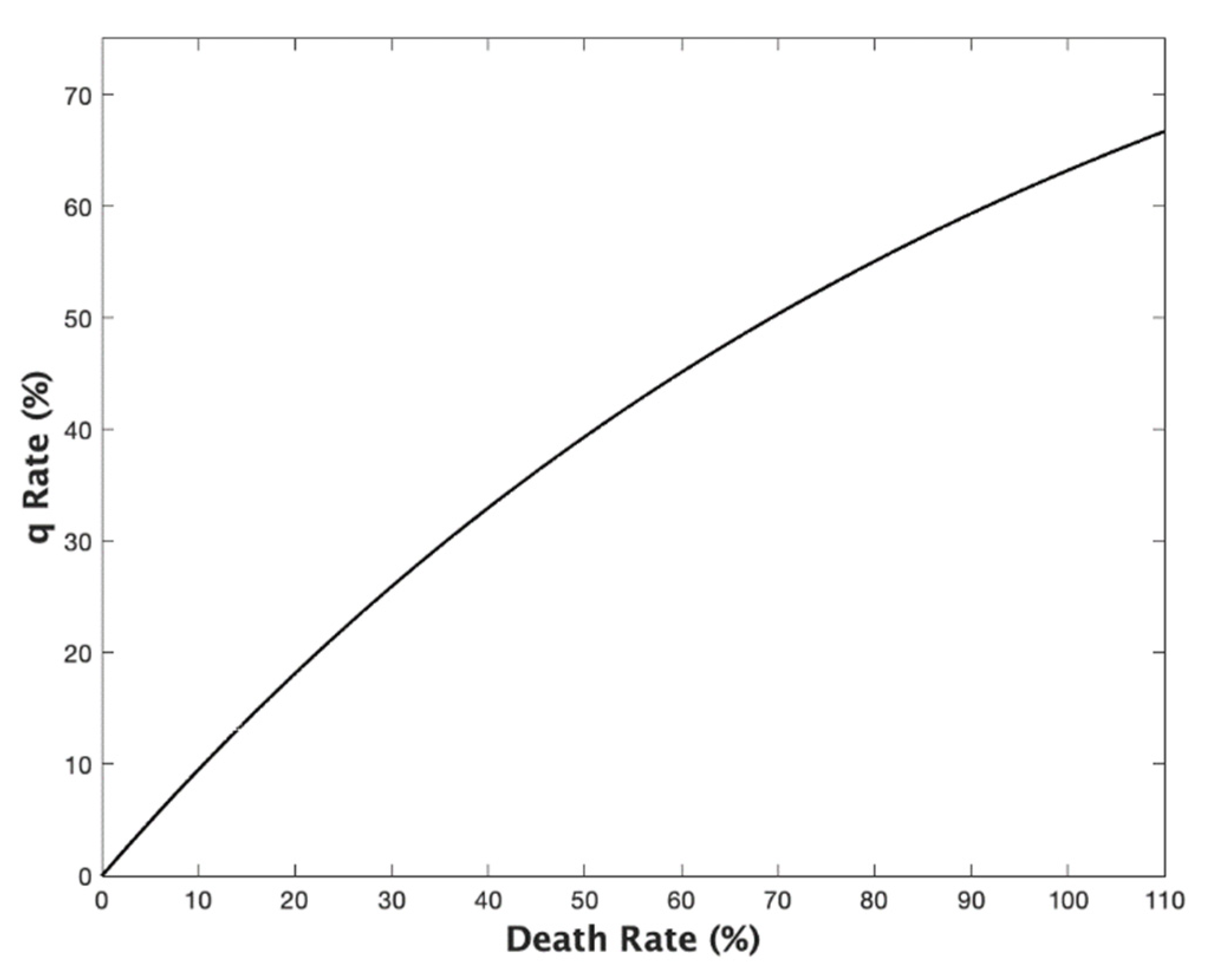
Figure A2 shows the corresponding plot of the rate vs. the rate. The concave relationship between the two rates is clearly observed. Even at an rate of 110%, which is empirically ‘off the scale’, the rate is still short of 70%.
Figure A2.
Mortality rate, vs. death rate, : I. Notes: Based on Equation (1).

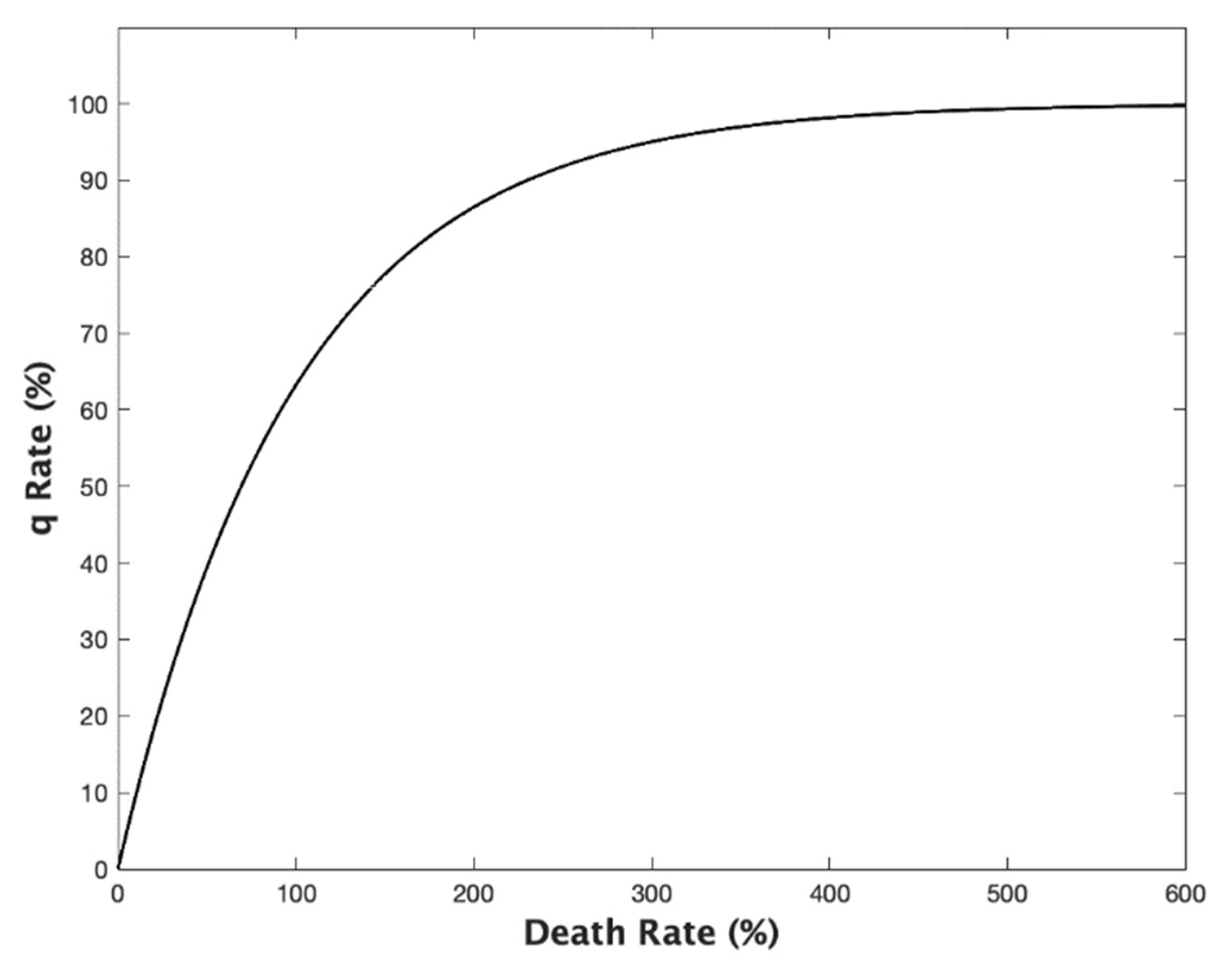
Indeed, one would have to have rates approaching 500% to obtain rates that approach 100%, as Figure A3 shows.
Figure A3.
Mortality rate, vs. death rate, : II. Notes: Based on Equation (1).

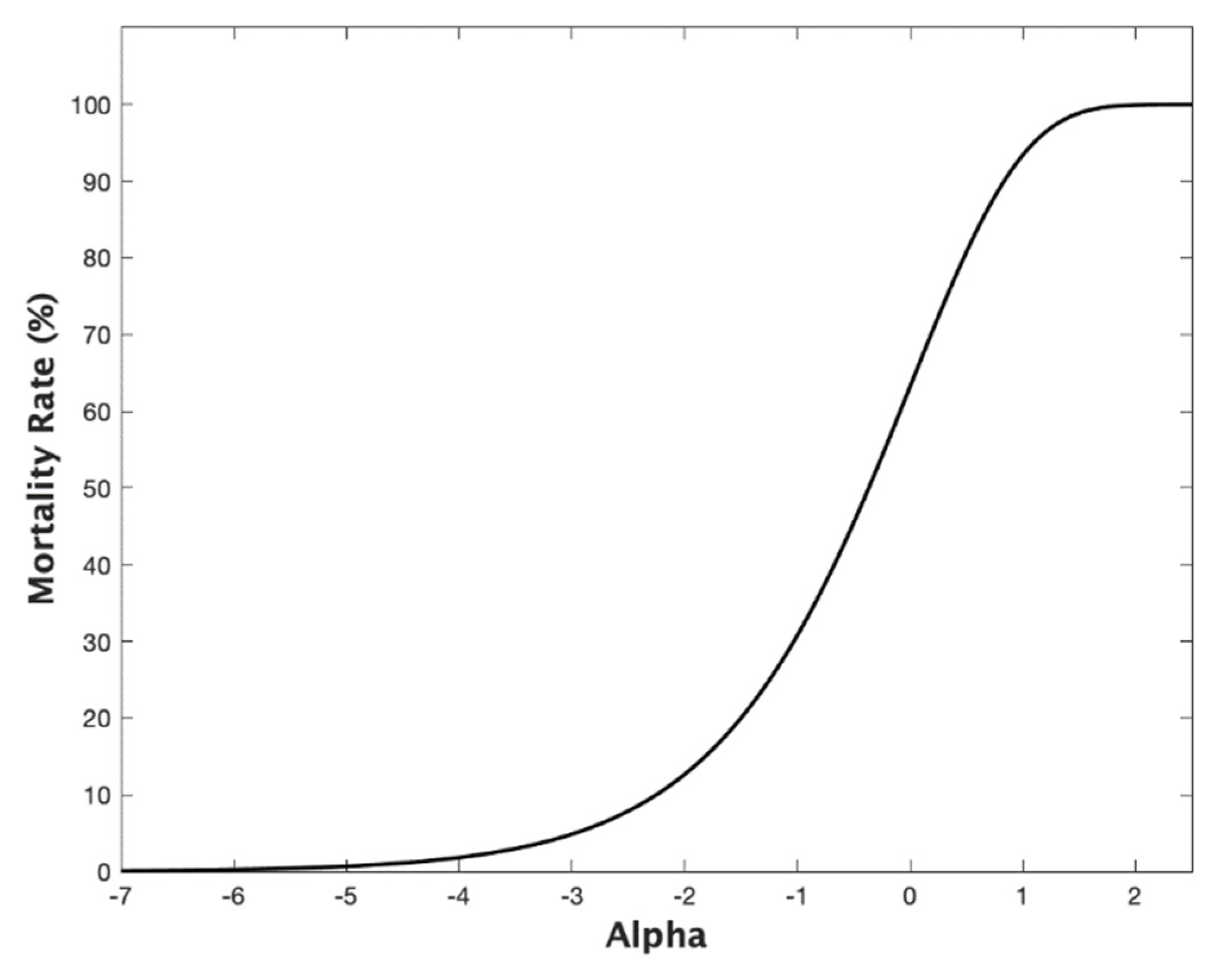
Figure A4 reports the corresponding plot of the rate vs. .
Figure A4.
Mortality rate, vs. age effect, . Notes: Based on Equation (1) and

References
- Dowd, K.; Cairns, A.J.G.; Blake, D. CBDX: A Workhorse Mortality Model from the Cairns-Blake-Dowd Family. Ann. Actuar. Sci. 2020, 14, 445–460. [Google Scholar] [CrossRef]
- Hunt, A.; Blake, D. A General Procedure for Constructing Mortality Models. N. Am. Actuar. J. 2014, 18, 116–138. [Google Scholar] [CrossRef]
- Cairns, A.J.G.; Blake, D.; Dowd, K. A Two-Factor Model for Stochastic Mortality with Parameter Uncertainty: Theory and Calibration. J. Risk Insur. 2006, 73, 687–718. [Google Scholar] [CrossRef]
- Cairns, A.J.G.; Blake, D.; Dowd, K.; Coughlan, G.D.; Epstein, D.; Ong, A.; Balevich, I. A Quantitative Comparison of Stochastic Mortality Models Using Data from England and Wales and the United States. N. Am. Actuar. J. 2009, 13, 1–35. [Google Scholar] [CrossRef]
- Currie, I.D. Modelling and Forecasting Mortality of the Very Old. ASTIN Bull. 2011, 41, 419–427. [Google Scholar]
- Lee, R.D.; Carter, L.R. Modeling and Forecasting U.S. Mortality. J. Am. Stat. Assoc. 1992, 87, 659–675. [Google Scholar] [CrossRef]
- Lindbergson, M. Mortality Among the Elderly in Sweden: 1988–1997. Scand. Actuar. J. 2001, 2001, 79–94. [Google Scholar] [CrossRef]
- Dowd, K.; Blake, D.; Cairns, A.J.G. The Myth of Methuselah and the Uncertainty of Death: The Mortality Fan Charts. Risks 2016, 4, 21. [Google Scholar] [CrossRef] [Green Version]
- Perks, W. On Some Experiments in the Graduation of Mortality Statistics. J. Inst. Actuar. 1932, 63, 12–57. [Google Scholar] [CrossRef]
- Denuit, M.; Goderniaux, A.-C. Closing and Projecting Life Tables using Loglinear Models. Bull. Swiss Assoc. Actuar. 2005, 1, 29–49. [Google Scholar]
- Gavrilova, N.S.; Gavrilov, L.A. Mortality Trajectories at Extreme Old Ages: A Comparative Study of Different Data Sources on U.S. Old-Age Mortality. Living 100 Monogr. 2014, 2014. Available online: https://www.soa.org/Library/Monographs/Life/Living-To-100/2014/mono-li14-3a-gavrilova.pdf (accessed on 20 January 2022).
- Gavrilov, L.A.; Gavrilova, N.S. New Trend in Old-Age Mortality: Gompertzialization of Mortality Trajectory. Gerontology 2019, 65, 451–457. [Google Scholar] [CrossRef] [PubMed]
- Thatcher, A.R.; Kannisto, V.; Andreev, K. The Survivor Ratio Method for Estimating Numbers at High Ages. Demogr. Res. 2002, 6, 1–18. [Google Scholar] [CrossRef]
- Vincent, P. La Mortalité des Vieillards. Population 1951, 6, 181–204. [Google Scholar] [CrossRef]
- Kannisto, V. On the Survival of Centenarians and the Span of Life. Popul. Stud. 1988, 42, 389–406. [Google Scholar] [CrossRef]
- Kannisto, V. Development of Oldest-Old Mortality, 1950–1990: Evidence from 28 Developed Countries; Odense Monographs on Population Aging No. 1; Odense University Press: Odense, Denmark, 1994. [Google Scholar]
- Kannisto, V. The Advancing Frontier of Survival; Odense Monographs on Population Aging No. 3; Odense University Press: Odense, Denmark, 1997. [Google Scholar]
- Horiuchi, S.; Wilmoth, J.R. Deceleration in the Age Pattern of Mortality at Older Ages. Demography 1998, 35, 391–412. [Google Scholar] [CrossRef] [PubMed]
- Thatcher, A.R.; Kannisto, V.; Vaupel, J.W. The Force of Mortality at Ages 80 to 120; Odense Monographs on Population Aging No. 5; Odense University Press: Odense, Denmark, 1998. [Google Scholar]
- Thatcher, A.R. The Long-term Pattern of Adult Mortality and the Highest Attained Age. J. R. Stat. Soc. Ser. A 1999, 162, 5–43. [Google Scholar] [CrossRef] [PubMed]
- Wilmoth, J.R.; Andreev, K.F.; Jdanov, D.A.; Glei, D.A. Methods Protocol for the Human Mortality Database: Version 5; Max Planck Institute for Demographic Research: Rostock, Germany, 2007. [Google Scholar]
- Gavrilov, L.A.; Gavrilova, N.S. The Biology of Life Span: A Quantitative Approach; Harwood Academic Publisher: New York, NY, USA, 1991. [Google Scholar]
- Preston, S.H.; Elo, I.T. Effects of Age Misreporting on Mortality Estimates at Older Ages. Popul. Stud. 1999, 53, 165–177. [Google Scholar] [CrossRef] [Green Version]
- Newman, S.J. Errors as a Primary Cause of Late-life Mortality Deceleration and Plateaus. PLoS Biol. 2018, 16, e2006776. [Google Scholar] [CrossRef] [PubMed] [Green Version]
- Cairns, A.J.G.; Blake, D.; Dowd, K.; Kessler, A.R. Phantoms Never Die: Living with Unreliable Population Data. J. R. Stat. Soc. Ser. A 2016, 179, 975–1005. [Google Scholar] [CrossRef] [Green Version]
Figure 1.
Australian males fitted age effect, : Ages 0 to 109. Notes: Based on the CBDX3 model applied to Australian male deaths and exposures data for sample years 1921–2014 and sample ages 0–109. Source: Human Mortality Database. All results were obtained using MATLAB.
Figure 1.
Australian males fitted age effect, : Ages 0 to 109. Notes: Based on the CBDX3 model applied to Australian male deaths and exposures data for sample years 1921–2014 and sample ages 0–109. Source: Human Mortality Database. All results were obtained using MATLAB.

Figure 2.
Australian males fitted age effect, : Ages 40 to 109. Notes: Based on the CBDX3 model applied to Australian male deaths and exposures data for sample years 1921–2014 and sample ages 40–109. Source: Human Mortality Database.
Figure 2.
Australian males fitted age effect, : Ages 40 to 109. Notes: Based on the CBDX3 model applied to Australian male deaths and exposures data for sample years 1921–2014 and sample ages 40–109. Source: Human Mortality Database.

Figure 3.
Australian males fitted age effect, , and projected age effect, : Ages 40 to 120. Notes: Based on the CBDX3 model applied to Australian male deaths and exposures data for sample years 1921–2014 and sample ages 40–95. Source: Human Mortality Database.
Figure 3.
Australian males fitted age effect, , and projected age effect, : Ages 40 to 120. Notes: Based on the CBDX3 model applied to Australian male deaths and exposures data for sample years 1921–2014 and sample ages 40–95. Source: Human Mortality Database.

Figure 4.
Projected mean and 90% prediction intervals for cohort mortality rates for Australian males just turned 70. Notes: Based on the CBDX3 model applied to Australian male deaths and exposures data for sample years 1921–2014 and sample ages 40–95. Source: Human Mortality Database. Projections make use of a spliced age effect series spanning years 70 to 120 that includes fitted for ages 70–95 and projected for ages 96–120.

Figure 5.
Survival probabilities for Australian males just turned age 70. Notes: See Figure 4 caption. For an individual aged = 70, the survival probabilities are where and .
Figure 5.
Survival probabilities for Australian males just turned age 70. Notes: See Figure 4 caption. For an individual aged = 70, the survival probabilities are where and .


Table 1.
Survival probabilities for Australian males just turned aged 70.
| Probability of survival to age 80 | 76.0% |
| Probability of survival to age 90 | 32.3% |
| Probability of survival to age 100 | 1.4% |
| Probability of survival to age110 | 1.20e−05% |
| Probability of survival to age 120 | 1.00e−18% |
| Probability of survival to age 130 | 6.30e−40% |
| Probability of survival to age 140 | 1.17e−65% |
| Probability of survival to age 150 | 5.84e−93% |
Table 2.
Life annuity prices for Australian males just turned 70.
| Sample Years | Sample Ages | Fitted Ages | Annuity Price |
|---|---|---|---|
| 1921–2014 | 40–95 | 70–95 | 12.93 |
| 1921–2014 | 40–95 | 70–80 | 12.93 |
| 1921–2014 | 40–80 | 70–95 | 11.56 |
| 1921–2014 | 40–80 | 70–80 | 11.56 |
| 1950–2014 | 40–95 | 70–95 | 13.01 |
| 1950–2014 | 40–95 | 70–80 | 13.01 |
| 1950–2014 | 40–80 | 70–95 | 12.71 |
| 1950–2014 | 40–80 | 70–90 | 12.81 |
| Mean = 12.80; Minimum = 12.56; Maximum = 13.01 | |||
Notes: Number of simulation trials = 5000; maximum possible age = 150; loading factor (to cover administration costs and provider profit) = 10%; risk-free yield curve is flat at 1%; sample years are 1921–2014 and 1950–2014; sample ages are 40–95 and 40–80; fitted ages are 70–95 and 70–80.
Publisher’s Note: MDPI stays neutral with regard to jurisdictional claims in published maps and institutional affiliations. |
© 2022 by the authors. Licensee MDPI, Basel, Switzerland. This article is an open access article distributed under the terms and conditions of the Creative Commons Attribution (CC BY) license (https://creativecommons.org/licenses/by/4.0/).
Share and Cite
MDPI and ACS Style
Dowd, K.; Blake, D. Projecting Mortality Rates to Extreme Old Age with the CBDX Model. Forecasting 2022, 4, 208-218. https://0-doi-org.brum.beds.ac.uk/10.3390/forecast4010012
AMA Style
Dowd K, Blake D. Projecting Mortality Rates to Extreme Old Age with the CBDX Model. Forecasting. 2022; 4(1):208-218. https://0-doi-org.brum.beds.ac.uk/10.3390/forecast4010012
Chicago/Turabian StyleDowd, Kevin, and David Blake. 2022. "Projecting Mortality Rates to Extreme Old Age with the CBDX Model" Forecasting 4, no. 1: 208-218. https://0-doi-org.brum.beds.ac.uk/10.3390/forecast4010012