
Switching Coefficients or Automatic Variable Selection: An Application in Forecasting Commodity Returns

1
Accounting and Finance Division, Liverpool Management School, Liverpool L69 7ZH, UK
2
Baffi CAREFIN Centre, Bocconi University, 20136 Milan, Italy
3
School of Accounting and Finance, University of Bristol, Bristol BS8 1QU, UK
*
Authors to whom correspondence should be addressed.
†
These authors contributed equally to this work.
Forecasting 2022, 4(1), 275-306; https://0-doi-org.brum.beds.ac.uk/10.3390/forecast4010016
Submission received: 30 December 2021
/
Revised: 14 February 2022
/
Accepted: 14 February 2022
/
Published: 18 February 2022
(This article belongs to the Special Issue Forecasting Commodity Markets)
Abstract
:In this paper, we conduct a thorough investigation of the predictive ability of forward and backward stepwise regressions and hidden Markov models for the futures returns of several commodities. The predictive performance relative a standard AR(1) benchmark is assessed under both statistical and economic loss functions. We find that the evidence that either stepwise regressions or hidden Markov models may outperform the benchmark under standard statistical loss functions is rather weak and limited to low-volatility regimes. However, a mean-variance investor that adopts flexible forecasting models (especially stepwise predictive regressions) when building her portfolio, achieves large benefits in terms of realized Sharpe ratios and mean-variance utility compared to an investor employing AR(1) forecasts.
1. Introduction
In the last few decades, two crucial issues have been identified by the forecasting literature applied to finance (see the recent discussion in Akyildirim et al. [1]). First, several predictors may display substantial and statistically significant predictive power, but their predictive content may be unstable over time and, as a result, it is unclear whether they can be exploited reliably (see, e.g., Rapach and Wohar [2]; Ang and Bekaert [3]; Paye and Timmermann [4]). Second, in-sample explanatory power does not necessarily translate into out-of-sample (henceforth, OOS) predictive ability, nor it ensures that the predictive relationship is stable over time (see, e.g., Welch and Goyal [5]; Campbell and Thompson [6], Clark and McCracken [7], Bossaerts and Hillion [8]).
In this paper, we tackle these two issues jointly and provide a comprehensive evaluation of the OOS predictive accuracy of two different approaches to deal with model instability and selection of relevant predictors. Namely, we compare the performance of recursively estimated stepwise regressions and hidden Markov models (HMMs, also known as Markov switching models) relative to a standard AR(1) benchmark, applied to forecasting commodity futures returns. The application of these models to the commodity space is particularly appealing. In fact, commodity prices are known to be affected by several systematic factors, ranging from macroeconomic variables capturing inflation, money supply growth, and real economic activity, to individual and aggregate commodity specific factors. However, it is unclear which of these factors, if any, may outweigh any others in forecasting commodity returns (see, e.g., Giampietro et al. [9], Guidolin and Pedio [10]) and whether the predictive relationship is stable over time or displays time-varying patterns.
There is a long-standing literature exploring the predictability of commodity returns. A first strand of literature employs traditional prediction models popular in finance (see, e.g., Bodie and Rosansky [11], Breeden [12]) or models based on commodity-specific predictors, such as hedging pressure, basis, and net trading (see e.g., Bessembinder and Chan [13], Acharya et al. [14], De Roon et al. [15], Gorton et al. [16], Gospodinov and Ng [17], Yang [18], Bakshi et al. [19]). More recently, a few attempts have been made to relate commodity returns to macroeconomic factors that are well known for explaining the cross section of bond and stock returns; see, e.g., Ahmed and Tsvetanov [20] (2016), Gargano and Timmermann [21], Kwas et al. [22], and Giampietro et al. [9]. There is also a growing literature investigating the realized volatility of commodity returns using HMMs. For instance, Luo et al. [23] recently reported that infinite HMM structures (when the infinite states parameters follow a Dirichlet process) applied to standard HAR models yield superior agricultural commodity volatility forecasts vs. standard HAR, as well as from a portfolio allocation perspective (see also Ma et al. [24]).
However, only a few papers have explored in a systematic way the predictability of commodity returns using flexible models that allow for non-linearities in the forecasting relationship when several different predictors are employed. In this respect, the paper that is closest to ours is Guidolin and Pedio [10], which uses stepwise regressions to recursively select relevant predictors in an attempt to disentangle whether commodity-specific variables improve predictive power for commodity futures returns of models otherwise based on macroeconomic factors. While exploiting a similar set of predictors, the focus of our paper is to carry out a direct comparison between variable selection and non-linear hidden Markov models where the coefficients are regime dependent. Notably, in contrast to Guidolin and Pedio [10], our paper also considers individual commodity specific factors along with aggregate ones. We are not aware of any other paper that has performed a systematic horse-race between different frameworks that allow for instability in the predictive relationship in the commodity space. However, in the presence of a multiplicity of predictors (including several macro, aggregate, and individual commodity specific factors), this seems important. Additional papers that use flexible methods to incorporate the instability in either the predictors or their coefficients include: Drachal [25], which uses Dynamic Model Averaging and Dynamic Model Selection frameworks to forecast spot oil prices; Luo et al. [23], which uses a hidden Markov HAR model to model the volatility of agricultural commodity futures; and Akyildirim et al. [1], which compares range stock return forecasts based on machine learning.
As far as our first predictive approach is concerned, we employ HMM predictive regressions in which the set of predictors that enter the model are decided ex ante by the researcher, but all the parameters of the regression are driven by a latent Markov state variable that explicitly makes the associated coefficients time-varying. The second forecasting approach relies on stepwise (either backward or forward) selection algorithms to determine which predictors (among a broad set of macro, individual, and aggregate commodity-specific factors) should be included in the forecasting model. To take into account the potentially unstable nature of the regression, we apply the selection algorithm in a recursive manner. Specifically, at all times in which a new realization of the commodity returns becomes available, this realization enters the information set and the selection procedure is performed afresh, such that a variable that belongs to the set of predictors at time t may fail to enter the model at time . Overall, the second approach privileges a careful choice of the predictive variables, which are selected using an automatic procedure that chooses the predictors that are, jointly, the most relevant from a set of candidates. In contrast, the first method focuses on the appropriate characterization of within-regime predictability at the risk of expanding the size of the models by increasing the number of coefficients. However, both approaches share an automatic nature. In fact, in HMMs, the time variation in predictive coefficients results from endogenous estimation of the Markov chain sample transitions, given a pre-specified number of hidden regimes. Similarly, in a stepwise algorithm, the rules of inclusion/exclusion of predictors are assigned given a predetermined criterion (such as information criteria, Wald test statistics, coefficient p-values, the adjusted R-square, etc.). This makes a comparison of the two modeling frameworks relevant and interesting.
There is, of course, also a growing literature on the application of HMM forecasting to a variety of other asset classes. For instance, Koki et al. [26], Koki et al. [27], and Date et al. [28] have applied a range of multi-state HMMs to the forecasting of commodity and cryptocurrency returns using predictive regressions that feature financial, economic, and cryptocurrency-specific predictors and realized volatility, similar to the approach we take. For instance, in the case of cryptocurrency returns, they report that HMMs score the highest on predictive accuracy, but also emphasize that time-varying regime switching probabilities seem to be required, even though the inferred regimes suffer from a lack of persistence. To save space and for the sake of interpretation, in our paper we have entertained only time-homogeneous HMMs. However, it is important to extend our efforts in the direction of featuring time-varying regime probabilities, which we leave to future research.
One may object that HMM models may reflect abrupt changes in the underlying hidden state and hence turn out to be more flexible than stepwise regressions. To account for the potentially time-varying nature of the regression coefficients and enhance the comparability of the stepwise and HMM frameworks, we also fit a simple regime switching AR(1) model to the VIX index and use it to classify our sample into high- and low-volatility periods. The stepwise regressions are then estimated for each of the sub-samples, and the forecasts are obtained as a probability-weighted average of the forecasts under each regime. Even though potentially effective, we acknowledge that such a hybrid model may eventually be less informative for our key research question on the comparison of HMM vs. stepwise regressions, and we would like this extension to be treated as such. Because recent literature has emphasized that the models yielding the highest statistical accuracy may fail to deliver consistent gains when the forecasts are employed in realistic economic applications (such as portfolio construction; see, e.g., Leitch and Tanner [29]; Dal Pra et al. [30]; Abhyankar et al. [31]), we evaluated the performance of the predictive models under both statistical (square and absolute value) and economic (mean-variance or MV) loss functions.
The evaluation of the alternative models was carried out OOS with reference to a January 2003–May 2018 sample (while the period from January 1989 to December 2003 was used for the initial in-sample training of the models) and for 14 monthly series of commodity futures returns (cocoa, coffee, corn, cotton, gold, orange juice, light crude oil, live cattle, platinum, sugar, silver, soy, timber, and wheat). We report three key findings. First, neither HMM nor stepwise regressions manage to systematically (or even just frequently) outperform a plain vanilla autoregressive benchmark according to statistical loss functions. In this respect, given that an AR(1) model nests a constant mean return model, we fall very close to typical literature (see the summary in Rapach and Zhou [32]) on stock return predictability, documenting that it is hard for complex statistical models to outperform even the simple historical mean predictor. Crucially, as noted by Kwas and Rubaszek [33], the random walk does not represent an appropriate benchmark when it comes to forecasting commodity returns, which display persistence and mean-revision. Therefore, we adopt an AR(1) benchmark.
Second, both stepwise and HMM regressions show stronger evidence of predictive power relative to simple benchmarks only in low-volatility regimes. At a first blush, this finding appears to be unique to the commodity space, since in the case of equities, the general result (see Rapach and Zhou [32]) is instead that asset returns become more predictable during times of market distress. However, deeper scrutiny reveals that historically, the first stage of phases of stock and bond market distress have represented low-volatility regimes for a number of commodities, especially precious metals, so the mapping is less clear-cut. In any event, when we average the predictive performances over low- vs. high-volatility regimes, we find that it remains hard for both HMM and stepwise methods to forecast well, in relative terms. Interestingly, these two results do not seem to depend on whether commodity factors are included in the analysis or not, and there is generalized, mild evidence that simpler models including only macroeconomic effects may be “rich enough” to reveal most of the predictability in the data.
Third, despite largely failing to outperform an AR(1) benchmark, complex predictive models create economic value in OOS MV portfolio tests. This is particularly evident in the case of recursively built models moving stepwise “simple to general” to avoid over-parameterizations: these turn out to dominate HMM regressions when economic metrics are taken into account. Therefore, allowing flexibility in the choice of the predictors seem to be more relevant than fully characterizing regimes when the objective is to achieve economic gains in the commodity space. These results turn out not to depend on the specific coefficient of risk aversion adopted, nor on the fact that the asset menu may also include stocks and bonds in addition to commodities. Therefore, we find evidence in the commodity space of a substantial misalignment between the typical, statistical loss functions used in applied forecasting work—under which either HMM or stepwise algorithms are of limited use—and the most common loss function in applied portfolio management work, consistent with earlier evidence in the equity space provided by Dal Pra et al. [30]. On the one hand, this illustrates that sophisticated quantitative techniques likely deserve attention in commodity forecasting. On the other hand, this stresses that the true value of such complex techniques may be revealed only by sufficiently realistic and practical relevant loss functions.
The rest of this paper is organized as follows. Section 2 describes the two methodologies used in the paper, namely, stepwise regression and HMMs. In this section, we also formally describe our backtesting framework. Section 3 describes the data. Section 4 reports detailed results on realized predictive performances under statistical loss functions. Section 5 repeats the backtesting exercise of Section 4 using economic loss functions and discusses the reasons for the strikingly heterogeneous findings. Section 6 concludes.
2. Methodology
In this paper, we assess the OOS predictive accuracy of the following (recursively estimated) predictive regressions (for , where the index refers to the different assets that we shall analyze):
where is the return between time t and t+1 of asset j, is , (for ) are principal components (PCs) selected to summarize macroeconomic information (as we shall discuss in Section 3.2), are asset-specific predictors measured for each commodity j, and are asset-specific predictors measured in aggregate across all commodities; and are dummy variables equal to one if the asset-specific factors are included in the model and equal to zero otherwise. Finally, , , and are the potentially time-varying regression coefficients. Their instability is captured alternatively by: (i) either recursively applying a stepwise (forward or backward) selection algorithm, which sets the coefficients of empirically irrelevant predictors to zero (as we shall describe in Section 2.1); or (ii) allowing the coefficients to be regime dependent under an HMM (as discussed in Section 2.2). Overall, we obtain several models:
- A simple AR(1) modelwhich represents the benchmark for our analysis and that sets the only asset-specific factor as the past performance of the asset. The standard benchmark in the forecasting literature should not be confused with our definition of the asset-specific momentum factor that also employs AR(p) models. Clearly, this model nests the standard no-change (constant mean) model often popular in empirical finance, under which the asset returns are IID. The use of the linear autoregressive models is common in the literature, see, e.g., Koki et al. [27]. Using more lag to capture stronger persistence worsened standard information criteria for the majority of the commodities examined;
- A macro factor-based HMM, where and the parameters are driven by a Markov state variable;
- A macro factor-based stepwise regression, which is obtained when and the macro variables are recursively selected by backward/forward stepwise procedures;
- An HMM model that includes macro as well as asset-specific factors, which is obtained when and the parameters (, , and ) are driven by a Markov state variable;
- An HMM model that includes macro as well as aggregate (across all commodities) asset-specific factors, obtained when and and the parameters (, , and ) are driven by a Markov state variable;
- A stepwise regression model that includes macro as well as asset-specific factors, where and the parameters are recursively selected by backward/forward stepwise procedures;
- A stepwise regression model that includes macro as well as aggregate (across all commodities) asset-specific factors, where (while ) and the variables are recursively selected by backward/forward stepwise procedures;
- A stepwise regression model that includes macro- as well as aggregate and individual asset-specific factors, which is obtained when all the dummy variables are active and the variables are recursively selected by backward/forward stepwise methods.
For the last three models, we also implement a version in which the stepwise selection applies only to macro factors, but the asset-specific factors are always included.
Our (pseudo) OOS exercise is conducted in a recursive manner (in the same spirit, for instance, as in Rapach and Zhou [32]). Monthly data spanning the period January 1989–December 2003 (for a total of 288 observations) are used to firstly estimate each of the models in consideration—both the stepwise regressions and the HMM—and produce alternative forecasts for the return of asset j over January 2004. As we proceed, new observations are added to the in-sample period in an expanding window fashion until we reach the end of the sample in May 2018. Albeit not uncommon in empirical finance, we do not entertain rolling window regressions based on a fixed number of observations because such data schemes are justified only by the presence of regimes and/or structural instability. In our application, the potential for regimes or breaks is dealt with by performing fresh stepwise model selection as the sample expands or, even more formally, by estimating HMM models. It is important to emphasize that when stepwise algorithms are used, their application is also recursive; i.e., any time that a new observation is added to the sample, the selection procedure is carried out on the extended in-sample period.
2.1. Stepwise Regressions
Consider a typical supervised learning problem at time t in which a set of inputs, , is used to forecast an outcome at time , which in our specific case is the futures return of commodity j, . A predictive regression that includes all the available N predictors is
where is a white noise disturbance with variance , is a x1 vector of predictors, and is the vector of coefficients. The best linear unbiased one-period-ahead forecast, given information up to time t, is then the linear projection
which is, however infeasible, because is unknown. Assuming that does not contain any linearly dependent predictors, can be replaced by its least squares estimate so that the resulting forecast is . Although the least squares estimate of is root-T consistent, the mean square forecast error (MSFE) increases in ; when every potential predictor in is actually not relevant, retaining the weak predictors can introduce unwarranted sampling variability to the prediction.
Among the N potential predictive variables, let us denote with the set of those that are empirically relevant (similar to Ng [34]), where is an index set containing positions in . Notably, the content of is not known to the researcher a priori and should be determined according to some criteria, e.g., on the basis of predictive accuracy. In stepwise regressions, the choice of predictive variables is carried out by an automatic procedure. In each step, a variable is considered for addition to (subtraction from) the set of forecast variables derived from an earlier iteration, on the basis of some pre-specified criterion. Under a classical stepwise regression design, there are three alternative approaches. The first is forward selection, which involves starting with no variables in the model, testing the addition of each variable using the chosen fit criterion, adding the variable (if any) whose inclusion gives the most statistically significant improvement of in-sample forecast accuracy, repeating this process until no variable improves prediction to a statistically significant extent. The second is backward elimination, which involves starting with all candidate variables, testing the deletion of each variable using a chosen model fit criterion, deleting the variable whose loss gives the most statistically insignificant deterioration of prediction accuracy (if any), and repeating this process until no further variables can be deleted without a statistically significant loss of in-sample forecasting power. The third is bi-directional elimination, a combination of the above procedures, testing at each step for variables to be included and/or excluded. In our predictive application, we pursue and compare both forward and backward designs, while we do not experiment with bi-directional elimination because its nature is complex and we know little (even less than with forward/backward elimination) from the statistics literature about its properties (A google scholar search returned only one paper with either “bidirectional stepwise” or “bi-directional stepwise” in the title, which turned out to be unrelated, and there are no papers in standard statistics or econometrics outlets with 10 or more citations).
As for the fit criteria commonly employed in stepwise regression selection, a large class of information criteria (henceforth, IC) determines the size of a model, in terms of , by finding
where is the maximum number of variables considered, is the sum of squared residuals scaled by T, and is a term that penalizes model complexity in favor of parsimony. Different choices for deliver different ICs.
In this paper, we follow Akaike [35], who has proposed to measure accuracy using the final prediction error (FPE, better known as MSFE), , which in large samples can be approximated as
minimizing FPE or as an equivalent; this reveals that the Akaike information criterion (AIC) boils down to Equation (5) with . In addition to the minimization of the FPE, the choice of can also be motivated from the perspective of minimizing the Kullback–Leibler (KL) distance. Of course, stepwise algorithms may also be implemented via sequential t- or F-testing, the latter when sets of predictors have to be jointly tested. However, sequential testing has several drawbacks. First, the size of the test represents a crucial parameter in a sequential testing procedure; if the size is too small, the critical value will be large and few variables will be selected. In addition, sequential Wald-type tests generally cannot achieve consistency in model selection procedures (as they are often based on fixed, large-sample approximations), while ICs can. Shibata [36] considers selecting the lag order of infinite order Gaussian autoregressions and assumes that the data used for estimation are independent of those used in forecasting. Using a FPE minimization loss, he shows that the (finite) p selected by the AIC is efficient in the sense that no other selection criterion achieves a smaller conditional mean squared prediction error asymptotically. Lee and Karagrigoriou [37] obtain similar results for non-Gaussian autoregressions. In fact, when it comes to consistent model selection, results tend to favor a that increases with T; Geweke and Meese [38] show in a setup with stochastic regressors that this condition is necessary for consistent model selection. For these reasons, we deem it preferable to base our selection procedure on the AIC. However, we have also obtained results for forward and backward stepwise selection based on individual Wald tests (i.e., including predictors that imply the smallest p-values from standard t-tests until these p-values are inferior to 0.10, and dropping variables that have the largest p-values until their p-values exceed 0.10). Those results are qualitatively similar to the ones described in Section 4 and remain available upon request. In preliminary tests, stepwise methods applied using the BIC criterion have led to results were indistinguishable from the AIC-based ones; therefore, they were not pursued further.
It is worth noting that stepwise regressions have been criticized in the literature because of the widespread (mal-)practice of fitting the final selected model and reporting the estimates without adjusting them to take into account the selection process (see, e.g., Butler [39] and Smith [40]), or at least appropriately adjusting the outputs related to inference and hypothesis testing (e.g., the standard errors; see Chatfield [41]). Another problem with stepwise regressions is that they search a large space of possible models and hence are prone to overfitting the data, i.e., they will often fit much better in-sample than on new, OOS data (see Smith [40]). Notably, our analysis avoids these classical problems because, rather than using stepwise regressions to perform inference, we aim to provide and test genuine OOS forecast accuracy.
2.2. Hidden Markov Models
In a hidden Markov regression model, the parameters (or a subset of them) are depend on an unobservable state variable, which we shall call . In our case, the regression in Equation (1) can be rewritten as
where the regression coefficients depend on and the rest of the terms carry the same meaning as in Equation (1). To keep things simple, we assume that is governed by a discrete, first order, ergodic, irreducible, homogeneous Markov process with a transition probability matrix , with elements
where is the probability of switching from regime j to regime i. In this paper, we consider a number of regimes K equal to two because of data limitations that we shall explain in Section 3. The vector of model parameters, , is estimated using the expectation-maximization (EM) algorithm proposed by Dempster et al. [42] and Hamilton [43], a filter that allows the iterative calculation of the one-step-ahead forecasts of the state probabilities, , given the information set , which are in turn used to construct the log-likelihood function to be maximized.
In order to guarantee a fairer comparison between HMMs and stepwise regressions, we also fit a two-state HMM on the VIX Index, which we use to separate low- and high-volatility regimes (similarly to Papanicolaou and Sircar [44]). The VIX Index is an implied volatility index computed by the Chicago Board Options Exchange (CBOE) from the price of put and call options written on the S&P 500 index; it is a market portfolio volatility proxy. The connection between the VIX and commodity returns has been established, for instance, by Kang et al. [45]:
where is and is a Markov latent state variable, as above.
Figure 1 shows the one-month ahead predicted probabilities that the VIX is in a low-volatility regime (of course, the plot for the high-volatility regime is specular, as the two predicted probabilities must sum to one by construction). The figure clearly shows that our sample may be roughly sub-divided into five sub-periods. January 1989–December 1997, January 2004–December 2007, and January 2013–May 2018 are dominated by a low mean level of the VIX, while January 1998–December 2003 and January 2008–December 2012 are clearly high-VIX sub-samples. Corresponding to each month t in our backtesting period, the forecasts from stepwise regressions are obtained by exploiting the recursively-updated predicted probabilities from the estimated HMM model in Equation (9). More specifically, two different regressions are obtained, one using only the low-volatility data as recursively classified by the HMM for the VIX, and one using the high-volatility data; then, is obtained as the weighted average between the forecasts under the high- and the low-volatility models, where the weights are the predicted regime probabilities from the model in Equation (9). In this case, we are also careful to perform forecasting endowing a user/portfolio optimizer with only the information recursively available at each point in time.
3. Data
3.1. Commodity Futures Return Series
We consider monthly return series computed from the last-trading-day-of-the-month settlement prices for 14 commodity futures contracts. The data are collected from Thomson Reuters Eikon over a January 1989–May 2018 sample. The commodities include light crude oil, seven agricultural products (cocoa, coffee, corn, cotton, sugar, soy, and wheat), three precious metals (gold, silver, and platinum), two soft commodities (orange juice and timber), and live cattle. Following a common practice in the literature (see, e.g., Gorton and Rouwenhorst [46], Basu and Miffre [47], Fuertes et al. [48]), we only focus on fully collateralized positions. This carries two implications. First, we exclude the fact that investors are allowed to operate on margin, thus using leverage. While this approach places an upper bound on the returns that an investor may achieve, it has the advantage of making investments in commodities directly comparable with the investments in other asset classes, which usually require an initial money outflow. This is, of course, crucial to our portfolio exercise. Second, by forfeiting the application of a margin system, we limit the possibility of any unintentional liquidation (due to insufficient collateral) of the position before the end of the investor’s holding period, which again makes commodity positions directly comparable to those in stocks or bonds. Because of the full-collateralization assumption, we can calculate the return on a commodity j futures position simply as
As is commonly acknowledged when it comes to using futures price data, calculating returns is made more complicated by the fact that the “front-end” contract, the one close to expiry (which is, in general, also the most liquid) has to be replaced before its natural maturity because of a need to hold the position over time (such that the delivery of the commodity is not triggered). In fact, especially in the case of commodities for which physical delivery is possible, the traders typically close their positions before the “First Notice Day”, i.e., the first day from which the exchange may impose the physical delivery of the underlying commodity, and hence before the “Last Trading Day”. To identify the First Notice Day for all contracts considered, we resort to the official trading calendar of the relevant exchange. Moreover, to try and forecast when it is most likely that traders would shift out of expiring contracts and into the second-to-expiry contract (i.e., before First Notice Day), we adopt the methodology proposed by Bakshi et al. [19]. More precisely, because an investor aims at avoiding the delivery of the commodity, we assume that she would take a position in the futures contract with the second closest maturity on the last business day of each month t, when the contract’s First Notice Day occurs.
In Table S1 in the Supplemental Material, we report the descriptive statistics for the returns on the 14 commodity futures under investigation. Interestingly, all the return series imply similar sample means and standard deviations, ranging from 0.2% per month in the case of live cattle to 0.76% in the case of light crude oil (and from 4.5% per month in the case of gold to 10.3% in the case of coffee, as far as sample standard deviations are concerned). While all series display a positive mean, a few are characterized by a negative median return (coffee, silver, and wheat), which is possible thanks to a rather large, precisely estimated positive skewness. Only live cattle and soybeans returns are characterized by negative skewness. Finally, all series display positive excess kurtosis, which, together with the widespread evidence of non-zero skewness, implies that returns are strongly non-normal.
3.2. Macroeconomic Factors
Since we aim to represent broad categories of economic activity, we consider the 132 macroeconomic and financial variables made available by Ludvigson and Ng [49], with reference to a sample starting in January 1989 and updated up to May 2018. The dataset includes several macroeconomic US variables that measure output and income, the condition of the labor market, housing, consumption, orders and inventories, and money and credit. In addition, the dataset also contains variables that summarize the conditions in the stock market (such as the log-returns of the S&¶500, the dividend yield, and the PE ratio) as well as interest and exchange rates. For the sake of brevity, we avoid listing all the variables, which are all collected from public sources. A complete list can be found in Ludvigson and Ng [49], which also details the transformations that have been applied to make the variable stationary, when appropriate. Additional information about the data and their sources are also available upon request from the authors.
In order to reduce the dimensionality of the problem, we extract principal components (PC) from this large macroeconomic dataset. It remains unfeasible or at least unpractical to let the stepwise algorithm choose among such a high number of potential predictors. In fact, when the number of candidate predictive variables, N, is large, the computational burden of the stepwise approach increases very quickly (see, e.g., Khan et al. [50]) as the enumeration of predictive regressions is necessary. When N exceeds 10, hundreds of thousands, if not millions of models must be estimated and compared to implement a stepwise approach. More precisely, we obtain the matrix of the principal components as
where is an diagonal matrix that collects the N eigenvalues of X (the matrix of the 132 predictive variables) ordered from high to low on the main diagonal, and is the orthogonal matrix spanning the column space of X.
We include in the empirical exercise only the first eight PCs and the third power of the first principal component (following Guidolin and Pedio [10]), which explain 52.2% of the variation in the sample. Interestingly, the first four PCs plus the eighth component explain 41% of the total variance of the 132 original series by themselves, confirming that there is a low-dimensional vector of shocks that drives the state of the economy. For some of the PCs, a clear economic interpretation can be inferred by looking at their loadings on the original variables. In particular, the first PC mostly reflects (i.e., it weighs heavily on) measures of employment and output (e.g., non-farm payroll employment and manufacturing output), as well as indicators of capacity utilization and new manufacturing orders. To confirm its nature as an output growth factor, the first PC shows modest correlation with prices and financial variables. The second PC reflects the dynamics of interest rate spreads, well known to be key business cycle indicators, and in fact, it is characterized by a strikingly high correlation of almost 70% with the spread between short-term Baa corporate rates and the Fed Funds Rate. The third and fourth PCs instead load heavily on the variables related to inflation and prices and, in contrast to the first PC, show modest correlations with measures of output and employment. Notably, the third PC loads heavily on consumer price indices, while the fourth loads on specific production price sub-indices. The eighth PC loads heavily on measures of aggregate stock market capitalization (whose log first differences are, of course, akin to market portfolio returns), and appears to be a sort of orthogonalized, CAPM-style factor. Unfortunately, even though they are statistically relevant and important to making the fraction of explained variance exceed 50%, the fifth, sixth, and seventh PCs fail to have a clear economic interpretation.
3.3. Commodity Factors
We compute the commodity factors using micro-level, disaggregated data provided by the US Commodity Futures Trading Commission (CFTC). In particular, the data have been extracted from the weekly “Commitment of Trader” (COT) reports, which detail for each traded futures contract the aggregate number and value of long and short positions by trader types (i.e., differentiating between “commercials”, “non-commercials”, and “non-reportables”). Such statistics are compiled at a weekly frequency on Tuesdays and published three days later, in correspondence to the market close on Friday. The CFTC classifies a trader as “commercial” when she uses futures contracts for hedging purposes as defined by Rules 1.3 (z) CFTC, 17 CFR 1.3 (z). “Non-commercials” are agents that cannot justify their trades with hedging goals, but whose nature can be clearly identified (one non exhaustive example is when these traders are financial institutions). Based on these CFTC statistics, we compute four commodity factors: the hedging pressure (HP), the basis, the momentum factor (following Daskalaki et al. [51]), and the net trading (NT) factor (as in Kang et al. [52]). Even though we follow the literature, we briefly comment on the definitions of these four factors as follows.
The HP factor (see also Basu and Miffre [47]) is measured as the difference between the negative and the positive hedging positions. More precisely, the HP for commodity j at time t is computed as the sum of the number of hedged short positions (HSP) minus the number of hedged long positions (HLP), all divided by total number of hedgers for commodity j at time t (HTP):
The basis factor is defined as the difference between the return of a portfolio of all outstanding futures on a given commodity j that shows a positive basis and a portfolio of all outstanding futures on commodity j that displays a negative basis. The basis is defined as:
where is the price of the futures contract closer to expiry and is the price of the futures contract with the next closest maturity for commodity j; the basis is positive when the futures price increases with more distant expiry dates. The NT factor for a commodity j is defined as the difference between the number of net long positions (NLP) on futures contracts at time t and the number of net long positions on the same contracts at time , divided by the total open interest (OI) on the same contracts at time t:
A high indicates that net positions are growing relative to the total number of futures contracts open for trading. Finally, time-series momentum (see, de Groot et al. [53]) is obtained by compounding the predicted returns from a family of autoregressive processes AR(p), with , estimated on each individual futures return series.
Once we have constructed the factors at the individual commodity level, we also proceed to build aggregate commodity factors. As far as the HP and NT factors are concerned, we use the formulas in Equations (12) and (14), but we apply them to all traded futures (instead of considering the futures on a specific commodity) as reported by the COT reports. As for the basis factor, we compute a simple average of the basis factors associated to each of the 14 commodities under investigation. Finally, when it comes to momentum, we compound the predicted returns from a family of AR(p) models () fitted to the simple average of the returns on the 14-commodity futures series. Whilst in the case of individual commodities, identifying momentum with a predicted return from an AR process is the only possibility we have, in the aggregate case, we may have explored building a long-short portfolio based on the lagged performance of alternative futures and commodities (e.g., going long in the five best performing commodities over the past 12 months while shorting the worst five performing commodities over the same span of time). However, to preserve consistency across alternative experiments and because the commodity-specific and aggregate commodity factors have been occasionally combined together, we have refrained from performing this robustness check.
Table S1 in the Supplemental Material shows summary statistics for the four individual commodities as well as the aggregate commodity factors. However, the interpretation of these statistics is of limited use. Means and medians of hedging pressure are structurally positive, which means that short hedged positions tend to exceed the long ones. However, most HP series display negative skewness, indicating that there are episodes/sub-periods in which long hedging positions prevail. The mean and median of the basis factors are instead predominantly negative, which indicates that typically the futures term structure is upward sloping (i.e., in contango). In this case, the prevailing positive skewness indicates that, at least episodically, commodity futures markets turn into backwardation. Finally, the net trading factor tends to display means and medians that are small and positive, an indication that trading has grown slowly relative to open interest.
4. The Statistical Predictive Performance
Table 1 reports the root MSFE (RMSFE) for a set of alternative forecasts obtained using backward or forward stepwise selection procedures in high- and low-volatility regimes defined according to the VIX Index as described in Section 2.2. The RMSFE is computed as
where j is the commodity index, refers to a specific model as defined by the selection of predictors, and 172 is the number of observations in the OOS period. Panels A to F refer to the different model specifications described in Section 2: 3 (Panel A), 6 (Panels C), 7 (Panel A), and 8 (Panel F). Panel B and D are versions of Panel C and E, respectively, where commodity specific-factors are always included, while macro factors are selected using the stepwise procedure. Panel G reports the results for the AR(1) benchmark.
Table 1 delivers only one stark result: in quiet periods (January 2004–December 2007, January 2013–May 2018), the simple AR(1) benchmark is outperformed by the stepwise predictive regressions for most commodities, while in the high-volatility regime (January 2008–December 2012), this is hardly the case. More precisely, for 11 commodities out of 14 (i.e., all excluding of live cattle, silver, and coffee), stepwise regressions forecast better than the AR(1) benchmark in the low-volatility regime; in the case of crude oil future returns, this occurs in both regimes and the RMSFE is between 6 and 7% per month vs. 8.6% in the case of an AR(1). Summing up, in 12 occasions out of 28 (as defined by the combination of the underlying commodity and the volatility regime), the framework yielding superior predictions is different from the AR(1) benchmark. Out of these 12 combinations in which stepwise predictive regressions show lower RMSFE vs. the benchmark, eight such cases involve forward, simple-to-general algorithms, which can be seen as progressive expansions of the benchmark AR(1) to improve its predictive yield. However, these empirical findings do echo the classical result in forecasting that simpler, even minimal predictive models characterized by a few parameters—or at least construction algorithms that start out with essential models and expand them on a simple-to-general path, therefore limiting model complexity in a data-driven fashion—turn out to be superior vs. more richly parameterized frameworks that, however, fit the data better. Moreover, the table shows that, while stepwise regressions are generally useful in predictive exercises in low-volatility regimes, there is no clear outperforming model in terms of which variables ought to enter the predictive regressions. However, it is worth noticing that the models where asset-specific factors are treated as fixed (i.e., they are always included) always underperform the equivalent models where the inclusion/exclusion of the factors is entirely driven by the stepwise procedure.
Table 2 compares the OOS predictive performance (as measured by the RMSFE) of stepwise predictive regressions and fully-fledged HMMs. Panels from A to C report the RMSFE for the fully-fledged HMMs, in which the coefficients of the predictive variables are allowed to change according to a first-order Markov process with two regimes. Panel A to C differ in terms of the predictive variables that are included in the model: all macro factors in Panel A; all macro and commodity-specific factors in Panel B; all macro and aggregated commodity factors in Panel C. We also experimented with a model specification where all the commodity factors (both aggregated and specific) are included in the model, but it always underperforms vs. the other HMMs and therefore, the results are omitted to save space. Panels D to I report the RMSFE for several specifications of the stepwise regressions (where commodity-specific variables are either included or excluded from the set of predictors that the stepwise algorithm is free to select, similar to Figure 1). To allow for a fair comparison, in the case of the stepwise regressions, is the weighted average of and , where the weights are the predicted regime probabilities for the model in Equation (9). Notably, the AR(1) benchmark model turns out to be hard to outperform; in fact, it represents the "winning" model (i.e., the model with the lowest RMSFE) for all but six commodities out of 14. In three of these cases, the best model is a forward stepwise regression where only macro factors are considered as potential predictors. Namely, the macro factor-based forward stepwise regressions yield an RMSFE of 8.6%, 5.2%, and 9.1% in the case of sugar, gold, and orange juice, respectively; conversely, the corresponding HMMs have an RMSFE of 10.3%, 10.9%, and 12.1%, respectively. In the case of crude oil, the lowest RMSFE is achieved by a backward stepwise regression that includes macro and commodity-specific factors (yielding a RMSFE of 7.2% vs. 8.7% of the corresponding HMM). In the remaining two cases (coffee and silver), the HMM regressions with macro and commodity-specific factors yield the lowest RMSFE (8.6% and 9.1% respectively, vs. 9.1% and 9.7% of the best stepwise regressions). Table 3 has the same structure as Table 1, but reports the mean absolute forecast error (MAFE) for each commodity j and model , computed as
Similarly to Table 1, the observations have been crudely divided into high- and low-volatility regimes according to the corresponding VIX regime. Despite the stepwise regressions outperforming the AR(1) model more frequently both in high- and low-volatility periods under an absolute value loss function rather than under a quadratic one, it is hard to identify a model specification that systematically outperforms the others. However, in six cases, a stepwise regression that selects predictors among macro factors only is the best performing model. This warns us against the temptation to include as many variables as possible in the set of candidate predictors.
Table 4 has the same structure as Table 2, but the RMSFE is replaced by the MAFE. In this case, the AR(1) benchmark is outperformed by HMM or stepwise predictive regressions in exactly a half of the cases (i.e., for seven commodities out of 14). This implies that while AR(1) tends to minimize the impact of extreme forecast errors relatively to HMM and stepwise regressions, this property is of lower relevance when the squared loss function is replaced by an absolute value one. While in the case of the RMSFE, the stepwise regressions tend to outperform the AR(1) benchmark more frequently than the HMMs, the reverse is true under an absolute value loss function. In fact, in five out of the seven cases in which the AR(1) benchmark is not the winning model, the lowest MAFE is achieved by the HMM regressions that include both macro and aggregated commodity factors. The MAFE ranges from 5.1% for soybeans to 7% for orange juice. As a matter of comparison, the best stepwise regression yields a MAFE of 6.3% in the case of soybeans and of 7.3% in the case of orange juice.
Finally, Table 5 and Table 6 provide an additional summary of the results in Table 2 and Table 4; for the cases of the quadratic (Table 5) and absolute (Table 6) loss functions, we build equally-weighted summaries of the OOS predictive performances of HMM, stepwise selection methods, and the AR(1) benchmark. The equal weighting is applied in a simple way; for each underlying commodity, we simply average the predictive performance measures across all model specifications (and backward and forward selection methods in the case of stepwise regressions). Although this choice suffers from obvious limitations, the point of these two simple tables is to tease out the ex ante expected predictive performance that would accrue to a forecaster who would not have access to any of the backtesting results in Table 1, Table 2, Table 3 and Table 4 and would randomly pick any of the models in the set, including HMM, stepwise regressions, and the benchmark. Consistent with earlier results, in both tables the “average” HMMs and stepwise regressions show considerable difficulties outperforming the benchmark. For only two commodities (corn and crude oil) out of 14 and only in the case of the MAFE, the benchmark may be outperformed by randomly picking a more complex model. This implies that even though our recursive OOS exercise has been carefully performed avoiding any hindsight bias, a forecaster that forced to pick either an HMM or a stepwise algorithm would have a very modest chance of predicting more accurately than a simple, but parsimonious AR(1) model. Interestingly, there is also some evidence that—at least for most commodities—stepwise regressions outperform HMM forecasts.
When it comes to assess the relative predictive accuracy of HMM vs. alternative prediction models, our results appear to be weaker than some recent literature concerning other asset classes; see, e.g., Catania et al. [54], Koki et al. [27], and Hotz-Behofsits et al. [55] with reference to cryptocurrencies, Luo et al. [23] and Ma et al. [24] with reference to commodity realized volatility, Guidolin and Pedio [56] with reference to risk-free interest rates, and Maruotti et al. [57] for stock returns, for which HMMs forecast very accurately both moments and densities. However, this weaker performance may also depend on the fact that, in our paper, we have entertained only time-homogeneous HMMs. In fact, using much shorter series and with a focus on energy commodities only, Date et al. [28] reported a somewhat stronger performance of HMMs.
5. Asset Allocation Performance
At a superficial level, the OOS evidence in Section 4 seems to put a final word on the issue of whether or not either automatic variable selection techniques or HMM models (or both) may deliver more accurate recursive forecasts of commodity returns vs. an off-the-shelf rudimentary AR(1) model. However, considerable literature has been accumulated on applications and theoretical reasons for why (relatively) inaccurate forecast models in a statistical perspective may turn out to yield portfolio decisions that achieve positive OOS economic value in backtesting exercises (see Leitch and Tanner [29], Abhyankar et al. [31], Dal Pra et al. [30], Gao and Nardari [58]). Of course, the reason for such findings is that when, in a recursive forecasting exercise, a given loss function is replaced by a (sufficiently different) new loss function, the OOS rankings across models may be radically affected. Therefore, in this section, we perform an additional OOS test, in the form of a recursive mean-variance (MV) asset allocation exercise that uses forecasts from the range of predictive models entertained in Section 4 to compute optimal portfolio weights and proceeds to find their implied realized performances. Such an exercise appears to be particularly sensible in light of the growing interest by investors in including commodities in their portfolios because of their diversification benefits (see, e.g., Chong and Miffre [59], Lombardi and Ravazzolo [60], Henriksen et al. [61]), although our primary goal is not to re-assess whether the inclusion of commodities in an otherwise standard portfolio generates economic value.
We use a robust MV framework that over short investment intervals is known to well approximate many other types of utility-based state preference portfolio modes. Besides the commodity future contracts already entertained above, our asset menu includes the S&P 500 (a proxy for the equity market), US 10-year treasuries, and 30-day T-bills (to proxy cash investments). We include equity, bonds, and cash on top of our 14 commodity futures for the sake of realism, to simulate the asset allocation decisions of a US investor over time. To retain symmetry and obtain a fair “playing field” across assets, we apply the same predictive models applied to commodities to stock and bond returns. For simplicity, we assume that the 1-month T-bill rate is a constant and known in advance, which we shall call .
Let be the predicted (mean) return and be the variance of asset j. An investor allocates her wealth at time t according to weights , such that the weights sum to one and that she cares (at least locally, i.e., for a one-period investment horizon) only about the conditional mean and variance of her portfolio returns, meaning that she maximizes
where represents her risk aversion coefficient. At any point in time, the portfolio conditional expected return and variance are and where is the covariance matrix of asset returns predicted at time t for time . Therefore, after substituting the constraint into the optimization, the problem in Equation (17) can be rewritten as
which leads to the solution
with .
Short sale constraints are not imposed, as most systematic traders are allowed to write futures. Following DeMiguel et al. [62], we build static one-period optimal portfolios over time, considering expanding windows of data starting from the beginning of our backtesting sample and including all data until the forecast origin. Next, we calculate the corresponding portfolio mean return, realized MV utility, and Sharpe ratio for each time t. The recursive exercise is initialized with reference to January 1989–December 2003 to produce a January 2004 portfolio and then iterated 172 times until the last estimation sample, January 1989–April 2018, to produce a portfolio for May 2018. Consistent with the literature on asset return predictability (see Bossaerts and Hillion [8]), we approximate the conditional covariance matrix with an expanding sample estimator applied to the residuals of the conditional mean equation estimates; the data are classified according to whether they are drawn from either a low- or a high-variance regime and is obtained as a weighted average of the covariance matrix in low- and high-volatility regimes, where the weights are the predicted regimes probabilities.
For the sake of robustness, we use three different values of the risk aversion coefficient (0.10, 0.25, and 0.5). To enhance the realism of the asset allocation exercise, we also consider the transaction costs implied by rebalancing the portfolio at any time t. Crucially, instead of just applying such costs on an ex post basis, we account for the fact that an investor will optimally rebalance her portfolio if and only if she can obtain an advantage in terms of an increased risk-adjusted expected return from the adjusted portfolio, i.e., when a portfolio reshuffling increases ex ante the anticipated MV utility. In our set up, this implies that she will change portfolio weights at time t only if the transaction costs of rebalancing do not exceed the portfolio expected returns at . Therefore, we also solve the portfolio problem under the following additional condition
where is a proportional transaction cost, represents a hypothetical change in weights in the case of rebalancing at time t, and represents the vector of the hypothetical weights at t in the case of rebalancing. If Equation (20) fails to hold, then an investor would not rebalance between t and , as the implied costs are higher than the resulting expected benefits, and therefore the solution to Equation (18) is , which creates an interesting path-dependent no trade region (see Mei and Nogales [63]).
As for the level of the transaction costs, we use a simplified set up in which there are only proportional transaction costs. In practice, an investor willing to re-balance her portfolio would pay two types of transaction costs: fixed costs to access the market (or infrastructure costs) and liquidity costs. Because it is difficult to make assumptions on the first type of costs, as they are likely to depend on the exact nature of an investor (e.g., whether she is an institutional investor and of what size), we do not consider them in our analysis (they are, however, likely to be negligible for a large institutional investor). In contrast, we can reasonably assume the liquidity costs to be close to the bid–ask spread as a percentage of the mid-price, therefore being proportional to the amount transacted. To estimate the parameter , we have collected daily best ask and best bid prices for commodity futures contracts for the period January 1996–December 2017. For each commodity, we estimate a daily time series for as the bid–ask spread as a percentage of the mid-price. Next, we compute the average as the grand average of all such daily values. We obtain an average value of the transaction costs across all commodities equal to approximately 0.093%. Therefore, because such estimates also vary considerably over time and across different commodities, to simplify, we set .
Table 7 and Table 8 report backtesting results for optimal asset allocation strategies without and with transaction costs, respectively. Four results emerge with strength. First, even when models cannot improve the OOS forecasting accuracy for a majority of underlying commodities, the resulting predictions may generate positive, high economic value when combined in an optimal portfolio strategy. Second, transaction costs matter, in the sense that the best performing model(s) in Table 8 sensibly differs from the one(s) in Table 7. However, in both cases, in the metrics that matter the most—i.e., realized MV utility and Sharpe ratios—it remains the case that an AR(1) model that was practically very hard to beat in Table 1, Table 2, Table 3, Table 4, Table 5 and Table 6 is regularly dominated by other models. This result admits only one exception: when transaction costs are not accounted for, the AR(1) model yields the lowest realized portfolio standard deviation; i.e., it represents the least risky forecasting strategy. Unfortunately, AR(1) also tends to return negative or very modest realized mean returns. Third, in most of the cases (with the sole exception of and in absence of transaction costs), stepwise regressions turn out to dominate fully-fledged HMM regression, irrespective of whether the Sharpe ratio or the realized utility are considered as metrics. Fourth, including commodity-specific factors (either as fixed predictors or allowing the stepwise algorithm to choose flexibly among them) turns out to often deliver the best performance both in terms of Sharpe ratio and of realized utility.
In more detail, Table 7 shows that a stepwise, forward predictive regression that includes all commodity specific factors and, if required by the recursive AIC, macro factors as well always delivers the highest realized MV objective across all choices of the risk aversion parameter. In the case of 0.1 and 0.5, this is also the case in the Sharpe ratio dimension, while for , the best performing model is obtained under an HMM when the predictors are macro-PCs and aggregated commodity factors. In general, the performance of the former model is obtained because the resulting portfolios deliver the highest realized means. This misalignment between MV and Sharpe ratio maximization is clearly possible because while, ex ante, the two-fund separation theorem guarantees that these two operations lead to identical results, on an ex post realized basis, optimizing subject to constraints that involve the riskless asset vs. will deliver different results.
For instance, when , the best stepwise regression delivers an annualized Sharpe ratio of 0.355, which outperforms the 0.245 achieved by the strongest HMM framework, while the benchmark returns a negative Sharpe ratio. Such a statistic derives from an annualized mean of approximately 4.4% and a standard deviation of 12.5%, which, of course, compares favorably with the benchmark that leads to a negative mean performance. The implied certainty equivalent return (CER)—often interpreted in the literature, see e.g., Rapach and Zhou [32], as the maximum cost that an investor would be willing to pay for switching from the benchmark to the best performing stepwise model—is massive, at 4.3% per year; the analogue CER for switching from the best performing HMM to the stepwise regression model is instead 2%. Interestingly, in Table 1, Table 2, Table 3 and Table 4, these models, and in particular the forward stepwise one, hardly ever lead to the most accurate forecasts among the available models. This represents an additional powerful warning of the fact that statistical forecasting power should not be confused with the ability to return positive economic value.
Tables S2–S6 (panels A of each) in the Supplementary Material, show that the best performing model in Table 7 is on average mostly invested (between 80 and 85%) in US 10-year Treasury Notes, while the stock market weight is on average negative, although it hides considerable variation. Of course, this is relatively unsurprising, as between 2004 and 2018, government bonds have yielded very high average excess returns, both because long-term rates have dropped to levels below 3% on several occasions and because short-term rates have been practically zero between 2009 and 2015. The position in commodity futures is therefore long in net terms on average, in the order of 14–18% of the total, but with a few notable short positions (silver, soybeans, wheat) that go to finance even larger long positions, occasionally exceeding 5% of the total (corn, gold, live cattle), which is rather massive in relative terms.
Table 8 reports results structured in the same way as in Table 7, when sensible transaction costs are imposed. Interestingly, the simple two-parameter AR(1) benchmark loses any specialty and three models emerge to our attention. On the one hand, across all values for , a forward stepwise algorithm based on macro-PCs and individual commodity-specific factors always returns the lowest realized portfolio volatility. On the other hand, for and 0.25, the model generating the top realized Sharpe ratio and MV utility is a stepwise forward regression that includes the macro-PCs and aggregate commodity factors when the latter are always included. For instance, when , this model delivers an annualized Sharpe ratio of 0.665, which outperforms the 0.336 yielded by the best HMM, while the benchmark AR(1) returns a Sharpe ratio of 0.296. Such a statistic derives from an annualized mean of 7.8% and a standard deviation of 11.7%; the implied CER of switching from the benchmark to the best performing stepwise model is another massive 6.2% per year; the analogue CER for switching from the best performing HMM to the stepwise regression model is an equally sizeable 4.4%. Besides, we note that when compared to Table 7, in Table 8 most statistics concerning the realized performances increase; this is a result of the fact that transaction costs are applied on an ex ante basis and therefore, they prevent the implementation of portfolio strategies that would fail to be value-enhancing. Tables S2 through S6 in the Supplementary Material (panels B of each) show that when transaction costs are brought into the picture, the resulting optimal asset allocations turn less extreme, in the sense that the demand for long-term government bonds declines to between 70 and 85%, while a positive weight for equities appears. As far as commodity futures are concerned, transaction costs reduce the average commitment to many commodities and, at least in the case of forward stepwise forecasts, one finds evidence of an interesting strategy of long gold and short platinum).
Finally, a comparison between Figure 2 and Figure 3 shows how the winning model from Table 8 (a forward stepwise regression model with macro and aggregate commodity factors included) displays timing ability for commodity returns (see Figure 3) because commodity weights spike before and during a few well-known commodity bull market periods. In contrast, when a simple AR(1) model is used to predict future returns, the asset allocation is overwhelmingly tilted towards 10-year Treasury bonds (as depicted in Figure 2) without much timing occurring, either for good or for bad.
6. Conclusions
We have performed a systematic OOS comparison of the performance of two general sets of forecasting methods, i.e., hidden Markov models (also known as Markov switching models) vs. the often-neglected stepwise predictive regressions, with reference to an important application in commodity futures returns. Loosely speaking, both HMM and stepwise methods represent variable selection techniques, even though HMM simply allows coefficients to take different values (zero included) in different regimes. Both forecasting approaches are combined with dimension reduction techniques used to summarize the information content of as many as 132 macroeconomic variables in a much smaller set of representative principal component factors. These macro factors are supplemented with a standard set of commodity factors (hedging pressure, basis, net trading, and momentum) implemented in two ways: at the aggregated level and at the individual commodity level.
Our OOS backtesting effort is systematic and conducted under four alternative loss functions. The first two functions are typical of the statistical forecasting literature and consist of the squared and the absolute value losses, implying that RMSFE and MAFE are used as summaries, respectively. The remaining two loss functions are the realized portfolio Sharpe ratio and MV utility, when the portfolio is built upon optimal weights computed solving a standard MV portfolio problem. Although the two loss functions are well understood, they are value functions of the underlying optimization problem and, as such, they are not only of a more applied, practical nature, but are also more complex.
Our key finding is striking: while neither HMM nor stepwise regressions manage to systematically (or even frequently) outperform a plain vanilla AR benchmark according to RMSFE or MAFE statistical loss functions, they create economic value in OOS MV portfolio tests, particularly in the case of stepwise regressions. Interestingly, because we impose transaction costs not only ex post, but also ex ante, meaning that an investor will use the forecasts of a model only when they increase expected utility, the improvement from using the forecasts from our flexible models reaches its maximum under plausible and proportional transaction costs.
A number of extensions are possible. First, we have not dealt with the performance of regularization methods (such as ridge regressions or, more generally, least absolute shrinkage selection operators (LASSO)). On the one hand, as discussed by Ng [34], the opposition between stepwise regressions based on information criteria and regularization methods is illusory, as all general cases relate to their own special cases; stepwise regressions based on information criteria are indeed cases of norm regularization methods (i.e., the shrinkage does not depend on the estimated regression coefficients, but only on their number). Moreover, work by Efron et al. [64] on least angle regressions (LAR, which is a generalization of LASSO) presents LASSO as a forward stage-wise regression. On the other hand, LASSO methods have witnessed an increasing trend and their exploration seems to be justified. Second, we have not experimented with other methods to deal with the instability in predictive regressions such as forecast combinations (see, e.g., Rapach et al. [65] and Caldeira et al. [66]) or Bayesian model averaging (see, e.g., Dangl and Halling [67], Johnson and Sakoulis [68]), which we shall leave for future research. Third, the literature has explored the integration of the steps of dimension reduction and of variable selection by optimizing composite objective functions, obtaining interesting payoffs in prediction exercises even under non-high dimensional settings (see, e.g., Lansang and Barrios [69]). Fourth, on methodological grounds, we have kept the complexity of our application of HMMs to a minimum by working with two-state models, but concurrent work (also applied to other asset classes; see e.g., Catania et al. [54], Koki et al. [27], Hotz-Behofsits et al. [55]) has shown the advantages of flexible Bayesian MCMC estimation approaches in terms of resulting density forecast accuracy. Akyildirim et al. [1] is a recent example of a comparison of range-forecasting techniques to asset (in this case, stock) returns inspired by modern applications of machine learning, which shows that our study might be fruitfully extended to compare the forecasting power of HMM and automatic model selection techniques with machine learning algorithms. Of course, it would be interesting to check whether such an integration may lead to forecast improvements in our application.
Supplementary Materials
The following supporting information can be downloaded at: https://0-www-mdpi-com.brum.beds.ac.uk/article/10.3390/forecast4010016/s1, Table S1: Descriptive statistics for commodity futures returns and the factors; Table S2: Optimal Asset Allocation–Hidden Markov Models; Table S3: Optimal Asset Allocation–Stepwise Regression Models Based on Macro Principal Components Only; Table S4: Optimal Asset Allocation–Stepwise Regression Models Based on Macro Principal Components + Commodity-Specific Factors (Always Included); Table S5: Optimal Asset Allocation–Stepwise Regression Models Based on Macro Principal Components + Commodity-Specific Factors; Table S6: Optimal Asset Allocation–Stepwise Regression Models Based on Macro Principal Components + Commodity-Specific Factors + Aggregate Commodity Specific Factors (Always Included).
Author Contributions
Conceptualization, M.G. and M.P.; methodology, M.G. and M.P.; software, M.G. and M.P.; formal analysis, M.G. and M.P.; investigation, M.G. and M.P.; data curation, M.G.; writing—original draft preparation, M.G.; writing—review and editing, Massimo M.P. Please see the CRediT taxonomy, accessed on 29 December 2021 (https://0-www-mdpi-com.brum.beds.ac.uk/data/contributor-role-instruction.pdf) for term explanations. All authors have read and agreed to the published version of the manuscript.
Funding
This research was funded by MIUR—PRIN Bando 2017—prot. 2017TA7TYC.
Institutional Review Board Statement
Not applicable.
Informed Consent Statement
Not applicable.
Data Availability Statement
The datasets generated during and/or analysed during the current study are available from the Authors on reasonable request.
Acknowledgments
We would like to thank the four anonymous reviewers, Michał Rubaszek (the journal’s editor), session participants at the 40th International Symposium on Forecasting (2020) and the 14th Conference on Computational and Financial Econometrics (2020) at CEMA 2020-21, and seminar participants at the University of Liverpool School of Management for helpful comments and suggestions. Antonio Mauro and Ana Sina provided excellent research assistance.
Conflicts of Interest
The authors declare no conflict of interest.
References
- Akyildirim, E.; Bariviera, A.F.; Nguyen, D.K.; Sensoy, A. Forecasting high-frequency stock returns: A comparison of alternative methods. Ann. Oper. Res. 2022, 1–52. [Google Scholar] [CrossRef]
- Rapach, D.E.; Wohar, M.E. In-sample vs. out-of-sample tests of stock return predictability in the context of data mining. J. Empir. Financ. 2006, 13, 231–247. [Google Scholar] [CrossRef]
- Ang, A.; Bekaert, G. How regimes affect asset allocation. Financ. Anal. J. 2004, 60, 86–99. [Google Scholar] [CrossRef]
- Paye, B.S.; Timmermann, A. Instability of return prediction models. J. Empir. Financ. 2006, 13, 274–315. [Google Scholar] [CrossRef]
- Welch, I.; Goyal, A. A comprehensive look at the empirical performance of equity premium prediction. Rev. Financ. Stud. 2008, 21, 1455–1508. [Google Scholar] [CrossRef]
- Campbell, J.Y.; Thompson, S.B. Predicting excess stock returns out of sample: Can anything beat the historical average? Rev. Financ. Stud. 2008, 21, 1509–1531. [Google Scholar] [CrossRef] [Green Version]
- Clark, T.E.; McCracken, M.W. The predictive content of the output gap for inflation: Resolving in-sample and out-of-sample evidence. J. Money, Credit. Bank. 2006, 38, 1127–1148. [Google Scholar] [CrossRef] [Green Version]
- Bossaerts, P.; Hillion, P. Implementing statistical criteria to select return forecasting models: What do we learn? Rev. Financ. Stud. 1999, 12, 405–428. [Google Scholar] [CrossRef] [Green Version]
- Giampietro, M.; Guidolin, M.; Pedio, M. Estimating stochastic discount factor models with hidden regimes: Applications to commodity pricing. Eur. J. Oper. Res. 2018, 265, 685–702. [Google Scholar] [CrossRef]
- Guidolin, M.; Pedio, M. Forecasting commodity futures returns with stepwise regressions: Do commodity-specific factors help? Ann. Oper. Res. 2021, 299, 1317–1356. [Google Scholar] [CrossRef]
- Bodie, Z.; Rosansky, V.I. Risk and return in commodity futures. Financ. Anal. J. 1980, 36, 27–39. [Google Scholar] [CrossRef]
- Breeden, D.T. Consumption risk in futures markets. J. Financ. 1980, 35, 503–520. [Google Scholar] [CrossRef]
- Bessembinder, H.; Chan, K. Time-varying risk premia and forecastable returns in futures markets. J. Financ. Econ. 1992, 32, 169–193. [Google Scholar] [CrossRef]
- Acharya, V.V.; Lochstoer, L.A.; Ramadorai, T. Limits to arbitrage and hedging: Evidence from commodity markets. J. Financ. Econ. 2013, 109, 441–465. [Google Scholar] [CrossRef] [Green Version]
- De Roon, F.A.; Nijman, T.E.; Veld, C. Hedging pressure effects in futures markets. J. Financ. 2000, 55, 1437–1456. [Google Scholar] [CrossRef] [Green Version]
- Gorton, G.B.; Hayashi, F.; Rouwenhorst, K.G. The fundamentals of commodity futures returns. Rev. Financ. 2013, 17, 35–105. [Google Scholar] [CrossRef]
- Gospodinov, N.; Ng, S. Commodity prices, convenience yields, and inflation. Rev. Econ. Stat. 2013, 95, 206–219. [Google Scholar] [CrossRef] [Green Version]
- Yang, F. Investment shocks and the commodity basis spread. J. Financ. Econ. 2013, 110, 164–184. [Google Scholar] [CrossRef] [Green Version]
- Bakshi, G.; Gao, X.; Rossi, A.G. Understanding the sources of risk underlying the cross section of commodity returns. Manag. Sci. 2019, 65, 619–641. [Google Scholar] [CrossRef] [Green Version]
- Ahmed, S.; Tsvetanov, D. The predictive performance of commodity futures risk factors. J. Bank. Financ. 2016, 71, 20–36. [Google Scholar] [CrossRef]
- Gargano, A.; Timmermann, A. Forecasting commodity price indexes using macroeconomic and financial predictors. Int. J. Forecast. 2014, 30, 825–843. [Google Scholar] [CrossRef]
- Kwas, M.; Paccagnini, A.; Rubaszek, M. Common factors and the dynamics of industrial metal prices. A forecasting perspective. Resour. Policy 2021, 74, 102319. [Google Scholar] [CrossRef]
- Luo, J.; Klein, T.; Ji, Q.; Hou, C. Forecasting realized volatility of agricultural commodity futures with infinite Hidden Markov HAR models. Int. J. Forecast. 2022, 38, 51–73. [Google Scholar] [CrossRef]
- Ma, F.; Wei, Y.; Liu, L.; Huang, D. Forecasting realized volatility of oil futures market: A new insight. J. Forecast. 2018, 37, 419–436. [Google Scholar] [CrossRef]
- Drachal, K. Forecasting spot oil price in a dynamic model averaging framework—Have the determinants changed over time? Energy Econ. 2016, 60, 35–46. [Google Scholar] [CrossRef]
- Koki, C.; Meligkotsidou, L.; Vrontos, I. Forecasting under model uncertainty: Non-homogeneous hidden Markov models with Pòlya-Gamma data augmentation. J. Forecast. 2020, 39, 580–598. [Google Scholar] [CrossRef] [Green Version]
- Koki, C.; Leonardos, S.; Piliouras, G. Exploring the predictability of cryptocurrencies via Bayesian hidden Markov models. Res. Int. Bus. Financ. 2022, 59, 101554. [Google Scholar] [CrossRef]
- Date, P.; Mamon, R.; Tenyakov, A. Filtering and forecasting commodity futures prices under an ‘HMM’ framework. Energy Econ. 2013, 40, 1001–1013. [Google Scholar] [CrossRef] [Green Version]
- Leitch, G.; Tanner, J.E. Economic forecast evaluation: Profits versus the conventional error measures. Am. Econ. Rev. 1991, 81, 580–590. [Google Scholar]
- Dal Pra, G.; Guidolin, M.; Pedio, M.; Vasile, F. Regime shifts in excess stock return predictability: An out-of-sample portfolio analysis. J. Portf. Manag. 2018, 44, 10–24. [Google Scholar] [CrossRef]
- Abhyankar, A.; Basu, D.; Stremme, A. The optimal use of return predictability: An empirical study. J. Financ. Quant. Anal. 2012, 47, 973–1001. [Google Scholar] [CrossRef] [Green Version]
- Rapach, D.; Zhou, G. Forecasting stock returns. In Handbook of Economic Forecasting; Elsevier: Amsterdam, The Netherlands, 2013; Volume 2, pp. 328–383. [Google Scholar]
- Kwas, M.; Rubaszek, M. Forecasting Commodity Prices: Looking for a Benchmark. Forecasting 2021, 3, 447–459. [Google Scholar] [CrossRef]
- Ng, S. Variable selection in predictive regressions. Handb. Econ. Forecast. 2013, 2, 752–789. [Google Scholar]
- Akaike, H. Statistical predictor identification. Ann. Inst. Stat. Math. 1970, 22, 203–217. [Google Scholar] [CrossRef]
- Shibata, R. Asymptotically efficient selection of the order of the model for estimating parameters of a linear process. Ann. Stat. 1980, 8, 147–164. [Google Scholar] [CrossRef]
- Lee, S.; Karagrigoriou, A. An asymptotically optimal selection of the order of a linear process. Sankhyā Indian J. Stat. Ser. A 2001, 63, 93–106. [Google Scholar]
- Geweke, J.; Meese, R. Estimating regression models of finite but unknown order. Int. Econ. Rev. 1981, 22, 55–70. [Google Scholar] [CrossRef]
- Butler, R.W. The significance attained by the best-fitting regressor variable. J. Am. Stat. Assoc. 1984, 79, 341–348. [Google Scholar] [CrossRef]
- Smith, G. Step away from stepwise. J. Big Data 2018, 5, 1–12. [Google Scholar] [CrossRef]
- Chatfield, C. Model uncertainty, data mining and statistical inference. J. R. Stat. Soc. Ser. A (Stat. Soc.) 1995, 158, 419–444. [Google Scholar] [CrossRef]
- Dempster, A.P.; Laird, N.M.; Rubin, D.B. Maximum likelihood from incomplete data via the EM algorithm. J. R. Stat. Soc. Ser. B (Methodol.) 1977, 39, 1–22. [Google Scholar]
- Hamilton, J.D. A new approach to the economic analysis of nonstationary time series and the business cycle. Econom. J. Econom. Soc. 1989, 57, 357–384. [Google Scholar] [CrossRef]
- Papanicolaou, A.; Sircar, R. A regime-switching Heston model for VIX and S&P 500 implied volatilities. Quant. Financ. 2014, 14, 1811–1827. [Google Scholar]
- Kang, S.H.; Maitra, D.; Dash, S.R.; Brooks, R. Dynamic spillovers and connectedness between stock, commodities, bonds, and VIX markets. Pac.-Basin Financ. J. 2019, 58, 101221. [Google Scholar] [CrossRef]
- Gorton, G.; Rouwenhorst, K.G. Facts and fantasies about commodity futures. Financ. Anal. J. 2006, 62, 47–68. [Google Scholar] [CrossRef] [Green Version]
- Basu, D.; Miffre, J. Capturing the risk premium of commodity futures: The role of hedging pressure. J. Bank. Financ. 2013, 37, 2652–2664. [Google Scholar] [CrossRef]
- Fuertes, A.M.; Miffre, J.; Fernandez-Perez, A. Commodity strategies based on momentum, term structure, and idiosyncratic volatility. J. Futur. Mark. 2015, 35, 274–297. [Google Scholar] [CrossRef] [Green Version]
- Ludvigson, S.C.; Ng, S. Macro factors in bond risk premia. Rev. Financ. Stud. 2009, 22, 5027–5067. [Google Scholar] [CrossRef] [Green Version]
- Khan, J.A.; Van Aelst, S.; Zamar, R.H. Building a robust linear model with forward selection and stepwise procedures. Comput. Stat. Data Anal. 2007, 52, 239–248. [Google Scholar] [CrossRef] [Green Version]
- Daskalaki, C.; Kostakis, A.; Skiadopoulos, G. Are there common factors in individual commodity futures returns? J. Bank. Financ. 2014, 40, 346–363. [Google Scholar] [CrossRef]
- Kang, W.; Rouwenhorst, K.G.; Tang, K. A tale of two premiums: The role of hedgers and speculators in commodity futures markets. J. Financ. 2020, 75, 377–417. [Google Scholar] [CrossRef]
- de Groot, W.; Karstanje, D.; Zhou, W. Exploiting commodity momentum along the futures curves. J. Bank. Financ. 2014, 48, 79–93. [Google Scholar] [CrossRef]
- Catania, L.; Grassi, S.; Ravazzolo, F. Forecasting cryptocurrencies under model and parameter instability. Int. J. Forecast. 2019, 35, 485–501. [Google Scholar] [CrossRef]
- Hotz-Behofsits, C.; Huber, F.; Zörner, T.O. Predicting crypto-currencies using sparse non-Gaussian state space models. J. Forecast. 2018, 37, 627–640. [Google Scholar] [CrossRef]
- Guidolin, M.; Pedio, M. Forecasting and trading monetary policy effects on the riskless yield curve with regime switching Nelson–Siegel models. J. Econ. Dyn. Control. 2019, 107, 103723. [Google Scholar] [CrossRef]
- Maruotti, A.; Punzo, A.; Bagnato, L. Hidden Markov and semi-Markov models with multivariate leptokurtic-normal components for robust modeling of daily returns series. J. Financ. Econom. 2019, 17, 91–117. [Google Scholar] [CrossRef]
- Gao, X.; Nardari, F. Do commodities add economic value in asset allocation? New evidence from time-varying moments. J. Financ. Quant. Anal. 2018, 53, 365–393. [Google Scholar] [CrossRef] [Green Version]
- Chong, J.; Miffre, J. Conditional correlation and volatility in commodityfutures and traditional asset markets. J. Altern. Investments 2009, 12, 061–075. [Google Scholar] [CrossRef]
- Lombardi, M.J.; Ravazzolo, F. On the correlation between commodity and equity returns: Implications for portfolio allocation. J. Commod. Mark. 2016, 2, 45–57. [Google Scholar] [CrossRef] [Green Version]
- Henriksen, T.E.S.; Pichler, A.; Westgaard, S.; Frydenberg, S. Can commodities dominate stock and bond portfolios? Ann. Oper. Res. 2019, 282, 155–177. [Google Scholar] [CrossRef]
- DeMiguel, V.; Garlappi, L.; Uppal, R. Optimal versus naive diversification: How inefficient is the 1/N portfolio strategy? Rev. Financ. Stud. 2009, 22, 1915–1953. [Google Scholar] [CrossRef] [Green Version]
- Mei, X.; Nogales, F.J. Portfolio selection with proportional transaction costs and predictability. J. Bank. Financ. 2018, 94, 131–151. [Google Scholar] [CrossRef] [Green Version]
- Efron, B.; Hastie, T.; Johnstone, I.; Tibshirani, R. Least angle regression. Ann. Stat. 2004, 32, 407–499. [Google Scholar] [CrossRef] [Green Version]
- Rapach, D.E.; Strauss, J.K.; Zhou, G. Out-of-sample equity premium prediction: Combination forecasts and links to the real economy. Rev. Financ. Stud. 2010, 23, 821–862. [Google Scholar] [CrossRef]
- Caldeira, J.F.; Moura, G.V.; Santos, A.A. Predicting the yield curve using forecast combinations. Comput. Stat. Data Anal. 2016, 100, 79–98. [Google Scholar] [CrossRef]
- Dangl, T.; Halling, M. Predictive regressions with time-varying coefficients. J. Financ. Econ. 2012, 106, 157–181. [Google Scholar] [CrossRef]
- Johnson, L.D.; Sakoulis, G. Maximizing equity market sector predictability in a Bayesian time-varying parameter model. Comput. Stat. Data Anal. 2008, 52, 3083–3106. [Google Scholar] [CrossRef]
- Lansang, J.R.; Barrios, E. Simultaneous dimension reduction and variable selection in modeling high dimensional data. Comput. Stat. Data Anal. 2017, 112, 242–256. [Google Scholar] [CrossRef]
Figure 1.
The VIX index and the predicted probabilities from a two-state HMM.

Figure 2.
The graphs shows the optimal weights for an investor with under a simple AR(1) model (with transaction costs). The plot features a difference between 100%, and the sum of the colored areas (in white) represents the investment in cash.
Figure 2.
The graphs shows the optimal weights for an investor with under a simple AR(1) model (with transaction costs). The plot features a difference between 100%, and the sum of the colored areas (in white) represents the investment in cash.

Figure 3.
The figure shows the Optimal weights for an investor with under a (forward) stepwise model with macro and aggregate commodity factors included (with transaction costs). The plot features a difference between 100%, and the sum of the colored areas (in white) represents the investment in cash.


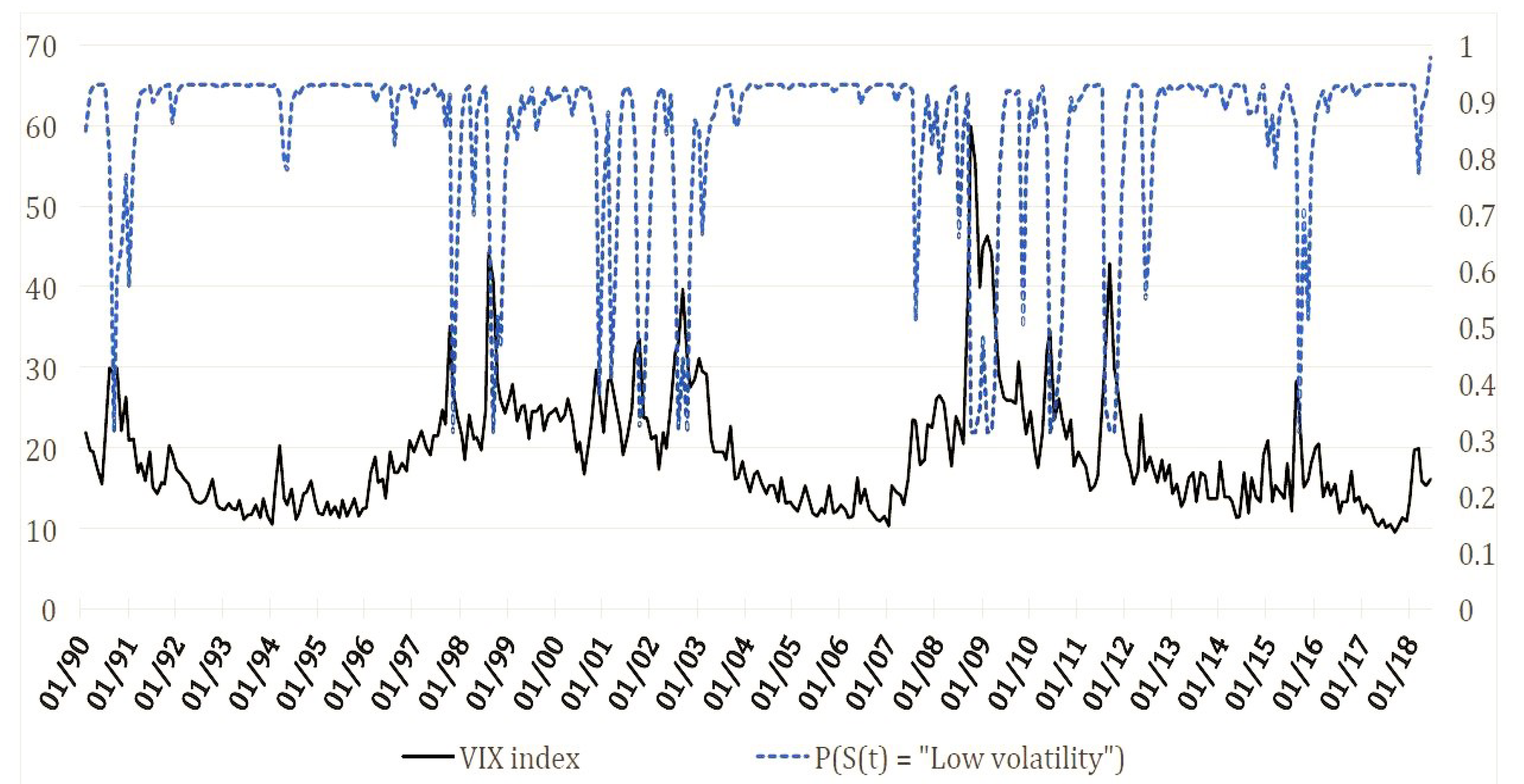
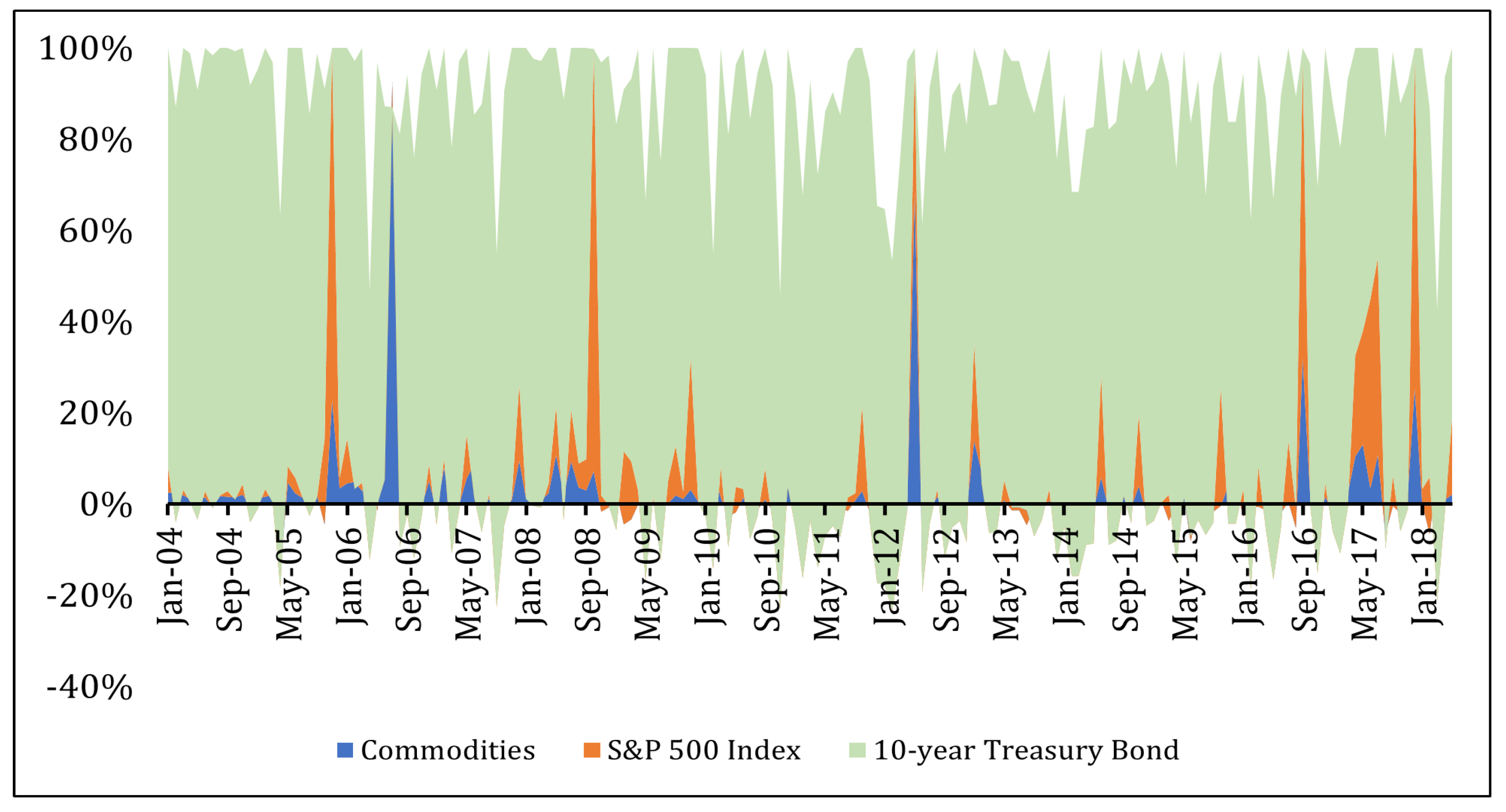
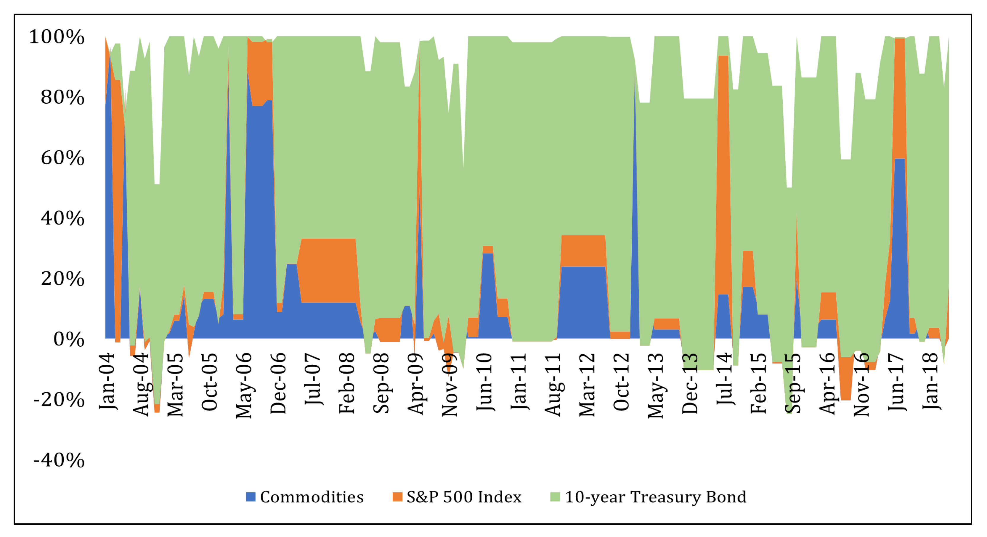
Table 1.
The tables reports mean square error forecast performances—classification by low- vs. high-risk aversion samples. The table reports the RMSFE implied by the forecasts obtained from the 12 stepwise (forward vs. backward) predictive regression models recursively implemented in our analysis. In particular, the table distinguishes between the RMSFEs obtained in periods of low vs. high market volatility (a proxy for aggregate risk aversion). Specifically, the periods of low risk aversion are identified as January 2004–December 2007 and January 2013–May 2018, while the high risk aversion sub-sample refers to January 2008–December 2012. For both the low and high risk-aversion sub-samples, we have boldfaced the forecasting model that yields the minimum RMSFE.
| Light Crude Oil | Corn | Soybeans | Wheat | Coffee | Cocoa | Sugar | Cotton No. 2 | Gold | Silver | Platinum | Orange Juice | Lumber | Live Cattle | |
|---|---|---|---|---|---|---|---|---|---|---|---|---|---|---|
| Panel A | Macro Principal Components Only | |||||||||||||
| Forward—Low | 0.0768 | 0.0748 | 0.0764 | 0.0825 | 0.0918 | 0.0703 | 0.0707 | 0.0698 | 0.0454 | 0.0801 | 0.0786 | 0.0842 | 0.0755 | 0.0758 |
| Forward—High | 0.1142 | 0.1324 | 0.1149 | 0.1264 | 0.1006 | 0.1214 | 0.1113 | 0.1125 | 0.0655 | 0.1457 | 0.1498 | 0.1043 | 0.0973 | 0.0925 |
| Backward—Low | 0.0775 | 0.0749 | 0.0762 | 0.0823 | 0.0902 | 0.0703 | 0.0709 | 0.0695 | 0.0455 | 0.0820 | 0.0785 | 0.0842 | 0.0755 | 0.0752 |
| Backward—High | 0.1166 | 0.1407 | 0.1146 | 0.1286 | 0.1023 | 0.1620 | 0.1125 | 0.1139 | 0.0726 | 0.1458 | 0.1488 | 0.1057 | 0.1130 | 0.0926 |
| Panel B | Macro Principal Components + Commodity-Specific Factors (Always Included) | |||||||||||||
| Forward—Low | 0.0823 | 0.0741 | 0.0788 | 0.0862 | 0.0990 | 0.0791 | 0.0755 | 0.0661 | 0.0493 | 0.0905 | 0.0869 | 0.0946 | 0.0813 | 0.1039 |
| Forward—High | 0.1182 | 0.1565 | 0.1140 | 0.1549 | 0.1339 | 0.1609 | 0.1180 | 0.1290 | 0.0824 | 0.1766 | 0.8282 | 0.1151 | 0.1247 | 0.1354 |
| Backward—Low | 0.0822 | 0.0736 | 0.0804 | 0.0861 | 0.1003 | 0.0798 | 0.0752 | 0.0694 | 0.0481 | 0.0912 | 0.0938 | 0.0944 | 0.0801 | 0.0984 |
| Backward—High | 0.1197 | 0.1780 | 0.1298 | 0.1666 | 0.1244 | 0.1659 | 0.1258 | 0.1414 | 0.0849 | 0.1768 | 0.7025 | 0.1270 | 0.1523 | 0.1538 |
| Panel C | Macro Principal Components + Commodity-Specific Factors | |||||||||||||
| Forward—Low | 0.0707 | 0.0725 | 0.0773 | 0.0846 | 0.0917 | 0.0728 | 0.0720 | 0.0682 | 0.0472 | 0.0829 | 0.0833 | 0.0900 | 0.0797 | 0.0833 |
| Forward—High | 0.0648 | 0.1526 | 0.1029 | 0.1468 | 0.1159 | 0.1898 | 0.1126 | 0.1214 | 0.0762 | 0.1510 | 0.1539 | 0.1086 | 0.1182 | 0.1117 |
| Backward—Low | 0.0696 | 0.0731 | 0.0780 | 0.0841 | 0.0925 | 0.0746 | 0.0717 | 0.0693 | 0.0471 | 0.0836 | 0.0840 | 0.0946 | 0.0791 | 0.0836 |
| Backward—High | 0.0634 | 0.1598 | 0.1186 | 0.1632 | 0.1248 | 0.1616 | 0.1120 | 0.1228 | 0.0825 | 0.1707 | 0.7496 | 0.1171 | 0.1448 | 0.1228 |
| Panel D | Macro Principal Components + Aggregated Commodity-Specific Factors (Always Included) | |||||||||||||
| Forward—Low | 0.0851 | 0.0775 | 0.0894 | 0.0877 | 0.0971 | 0.0750 | 0.0788 | 0.0759 | 0.0661 | 0.0836 | 0.0792 | 0.0964 | 0.0852 | 0.1154 |
| Forward—High | 0.2179 | 0.1829 | 0.1810 | 0.2229 | 0.1574 | 0.1652 | 0.2498 | 0.1851 | 0.0958 | 0.2103 | 0.2792 | 0.1316 | 0.1854 | 0.1140 |
| Backward—Low | 0.0846 | 0.0780 | 0.0786 | 0.0873 | 0.0960 | 0.0750 | 0.0793 | 0.0767 | 0.0603 | 0.0837 | 0.0792 | 0.0960 | 0.0858 | 0.0909 |
| Backward—High | 0.2113 | 0.1822 | 0.1741 | 0.2233 | 0.1614 | 0.1549 | 0.2234 | 0.2726 | 0.1169 | 0.2345 | 0.2644 | 0.1312 | 0.1884 | 0.1139 |
| Panel E | Macro Principal Components + Aggregated Commodity-Specific Factors | |||||||||||||
| Forward—Low | 0.0789 | 0.0786 | 0.0757 | 0.0852 | 0.0929 | 0.0750 | 0.0744 | 0.0724 | 0.0448 | 0.0796 | 0.0782 | 0.0959 | 0.0807 | 0.0770 |
| Forward—High | 0.1265 | 0.1593 | 0.1107 | 0.1990 | 0.1444 | 0.1374 | 0.1220 | 0.1157 | 0.0761 | 0.1428 | 0.1701 | 0.1205 | 0.1212 | 0.0969 |
| Backward—Low | 0.0795 | 0.0780 | 0.0767 | 0.0864 | 0.0909 | 0.0735 | 0.0746 | 0.0734 | 0.0458 | 0.0802 | 0.0782 | 0.0951 | 0.0850 | 0.0760 |
| Backward—High | 0.1221 | 0.1589 | 0.1395 | 0.2050 | 0.1529 | 0.1340 | 0.1521 | 0.1691 | 0.0813 | 0.1700 | 0.1750 | 0.1233 | 0.1307 | 0.0979 |
| Panel F | Macro Principal Components + Commodity-Specific Factors + Aggregated Commodity-Specific Factors (Always Included) | |||||||||||||
| Forward—Low | 0.0848 | 0.0795 | 0.0773 | 0.0945 | 0.1041 | 0.0815 | 0.0844 | 0.0746 | 0.0475 | 0.0953 | 0.0827 | 0.1038 | 0.0884 | 0.0855 |
| Forward—High | 0.2278 | 0.1739 | 0.1580 | 0.2322 | 0.1471 | 0.1722 | 0.2192 | 0.2086 | 0.1152 | 0.1963 | 0.5971 | 0.1322 | 0.1962 | 0.1467 |
| Backward—Low | 0.0862 | 0.0788 | 0.0801 | 0.0939 | 0.1064 | 0.0838 | 0.0850 | 0.0738 | 0.0481 | 0.1841 | 0.0821 | 0.1085 | 0.0882 | 0.0865 |
| Backward—High | 0.2264 | 0.1866 | 0.1607 | 0.2233 | 0.1663 | 0.1754 | 0.2242 | 0.3524 | 0.1360 | 0.2070 | 0.5627 | 0.1742 | 0.2487 | 0.1956 |
| Panel G | Benchmark AR(1) | |||||||||||||
| AR(1) | 0.0856 | 0.0867 | 0.0792 | 0.0946 | 0.0882 | 0.0799 | 0.0861 | 0.0800 | 0.0522 | 0.0955 | 0.0723 | 0.0916 | 0.0799 | 0.0463 |
Table 2.
Root mean square error forecast performances—weighting on the basis of predicted risk-aversion regime probabilities. The table reports the RMSFE implied by the forecasts obtained from the 12 stepwise (forward vs. backward) predictive regression models recursively implemented in our analysis. In particular, the table obtains the forecasts by weighting (over the entire OOS period, January 2004–May 2018) the regime-specific stepwise regression forecasts by the predicted regime probabilities obtained from a two-state HMM for the VIX index. In the different panels, we have boldfaced the forecasting model that yields the minimum RMSFE. In the first panel, we underscore the kitchen sink model (including all predictors) that delivers the lowest RMSFE when the HMM implementation is compared with the single-state one (linear predictive model).
| Light Crude Oil | Corn | Soybeans | Wheat | Coffee | Cocoa | Sugar | Cotton No.2 | Gold | Silver | Platinum | Orange Juice | Lumber | Live Cattle | |
|---|---|---|---|---|---|---|---|---|---|---|---|---|---|---|
| Panel A | HMM—Macro Principal Components Only | |||||||||||||
| 0.1014 | 0.0970 | 0.1021 | 0.1069 | 0.2446 | 0.0909 | 0.1036 | 0.0958 | 0.1088 | 0.1215 | 0.0968 | 0.1213 | 0.0857 | 0.0472 | |
| Panel B | HMM—Macro Principal Components + Commodity-Specific Factors | |||||||||||||
| 0.0871 | 0.1025 | 0.1430 | 0.1280 | 0.1153 | 0.1151 | 0.1040 | 0.0966 | 0.0989 | 0.3136 | 0.0921 | 0.1084 | 0.1074 | 0.0515 | |
| Panel C | HMM—Macro Principal Components + Aggregated Commodity-Specific Factors | |||||||||||||
| 0.1326 | 0.0976 | 0.0877 | 0.1192 | 0.1074 | 0.1258 | 0.1414 | 0.1192 | 0.0815 | 0.1142 | 0.0834 | 0.1089 | 0.0978 | 0.0526 | |
| Panel D | Stepwise Regression—Macro Principal Components Only | |||||||||||||
| Forward | 0.0830 | 0.0920 | 0.0846 | 0.0973 | 0.0925 | 0.0836 | 0.0858 | 0.0821 | 0.0516 | 0.0962 | 0.0832 | 0.0911 | 0.0824 | 0.0829 |
| Backward | 0.0817 | 0.0918 | 0.0845 | 0.0976 | 0.0916 | 0.0847 | 0.0860 | 0.0820 | 0.0531 | 0.0972 | 0.0830 | 0.0913 | 0.0843 | 0.0825 |
| Panel E | Stepwise Regression—Macro Principal Components + Commodity-Specific Factors (Always Included) | |||||||||||||
| Forward | 0.0841 | 0.0956 | 0.0838 | 0.1019 | 0.0981 | 0.0926 | 0.0880 | 0.0824 | 0.0546 | 0.1032 | 0.2508 | 0.0975 | 0.0901 | 0.0971 |
| Backward | 0.0840 | 0.0936 | 0.0867 | 0.1032 | 0.0974 | 0.0957 | 0.0887 | 0.0860 | 0.0545 | 0.1035 | 0.2128 | 0.0978 | 0.0909 | 0.0977 |
| Panel F | Stepwise Regression—Macro Principal Components + Commodity-Specific Factors | |||||||||||||
| Forward | 0.0733 | 0.0916 | 0.0824 | 0.1019 | 0.0938 | 0.0899 | 0.0862 | 0.0818 | 0.0546 | 0.0972 | 0.0853 | 0.0943 | 0.0883 | 0.0869 |
| Backward | 0.0723 | 0.0916 | 0.0849 | 0.1023 | 0.0934 | 0.0918 | 0.0862 | 0.0830 | 0.0536 | 0.0993 | 0.2267 | 0.0973 | 0.0892 | 0.0881 |
| Panel G | Stepwise Regression—Principal Components + Aggregated Commodity-Specific Factors (Always Included) | |||||||||||||
| Forward | 0.0989 | 0.0982 | 0.1038 | 0.1159 | 0.0996 | 0.0871 | 0.1144 | 0.0931 | 0.0662 | 0.1144 | 0.1080 | 0.1008 | 0.1032 | 0.1051 |
| Backward | 0.0980 | 0.0984 | 0.0971 | 0.1159 | 0.0996 | 0.0858 | 0.1100 | 0.1151 | 0.0696 | 0.1146 | 0.1041 | 0.1000 | 0.1036 | 0.0922 |
| Panel H | Stepwise Regression—Macro Principal Components + Aggregated Commodity-Specific Factors | |||||||||||||
| Forward | 0.0826 | 0.0950 | 0.0822 | 0.1131 | 0.0969 | 0.0871 | 0.0890 | 0.0824 | 0.0524 | 0.0972 | 0.0896 | 0.0994 | 0.0876 | 0.0842 |
| Backward | 0.0802 | 0.0951 | 0.0887 | 0.1162 | 0.0953 | 0.0831 | 0.0944 | 0.0874 | 0.0541 | 0.0978 | 0.0891 | 0.0986 | 0.0907 | 0.0837 |
| Panel I | Stepwise Regression—Principal Components + Commodity-Specific Factors + Aggregated Commodity-Specific Factors (Always Included) | |||||||||||||
| Forward | 0.0986 | 0.0963 | 0.0911 | 0.1185 | 0.0987 | 0.0914 | 0.1151 | 0.0945 | 0.0590 | 0.1096 | 0.1896 | 0.1037 | 0.1062 | 0.0914 |
| Backward | 0.0957 | 0.1001 | 0.0937 | 0.1193 | 0.1029 | 0.0934 | 0.1108 | 0.1347 | 0.0674 | 0.1600 | 0.1939 | 0.1116 | 0.1146 | 0.0990 |
| Panel J | Benchmark AR(1) | |||||||||||||
| AR(1) | 0.0856 | 0.0867 | 0.0792 | 0.0946 | 0.0882 | 0.0799 | 0.0861 | 0.0800 | 0.0522 | 0.0955 | 0.0723 | 0.0916 | 0.0799 | 0.0463 |
Table 3.
The table displays root mean square error forecast performances—hidden Markov chain vs. stepwise regression models. The table reports the RMSFE implied by the forecasts obtained from the three HMM and the 12 stepwise (forward vs. backward) predictive regression models recursively implemented in our analysis. In particular, the table obtains the forecasts by weighting (over the entire OOS period, January 2004–May 2018) the regime-specific stepwise regression forecasts by the predicted regime probabilities obtained from a two-state HMM for the VIX index. In the different panels we have boldfaced the forecasting model that yields the minimum RMSFE.
| Light Crude Oil | Corn | Soybeans | Wheat | Coffee | Cocoa | Sugar | Cotton No. 2 | Gold | Silver | Platinum | Orange Juice | Lumber | Live Cattle | |
|---|---|---|---|---|---|---|---|---|---|---|---|---|---|---|
| Panel A | Macro Principal Components Only | |||||||||||||
| Forward—Low | 0.0613 | 0.0592 | 0.0547 | 0.0644 | 0.0688 | 0.0555 | 0.0583 | 0.0544 | 0.0356 | 0.0638 | 0.0653 | 0.0669 | 0.0610 | 0.0625 |
| Forward—High | 0.0829 | 0.0952 | 0.0872 | 0.0932 | 0.0801 | 0.0971 | 0.0866 | 0.0842 | 0.0494 | 0.1084 | 0.0916 | 0.0874 | 0.0721 | 0.0701 |
| Backward—Low | 0.0615 | 0.0597 | 0.0545 | 0.0641 | 0.0672 | 0.0555 | 0.0584 | 0.0543 | 0.0356 | 0.0645 | 0.0655 | 0.0670 | 0.0610 | 0.0618 |
| Backward—High | 0.0817 | 0.1019 | 0.0869 | 0.0947 | 0.0826 | 0.1077 | 0.0894 | 0.0861 | 0.0517 | 0.1077 | 0.0890 | 0.0884 | 0.0847 | 0.0703 |
| Panel B | Macro Principal Components + Commodity-Specific Factors (Always Included) | |||||||||||||
| Forward—Low | 0.0644 | 0.0574 | 0.0605 | 0.0665 | 0.0791 | 0.0630 | 0.0610 | 0.0510 | 0.0378 | 0.0716 | 0.0702 | 0.0745 | 0.0659 | 0.0789 |
| Forward—High | 0.0902 | 0.1192 | 0.0866 | 0.1139 | 0.0976 | 0.1139 | 0.0918 | 0.0990 | 0.0572 | 0.1378 | 0.4112 | 0.0969 | 0.0972 | 0.0984 |
| Backward—Low | 0.0646 | 0.0570 | 0.0625 | 0.0660 | 0.0801 | 0.0642 | 0.0608 | 0.0542 | 0.0369 | 0.0723 | 0.0735 | 0.0741 | 0.0652 | 0.0736 |
| Backward—High | 0.0923 | 0.1260 | 0.0971 | 0.1267 | 0.0923 | 0.1175 | 0.0934 | 0.1059 | 0.0587 | 0.1385 | 0.3565 | 0.1059 | 0.1162 | 0.1134 |
| Panel C | Macro Principal Components + Commodity-Specific Factors | |||||||||||||
| Forward—Low | 0.0563 | 0.0579 | 0.0585 | 0.0651 | 0.0682 | 0.0575 | 0.0597 | 0.0523 | 0.0369 | 0.0658 | 0.0679 | 0.0701 | 0.0650 | 0.0671 |
| Forward—High | 0.0517 | 0.1089 | 0.0827 | 0.1080 | 0.0858 | 0.1129 | 0.0894 | 0.0905 | 0.0568 | 0.1214 | 0.0906 | 0.0893 | 0.0912 | 0.0868 |
| Backward—Low | 0.0549 | 0.0581 | 0.0593 | 0.0644 | 0.0693 | 0.0598 | 0.0594 | 0.0523 | 0.0365 | 0.0669 | 0.0675 | 0.0745 | 0.0647 | 0.0673 |
| Backward—High | 0.0507 | 0.1129 | 0.0918 | 0.1179 | 0.0930 | 0.1102 | 0.0883 | 0.0943 | 0.0586 | 0.1346 | 0.3724 | 0.0981 | 0.1083 | 0.0908 |
| Panel D | Macro Principal Components + Aggregated Commodity-Specific Factors (Always Included) | |||||||||||||
| Forward—Low | 0.0675 | 0.0630 | 0.0620 | 0.0691 | 0.0749 | 0.0596 | 0.0649 | 0.0589 | 0.0461 | 0.0665 | 0.0644 | 0.0761 | 0.0658 | 0.0908 |
| Forward—High | 0.1292 | 0.1305 | 0.1195 | 0.1373 | 0.1172 | 0.1213 | 0.1761 | 0.1295 | 0.0708 | 0.1473 | 0.1526 | 0.1013 | 0.1174 | 0.0836 |
| Backward—Low | 0.0668 | 0.0633 | 0.0585 | 0.0687 | 0.0736 | 0.0597 | 0.0651 | 0.0600 | 0.0433 | 0.0663 | 0.0645 | 0.0760 | 0.0656 | 0.0754 |
| Backward—High | 0.1216 | 0.1304 | 0.1167 | 0.1394 | 0.1195 | 0.1205 | 0.1539 | 0.1517 | 0.0747 | 0.1576 | 0.1478 | 0.1014 | 0.1187 | 0.0830 |
| Panel E | Macro Principal Components + Aggregated Commodity-Specific Factors | |||||||||||||
| Forward—Low | 0.0625 | 0.0628 | 0.0563 | 0.0661 | 0.0686 | 0.0608 | 0.0614 | 0.0568 | 0.0350 | 0.0630 | 0.0653 | 0.0749 | 0.0631 | 0.0635 |
| Forward—High | 0.0896 | 0.1122 | 0.0889 | 0.1258 | 0.1076 | 0.1047 | 0.0973 | 0.0869 | 0.0536 | 0.1128 | 0.1091 | 0.0946 | 0.0950 | 0.0713 |
| Backward—Low | 0.0631 | 0.0621 | 0.0582 | 0.0679 | 0.0676 | 0.0586 | 0.0618 | 0.0573 | 0.0359 | 0.0630 | 0.0654 | 0.0746 | 0.0661 | 0.0631 |
| Backward—High | 0.0854 | 0.1127 | 0.0962 | 0.1322 | 0.1147 | 0.1081 | 0.1132 | 0.1123 | 0.0577 | 0.1342 | 0.1163 | 0.0985 | 0.1000 | 0.0726 |
| Panel F | Macro Principal Components + Commodity-Specific Factors + Aggregated Commodity-Specific Factors (Always Included) | |||||||||||||
| Forward—Low | 0.0672 | 0.0615 | 0.0602 | 0.0734 | 0.0787 | 0.0650 | 0.0700 | 0.0588 | 0.0370 | 0.0760 | 0.0658 | 0.0829 | 0.0689 | 0.0688 |
| Forward—High | 0.1309 | 0.1352 | 0.1131 | 0.1714 | 0.1203 | 0.1244 | 0.1515 | 0.1536 | 0.0796 | 0.1532 | 0.3081 | 0.1029 | 0.1339 | 0.1055 |
| Backward—Low | 0.0678 | 0.0595 | 0.0626 | 0.0728 | 0.0815 | 0.0662 | 0.0702 | 0.0576 | 0.0377 | 0.0893 | 0.0641 | 0.0858 | 0.0690 | 0.0698 |
| Backward—High | 0.1376 | 0.1409 | 0.1157 | 0.1536 | 0.1390 | 0.1301 | 0.1587 | 0.1785 | 0.0879 | 0.1602 | 0.2736 | 0.1257 | 0.1548 | 0.1367 |
| Panel G | Benchmark AR(1) | |||||||||||||
| AR(1) | 0.0682 | 0.0676 | 0.0603 | 0.0711 | 0.0647 | 0.0635 | 0.0674 | 0.0610 | 0.0408 | 0.0748 | 0.0492 | 0.0727 | 0.0635 | 0.0356 |
Table 4.
Mean absolute error forecast performances—hidden Markov chain vs. stepwise regression models. The table reports the MAFE implied by the forecasts obtained from the three HMMs and the 12 stepwise (forward vs. backward) predictive regression models recursively implemented in our analysis. In particular, the table obtains the forecasts by weighting (over the entire OOS period, January 2004–May 2018) the regime-specific stepwise regression forecasts by the predicted regime probabilities obtained from a two-state HMM for the VIX index. In the different panels we have boldfaced the forecasting model that yields the minimum MAFE.
| Light Crude Oil | Corn | Soybeans | Wheat | Coffee | Cocoa | Sugar | Cotton No. 2 | Gold | Silver | Platinum | Orange Juice | Lumber | Live Cattle | |
|---|---|---|---|---|---|---|---|---|---|---|---|---|---|---|
| Panel A | HMM—Macro Principal Components Only | |||||||||||||
| 0.0691 | 0.0710 | 0.0673 | 0.0766 | 0.0899 | 0.0675 | 0.0786 | 0.0691 | 0.0511 | 0.0809 | 0.0588 | 0.0833 | 0.0656 | 0.0359 | |
| Panel B | HMM—Macro Principal Components + Commodity-Specific Factors | |||||||||||||
| 0.0656 | 0.0718 | 0.0757 | 0.0875 | 0.0862 | 0.0767 | 0.0781 | 0.0697 | 0.0510 | 0.1198 | 0.0611 | 0.0825 | 0.0763 | 0.0409 | |
| Panel C | HMM—Macro Principal Components + Aggregated Commodity-Specific Factors | |||||||||||||
| 0.0830 | 0.0724 | 0.0636 | 0.0861 | 0.0830 | 0.0801 | 0.0898 | 0.0783 | 0.0491 | 0.0834 | 0.0563 | 0.0877 | 0.0735 | 0.0405 | |
| Panel D | Stepwise Regression—Macro Principal Components Only | |||||||||||||
| Forward | 0.0653 | 0.0699 | 0.0628 | 0.0734 | 0.0700 | 0.0658 | 0.0678 | 0.0627 | 0.0404 | 0.0754 | 0.0672 | 0.0732 | 0.0645 | 0.0656 |
| Backward | 0.0638 | 0.0699 | 0.0626 | 0.0735 | 0.0692 | 0.0660 | 0.0684 | 0.0628 | 0.0410 | 0.0757 | 0.0671 | 0.0733 | 0.0656 | 0.0652 |
| Panel E | Stepwise Regression—Macro Principal Components + Commodity-Specific Factors (Always Included) | |||||||||||||
| Forward | 0.0662 | 0.0711 | 0.0653 | 0.0759 | 0.0773 | 0.0709 | 0.0694 | 0.0619 | 0.0417 | 0.0815 | 0.1064 | 0.0781 | 0.0704 | 0.0752 |
| Backward | 0.0664 | 0.0697 | 0.0676 | 0.0762 | 0.0765 | 0.0733 | 0.0696 | 0.0642 | 0.0413 | 0.0822 | 0.1009 | 0.0784 | 0.0716 | 0.0748 |
| Panel F | Stepwise Regression—Macro Principal Components + Commodity-Specific Factors | |||||||||||||
| Forward | 0.0585 | 0.0692 | 0.0643 | 0.0751 | 0.0705 | 0.0680 | 0.0686 | 0.0617 | 0.0421 | 0.0764 | 0.0688 | 0.0751 | 0.0693 | 0.0687 |
| Backward | 0.0571 | 0.0691 | 0.0657 | 0.0748 | 0.0705 | 0.0696 | 0.0689 | 0.0624 | 0.0416 | 0.0782 | 0.1003 | 0.0784 | 0.0701 | 0.0696 |
| Panel G | Stepwise Regression—Macro Principal Components + Aggregated Commodity-Specific Factors (Always Included) | |||||||||||||
| Forward | 0.0706 | 0.0733 | 0.0715 | 0.0793 | 0.0740 | 0.0681 | 0.0839 | 0.0685 | 0.0485 | 0.0818 | 0.0748 | 0.0791 | 0.0732 | 0.0814 |
| Backward | 0.0696 | 0.0735 | 0.0689 | 0.0792 | 0.0739 | 0.0683 | 0.0813 | 0.0729 | 0.0482 | 0.0814 | 0.0736 | 0.0787 | 0.0731 | 0.0731 |
| Panel H | Stepwise Regression—Macro Principal Components + Aggregated Commodity-Specific Factors | |||||||||||||
| Forward | 0.0650 | 0.0721 | 0.0631 | 0.0783 | 0.0716 | 0.0694 | 0.0704 | 0.0636 | 0.0404 | 0.0756 | 0.0696 | 0.0782 | 0.0681 | 0.0662 |
| Backward | 0.0642 | 0.0719 | 0.0660 | 0.0808 | 0.0706 | 0.0669 | 0.0732 | 0.0656 | 0.0417 | 0.0755 | 0.0707 | 0.0780 | 0.0701 | 0.0660 |
| Panel I | Stepwise Regression—Macro Principal Components + Commodity-Specific Factors + Aggregated Commodity-Specific Factors (Always Included) | |||||||||||||
| Forward | 0.0711 | 0.0730 | 0.0674 | 0.0857 | 0.0743 | 0.0719 | 0.0863 | 0.0697 | 0.0434 | 0.0856 | 0.0928 | 0.0824 | 0.0754 | 0.0706 |
| Backward | 0.0696 | 0.0735 | 0.0701 | 0.0833 | 0.0789 | 0.0732 | 0.0848 | 0.0732 | 0.0449 | 0.0928 | 0.0896 | 0.0860 | 0.0791 | 0.0750 |
| Panel J | Benchmark AR(1) | |||||||||||||
| AR(1) | 0.0682 | 0.0676 | 0.0603 | 0.0711 | 0.0647 | 0.0635 | 0.0674 | 0.0610 | 0.0408 | 0.0748 | 0.0492 | 0.0727 | 0.0635 | 0.0356 |
Table 5.
Root mean square error forecast performances—Markov switching vs. stepwise regression models, equally weighted. The table compares the RMSFE statistics implied by an equally-weighted average of the forecasts obtained from the three HMM and the 24 stepwise (forward and backward) predictive regression models recursively implemented in our analysis. In particular, the table obtains the forecasts by weighting (over the entire OOS period, January 2004–May 2018) the regime-specific stepwise regression forecasts by the predicted regime probabilities obtained from a two-state HMM for the VIX index. In the different panels we have boldfaced the forecasting model that yields the minimum RMSFE.
| Light Crude Oil | Corn | Soybeans | Wheat | Coffee | Cocoa | Sugar | Cotton No. 2 | Gold | Silver | Platinum | Orange Juice | Lumber | Live Cattle | |
|---|---|---|---|---|---|---|---|---|---|---|---|---|---|---|
| Panel A | HMM | |||||||||||||
| 0.0936 | 0.1039 | 0.1136 | 0.1170 | 0.1485 | 0.1036 | 0.1000 | 0.0960 | 0.0916 | 0.1754 | 0.1141 | 0.1119 | 0.0914 | 0.0673 | |
| Panel B | Stepwise Regression Models | |||||||||||||
| 0.0860 | 0.0949 | 0.0886 | 0.1086 | 0.0966 | 0.0889 | 0.0962 | 0.0920 | 0.0576 | 0.1075 | 0.1430 | 0.0986 | 0.0943 | 0.0909 | |
| Panel C | Benchmark AR(1) | |||||||||||||
| AR(1) | 0.0856 | 0.0867 | 0.0792 | 0.0946 | 0.0882 | 0.0799 | 0.0861 | 0.0800 | 0.0522 | 0.0955 | 0.0723 | 0.0916 | 0.0799 | 0.0463 |
Table 6.
Mean absolute error forecast performances—Markov switching vs. stepwise regression models, equally weighted. The table compares the MFE statistics implied by an equally-weighted average of the forecasts obtained from the three HMM and the 24 stepwise (forward and backward) predictive regression models recursively implemented in our analysis. In particular, the table obtains the forecasts by weighting (over the entire OOS period, January 2004–May 2018) the regime-specific stepwise regression forecasts by the predicted regime probabilities obtained from a two-state HMM for the VIX index. In the different panels we have boldfaced the forecasting model that yields the minimum RMSFE.
| Light Crude Oil | Corn | Soybeans | Wheat | Coffee | Cocoa | Sugar | Cotton No. 2 | Gold | Silver | Platinum | Orange Juice | Lumber | Live Cattle | |
|---|---|---|---|---|---|---|---|---|---|---|---|---|---|---|
| Panel A | HMM | |||||||||||||
| 0.7530 | 0.0669 | 0.0646 | 0.0834 | 0.0801 | 0.0774 | 0.0762 | 0.0672 | 0.0488 | 0.0891 | 0.0606 | 0.0787 | 0.0718 | 0.0391 | |
| Panel B | Stepwise Regression Models | |||||||||||||
| 0.0656 | 0.0713 | 0.0663 | 0.0780 | 0.0731 | 0.0693 | 0.0744 | 0.0658 | 0.0429 | 0.0802 | 0.0818 | 0.0782 | 0.0709 | 0.0709 | |
| Panel C | Benchmark AR(1) | |||||||||||||
| AR(1) | 0.0682 | 0.0676 | 0.0603 | 0.0711 | 0.0647 | 0.0635 | 0.0674 | 0.0610 | 0.0408 | 0.0748 | 0.0492 | 0.0727 | 0.0635 | 0.0356 |
Table 7.
Realized portfolio performance of mean-variance strategies based on HMM vs. stepwise regression forecasts (no transaction costs). The table reports a range of realized OOS performance measures obtained from recursive mean-variance portfolio optimization strategies over a January 2004–May 2018 sample. The 16 models reported are obtained as three HMMs with regimes plus the best 12 stepwise predictive regressions selected on the basis of their RMSFE, and the AR(1) benchmark. We boldface the highest realized performances.
| = 0.1 | = 0.25 | = 0.5 | ||||||||||
| Mean Return | Std. Dev. | Sharpe Ratio | Realized MV | Mean Return | Std. Dev. | Sharpe Ratio | Realized MV | Mean Return | Std. Dev. | Sharpe Ratio | Realized MV | |
| HMM Macro Factors | 0.0006 | 0.0198 | 0.0962 | 0.0005 | 0.0001 | 0.0190 | 0.0258 | 0.0001 | 0.0002 | 0.0182 | 0.0328 | 0.0001 |
| HMM Macro and Commodity-Specific Factors | 0.0020 | 0.0388 | 0.1813 | 0.0020 | −0.0002 | 0.0351 | −0.0246 | −0.0004 | 0.0019 | 0.0268 | 0.2446 | 0.0017 |
| HMM Macro and Aggregate Commodity Factors | 0.0026 | 0.0429 | 0.2095 | 0.0025 | 0.0020 | 0.0185 | 0.3660 | 0.0019 | 0.0012 | 0.0213 | 0.1977 | 0.0011 |
| Stepwise PCs—Forward | 0.0001 | 0.0181 | 0.0035 | 0.0001 | −0.0001 | 0.0183 | −0.0109 | −0.0001 | 0.0002 | 0.0166 | 0.0318 | 0.0001 |
| Stepwise PCs—Backward | −0.0003 | 0.0220 | −0.0409 | −0.0003 | −0.0002 | 0.0202 | −0.0339 | −0.0002 | 0.0002 | 0.0182 | 0.0291 | 0.0001 |
| Stepwise PCs and Commodity-Specific Factors (always incl.)—Forward | 0.0032 | 0.0376 | 0.2932 | 0.0031 | 0.0032 | 0.0369 | 0.3000 | 0.0030 | 0.0037 | 0.0361 | 0.3548 | 0.0034 |
| Stepwise PCs and Commodity-Specific Factors (always incl.)—Backward | −0.0025 | 0.0388 | −0.2229 | −0.0026 | −0.0024 | 0.0379 | −0.2198 | −0.0026 | −0.0027 | 0.0381 | −0.2442 | −0.0030 |
| Stepwise PCs and Commodity-Specific Factors—Forward | −0.0021 | 0.0291 | −0.2505 | −0.0021 | −0.0005 | 0.0312 | −0.0527 | −0.0006 | 0.0011 | 0.0246 | 0.1578 | 0.0010 |
| Stepwise PCs and Commodity-Specific Factors—Backward | −0.0016 | 0.0274 | −0.1975 | −0.0016 | −0.0016 | 0.0271 | −0.1988 | −0.0016 | −0.0017 | 0.0253 | −0.2266 | −0.0018 |
| Stepwise PCs and Aggregate Commodity Factors (always incl.)—Forward | −0.0030 | 0.0334 | −0.3088 | −0.0030 | −0.0024 | 0.0322 | −0.2582 | −0.0025 | −0.0024 | 0.0322 | −0.2577 | −0.0026 |
| Stepwise PCs and Aggregate Commodity Factors (always incl.)—Backward | −0.0020 | 0.0329 | −0.2129 | −0.0021 | −0.0020 | 0.0361 | −0.1890 | −0.0021 | −0.0007 | 0.0322 | −0.0796 | −0.0010 |
| Stepwise PCs and Aggregate Commodity Factors—Forward | −0.0010 | 0.0179 | −0.2020 | −0.0011 | −0.0007 | 0.0184 | −0.1408 | −0.0008 | −0.0008 | 0.0183 | −0.1520 | −0.0009 |
| Stepwise PCs and Aggregate Commodity Factors—Backward | 0.0002 | 0.0319 | 0.0259 | 0.0002 | 0.0002 | 0.0319 | 0.0203 | 0.0001 | −0.0005 | 0.0320 | −0.0594 | −0.0008 |
| Stepwise PCs and Aggregate Commodity- Specific Factors (always incl.)—Forward | 0.0019 | 0.0427 | 0.1550 | 0.0018 | 0.0005 | 0.0417 | 0.0400 | 0.0003 | 0.0011 | 0.0337 | 0.1151 | 0.0008 |
| Stepwise PCs and Aggregate Commodity- Specific Factors (always incl.)—Backward | −0.0073 | 0.1213 | −0.2095 | −0.0081 | 0.0026 | 0.0370 | 0.2408 | 0.0024 | 0.0009 | 0.0341 | 0.0881 | 0.0006 |
| AR(1) Benchmark | −0.0001 | 0.0154 | −0.0296 | −0.0001 | −0.0001 | 0.0154 | −0.0298 | −0.0002 | −0.0001 | 0.0154 | −0.0302 | −0.0002 |
Table 8.
Realized portfolio performance of mean-variance strategies based on HMM vs. stepwise regression forecasts (with transaction costs). The table reports the realized OOS performance measures obtained from recursive mean-variance portfolio optimization strategies over a January 2004–May 2018 sample. The 16 models reported are obtained as three HMMs with regimes plus the best 12 stepwise predictive regressions selected on the basis of their RMSFE, and the AR(1) benchmark. Transaction costs are not only imputed ex post as a function of the portfolio trades executed, but also ex ante in the sense that only monthly portfolio changes that are expected ex ante to increase mean-variance utility in excess of the loss caused by the transaction costs are executed. We boldface the highest realized performances.
| = 0.1 | = 0.25 | = 0.5 | ||||||||||
| Mean Return | Std. Dev. | Sharpe Ratio | Realized MV | Mean Return | Std. Dev. | Sharpe Ratio | Realized MV | Mean Return | Std. Dev. | Sharpe Ratio | Realized MV | |
| HMM Macro Factors | 0.0002 | 0.0193 | 0.0330 | 0.0002 | −0.0020 | 0.0218 | −0.3101 | −0.0020 | −0.0016 | 0.0214 | −0.2637 | −0.0017 |
| HMM Macro and Commodity-Specific Factors | 0.0029 | 0.0333 | 0.3007 | 0.0028 | 0.0011 | 0.0211 | 0.1764 | 0.0010 | 0.0012 | 0.0213 | 0.1977 | 0.0012 |
| HMM Macro and Aggregate Commodity Factors | 0.0024 | 0.0473 | 0.1727 | 0.0022 | 0.0027 | 0.0277 | 0.3362 | 0.0026 | 0.0021 | 0.0194 | 0.3697 | 0.0020 |
| Stepwise PCs—Forward | 0.0027 | 0.0306 | 0.3008 | 0.0026 | 0.0022 | 0.0306 | 0.2445 | 0.0020 | 0.0021 | 0.0304 | 0.2447 | 0.0019 |
| Stepwise PCs—Backward | 0.0026 | 0.0363 | 0.2506 | 0.0026 | 0.0025 | 0.0360 | 0.2388 | 0.0023 | 0.0029 | 0.0346 | 0.2923 | 0.0026 |
| Stepwise PCs and Commodity-Specific Factors (always incl.)—Forward | 0.0022 | 0.0541 | 0.1378 | 0.0020 | 0.0030 | 0.0530 | 0.1942 | 0.0026 | 0.0015 | 0.0506 | 0.1035 | 0.0009 |
| Stepwise PCs and Commodity-Specific Factors (always incl.)—Backward | −0.0015 | 0.0352 | −0.1495 | −0.0016 | −0.0010 | 0.0341 | −0.1051 | −0.0012 | −0.0004 | 0.0347 | −0.0373 | −0.0007 |
| Stepwise PCs and Commodity-Specific Factors—Forward | 0.0011 | 0.0089 | 0.4356 | 0.0011 | 0.0010 | 0.0082 | 0.4170 | 0.0010 | 0.0010 | 0.0083 | 0.4304 | 0.0010 |
| Stepwise PCs and Commodity-Specific Factors—Backward | 0.0017 | 0.0248 | 0.2440 | 0.0017 | 0.0029 | 0.0214 | 0.4731 | 0.0029 | 0.0011 | 0.0217 | 0.1726 | 0.0010 |
| Stepwise PCs and Aggregate Commodity Factors (always incl.)—Forward | 0.0013 | 0.0213 | 0.2140 | 0.0013 | 0.0009 | 0.0240 | 0.1344 | 0.0009 | 0.0009 | 0.0240 | 0.1266 | 0.0007 |
| Stepwise PCs and Aggregate Commodity Factors (always incl.)—Backward | −0.0003 | 0.0219 | −0.0431 | −0.0003 | −0.0003 | 0.0218 | −0.0408 | −0.0003 | 0.0002 | 0.0238 | 0.0262 | 0.0000 |
| Stepwise PCs and Aggregate Commodity Factors—Forward | 0.0011 | 0.0198 | 0.1996 | 0.0011 | 0.0010 | 0.0194 | 0.1774 | 0.0009 | 0.0008 | 0.0169 | 0.1577 | 0.0007 |
| Stepwise PCs and Aggregate Commodity Factors—Backward | −0.0023 | 0.0447 | −0.1746 | −0.0024 | −0.0022 | 0.0446 | −0.1690 | −0.0024 | 0.0012 | 0.0164 | 0.2497 | 0.0011 |
| Stepwise PCs and Aggregate Commodity- Specific Factors (always incl.)—Forward | 0.0066 | 0.0410 | 0.5590 | 0.0065 | 0.0065 | 0.0337 | 0.6651 | 0.0063 | 0.0063 | 0.0338 | 0.6452 | 0.0060 |
| Stepwise PCs and Aggregate Commodity- Specific Factors (always incl.)—Backward | 0.0066 | 0.0410 | 0.5590 | 0.0065 | 0.0065 | 0.0337 | 0.6651 | 0.0063 | 0.0073 | 0.0325 | 0.7738 | 0.0070 |
| AR(1) Benchmark | 0.0011 | 0.0133 | 0.2958 | 0.0011 | 0.0011 | 0.0133 | 0.2962 | 0.0011 | 0.0011 | 0.0132 | 0.2975 | 0.0011 |
Publisher’s Note: MDPI stays neutral with regard to jurisdictional claims in published maps and institutional affiliations. |
© 2022 by the authors. Licensee MDPI, Basel, Switzerland. This article is an open access article distributed under the terms and conditions of the Creative Commons Attribution (CC BY) license (https://creativecommons.org/licenses/by/4.0/).
Share and Cite
MDPI and ACS Style
Guidolin, M.; Pedio, M. Switching Coefficients or Automatic Variable Selection: An Application in Forecasting Commodity Returns. Forecasting 2022, 4, 275-306. https://0-doi-org.brum.beds.ac.uk/10.3390/forecast4010016
AMA Style
Guidolin M, Pedio M. Switching Coefficients or Automatic Variable Selection: An Application in Forecasting Commodity Returns. Forecasting. 2022; 4(1):275-306. https://0-doi-org.brum.beds.ac.uk/10.3390/forecast4010016
Chicago/Turabian StyleGuidolin, Massimo, and Manuela Pedio. 2022. "Switching Coefficients or Automatic Variable Selection: An Application in Forecasting Commodity Returns" Forecasting 4, no. 1: 275-306. https://0-doi-org.brum.beds.ac.uk/10.3390/forecast4010016